Journal of Health Economics 19 2000 983–1006
www.elsevier.nlrlocatereconbase
Efficiency and administrative costs in
primary care
Antonio Giuffrida, Hugh Gravelle
), Matthew Sutton
National Primary Care Research and DeÕelopment Centre, Centre for Health Economics, UniÕersity of York, York, YO10 5DD, UK
Received 8 July 1999; received in revised form 14 March 2000; accepted 10 May 2000
Abstract
We use a formal model to examine the implications of endogenous managerial effort for the interpretation and estimation of efficiency in health care organisations. The model is applied to investigate the doubling of the cost of administering primary care in England in real terms between 1989r1990 and 1994r1995. The main cost determinant was the number
Ž .
of general practitioners GPs , and there were economies of scale but not of scope. Fundholding had a positive but small effect on administrative costs, so that the recent abolition of fundholding may do little to reduce primary care administrative costs. After allowing for changes in the numbers of primary care practitioners, the quality of primary care and the extent of fundholding, most of the increase in costs was unexplained, and may reflect additional but unmeasured increases in the administrative burden associated with the 1990 reforms. There was little variation in relative efficiency across areas.q2000 Elsevier Science B.V. All rights reserved.
JEL classification: I18; I11; L31
Keywords: Primary care; Administrative costs; Efficiency measurement; Performance indicators; Cost
function
)Corresponding author. Tel.:q44-1904-433663; fax:q44-1904-432700.
Ž .
E-mail address: [email protected] H. Gravelle .
0167-6296r00r$ - see front matterq2000 Elsevier Science B.V. All rights reserved.
Ž .
1. Introduction
This paper estimates a cost function for primary care administration using a
Ž .
panel of data for Family Health Service Authorities FHSAs in England. It makes a number of methodological and substantive contributions.
First, we set out a simple model of managerial effort and administrative costs. We use the model to examine the welfare implications of endogenous managerial effort and the estimation of efficiency in health care by standard econometric
Ž .
methods Schmidt and Sickles, 1984 . The paper complements and extends the debate in the Symposium on Frontier Estimation in the Journal of Health
Economics1 which focused on alternative methods for estimating efficiency, rather
than on the welfare interpretation of the estimates.
Second, we examine how far the doubling of administrative expenditure between 1989r1990 and 1994r1995 is due to shifts in the cost function and changes in administrative tasks. One of the justifications for the current sweeping changes in the organisation of the National Health Service is that the introduction
Ž .
of the internal market and changes to the general practitioner GP contract from 1990r1991 onward led, amongst other things, to an increase in administration
Ž .
costs Department of Health, 1997 . By estimating an administrative cost function for primary care services we provide some evidence of the possible effect of the internal market, in particular of the spread of fundholding practices, on administra-tive costs in primary care.
Third, the cost function enables us to examine the extent of economies of scale and scope in primary care administration. The recent reorganisation of the NHS has led to a devolution of some administrative responsibilities for primary care
Ž .
from health authorities to more numerous lower level units Primary Care Groups .
Ž
It also expected that the reforms will lead health authorities to merge Department
.
of Health, 1997 .
Fourth, the estimated cost function is relevant for the current policy focus on explicit measurement of performance and initiatives to reduce administrative cost
ŽDepartment of Health, 1997; NHS Executive, 1998 . We use the estimated cost.
function to examine differences in administrative expenditure across health author-ities and the potential gains achievable if such differences can be attributed to differences in efficiency.
Section 2 outlines the institutional background, presents a simple model of the determinants of administrative costs, and discusses whether differences in costs imply differences in efficiency. Section 3 describes the data, regression model and estimation methods. Section 4 presents and discusses the results. Section 5 concludes.
1
A. Giuffrida et al.rJournal of Health Economics 19 2000 983–1006 985 2. Modelling inefficiency
In this section we set out a simple model of the determinants of administrative costs. Although the setting is English primary care, our modelling of efficiency is relevant for other health care systems. We suppose that endogenous managerial effort affects administrative cost, so that what is usually measured as exogenous inefficiency is endogenous. This has implications both for the welfare interpreta-tion of the empirical results and for the estimainterpreta-tion of the administrative cost
Ž .
function. Our approach is similar to Gaynor and Pauly 1990 but in a different institutional setting with different property rights.
2.1. Institutional background
Ž 2.
During the period of our analysis 1989r1990 to 1994r1995 primary care in England was administrated by 90 FHSAs covering geographically defined popula-tions of about 500,000.3 FHSAs were independent public bodies, receiving their funding direct from the Department of Health.
Prior to April 1990 FHSAs were mainly responsible for administering payments to general practitioners, practice nurses, dentists, opticians, and pharmacies provid-ing primary care services. The reforms of 1990 expanded the tasks of FHSAs and seem to have imposed an increasing administrative burden. The new GP contract increased the range of activities for which GPs could claim payment from the FHSA. FHSAs had an increased monitoring role and responsibility for improving the quality of primary care by feeding back information to GPs and encouraging peer review via Medical Audit Advisory Groups, which was compulsory for
Ž .
practices after 1992 Fry, 1993 . From April 1991 practices were permitted to hold budgets to spend on certain types of secondary care and on pharmaceuticals. In the first year the budgets were set by Regional level managers, though some burden would have fallen on the FHSAs as well. After the first year, FHSAs had to negotiate the budget for fundholders, to hold the funds and make payments for services purchased when directed by the fundholders, to monitor financial out-comes and to check on the use to which fundholders put any budget surplus
ŽLevitt et al., 1995 . The reforms would be expected to lead to a growth in the.
administrative tasks.
2
These are financial years running from April 1 to March 31.
3
2.2. AdministratiÕe technology
The FHSA manager controls a vector of administrative inputs L , . . . , L1 n
Žclerks, office space, computers, etc. with parametric input prices w , . . . ,w . The. 1 n
Ž .
manager receives a salary w . Defining L0 s L , . . . , L1 n total administrative expenditure is w0qwL. The authority’s main task is administering payments to
Ž
primary care practitioners and service providers GPs, dentists, opticians,
pharma-.
cies .
There is an administrative technology defined by4
g a, q, L; x
Ž
.
G0, ga)0, gq-0, gL-0, gx-0Ž .
1where a is the effort of the manager, q is a vector of endogenous variables which can be influenced by health authority managers, and x is a vector of exogenous variables.
We think of q as measuring some aspects of the quality of care provided in the authority, for example the proportion of women aged 25–64 who receive a cervical smear. Managers can increase the proportion by providing information and advice to general practitioners. Increases in the proportion can trigger addi-tional payments to GPs and hence addiaddi-tional processing by the FSHA, so that an increase in q may be costly.
Ž .
The components of x include population characteristics such as morbidity and characteristics of the authority, such as its area and transport facilities. We
Ž
assume that the numbers of primary care professionals GPs, dentists, opticians,
. 5
etc. to be serviced by the authority are also exogenous and that the more professionals, the greater the administrative services required in connection with payments, budget setting and monitoring. We also assume that the number of fundholding GPs is exogenous as far as the managers of FHSAs are concerned.
The distinction between the exogenous x and endogenous q is important for the modelling of managerial decision making and for the interpretation of the regression results. However, our particular assumptions about whether quality and the numbers of fundholding GPs are endogenous or exogenous are illustrative, not essential. We test for the endogeneity of our quality measure and for the numbers of fundholding GPs in the empirical section.
2.3. Managerial preferences
Managers are assumed to act as if they had quasi-altruistic preferences. They like income and dislike effort, but also are concerned about the net benefits
4 Ž .
g , g , g are vectors of partial derivatives with respect to the components of q, L, y. We defineq L x
the components of x so that increases in x tighten the technology constraint and assume that the technology is smooth enough to yield a cost function with continuous second derivatives.
5
Contracts with professionals were nationally negotiated and the entry of GPs into areas was
Ž .
A. Giuffrida et al.rJournal of Health Economics 19 2000 983–1006 987
produced by their health authority and about the costs of administering it. They are similar to the quasi-altruistic providers and hospital managers of other health
Ž .
service models Ellis, 1998; Halonen and Propper, 1999 and contrast with the
Ž
selfish bureaucrats of classical bureaucracy models Niskanen, 1971; Wintrobe
.
1997 . Quasi altruism may arise because the health service attracts managers with such preferences. Alternatively it may be due to managers’ more selfish concerns about career prospects or professional reputation for good management. Whilst managers do not compete directly with each other, the large number of authorities operating in similar circumstances provides a benchmark against which they can be judged. Managers may therefore feel that they will be judged in part on their ability toArun a tight shipB.
The managerial utility function is
msm a, q, L; x ,w
Ž
.
sb b q ; xŽ
.
yb wLyb a2qb wŽ .
20 1 2 3 0
Ž .
where bi)0, is0, . . . ,3. b q; x is the net social benefit from the health care provided with given numbers of primary care professional supplying primary care services of quality q to a given population. Note that b is net of the costs of GPs and other professionals, pharmaceuticals prescribed etc.
Managers’ concerns about administrative costs are captured in b1. Professional pride or greater altruism tends to increase b1. Conversely managers who feel that their prestige and status are increased if they have more subordinates will tend to have smaller b1.
If we define a as effective effort, the parameterb2 can capture the tastes and the productivity of the manager. For example, suppose that managers care about the number of hours they work and that h hours input by a manager of calibre w
yields effective effort ashw. Then bXh2 is the cost of h hours and b a2s
2 2
Ž X 2 . 2
b2rw a is the cost of effective effort where b2 reflects both the manager’s
Ž X
. Ž .
preferences b2 and productivity w .
2.4. Managerial effort and administratiÕe costs
We examine the decisions by the manager in three stages.6At stage 1, for given
a, q, x, and w, the manager chooses L subject to the technological constraint
Ž .
g a, q, L; x G0. Even if managerial salary w0 is an increasing function of
administrative expenditure we assume that the manager’s preference parameters and the relationship between salary and administrative expenditures are such that, for given a, q, x, and w, managerial utility is a monotonically decreasing function
6
We assume that b is concave in q and that the feasible set defined by the administrative
Ž .
of administrative expenditure.7 Hence, the manager’s decision is equivalent to choosing L to minimise the cost of the non-managerial inputs. The preference parameters b have no effect on the stage 1 decision: they merely scale the input
Ž .
prices. The optimal input vector L a, q; x,w gives the administrative cost function for given effort:
Csw0qwL a, q ; x ,w
Ž
.
sC a, q ; x ,w ,Ž
.
Ca-0,Cq)0,Cx)0,CwsL3
Ž .
The stage 2 decision is to choose managerial effort, for given q, to maximise
msb0b q ; x
Ž
.
yb1C a, q ; x ,wŽ
.
yb2a2qŽ
b3qb1.
w0Ž .
4The first order condition is
yb1Ca
Ž
a, q ; x ,w.
y2b2as0Ž .
50 0Ž .
yielding the optimal effort decision a sa q; x,w,b and the administrative cost function
C0sC a
Ž
0Ž
y ; x ,w,b.
, q ; x ,w.
sC0Ž
q ; x ,w,b.
Ž .
6The comparative static properties are straightforward. Effort is increasing inb1
and decreasing in b2. Increases in quality q and the exogenous Õariables x
(
increase effort if and only if they increase the productiÕity of effort Ca q-0,
)
Ca x-0 .
Unsurprisingly, managers supply more effort, at given q, if they place greater weight on the administration cost relative to their effort cost. More productive managers, who have smaller marginal costs of effective effort, also supply a greater amount of effective effort, though they may put in fewer nominal hours. Although increases in q or x increase administration costs, their effect on effort depends on whether they increase the cost-reducing effects of additional effort. Alternatively, since Ca qsCq aand Ca xsC , effort increases with these variablesx a
if it reduces their marginal cost.
The stage three decision is to choose quality, taking account of its effect on the net benefits b and on administrative costs C0. The first order condition is,
remembering that a0 is chosen optimally,
b b yb C y
Ž
b C q2b a0.
a0sb bŽ
q, x.
yb CŽ
a0, q ; x ,w.
s0 0 q 1 q 1 a 2 q 0 q 1 q7
Ž .
7
A. Giuffrida et al.rJournal of Health Economics 19 2000 983–1006 989
00 00Ž . 00 0Ž 00 . 00Ž .
The optimal q sq x,w,b and a sa q ; x,w,b sa x,w,b give the observed level of administrative costs in the authority:
CsC a
Ž
00Ž
x ,w,b.
, q00Ž
x ,w,b.
; y, p, k ,w.
sC00Ž
x ,w,b.
Ž .
8Ž . Ž .
Using the first order conditions 7 and 5 we see that quality is increasing in
b0 but that the effects of the other preference parameters depends on Ca q because they will also induce changes in effort and therefore in the marginal cost of quality. Thus
00
Eq 0
sgnEb ssgn yCqyb1C aq a b2
Ž .
91 00
Eq 0
sgnEb ssgn yb1C aq a b2
Ž
10.
2
Since a0 )0 and a0 -0 we see that if additional effort reduces the marginal
b1 b2
cost of quality, then quality decreases with b2 but may increase or fall with b1.
Increases in the effort parameterb2 reduce effort and this increases the marginal cost of quality, thereby reducing its optimal level. However, although increases in
b1 increase the value of cost reductions, increase effort and reduce the marginal cost of quality, this effect is counteracted by the fact that increases in quality are costly and a greater weight is attached to such increases.
2.5. Policy implications
In Section 3 we estimate an administrative cost function from data on adminis-trative expenditure and its determinants. If their preference parameters differ, managers will supply different amounts of effort, conditional on the other determi-nants of administrative expenditure. Those with lower effort levels will have higher administrative costs. What is the policy significance of such cost differ-ences?
Suppose that the welfare function is
Ssg b q ; x
Ž
.
yg wLyg a2Ž
11.
0 1 2
Welfare is identical to the manager’s objective function except for the possibly different weights on the net benefits, the costs of the non-managerial administra-tive inputs and the manager’s effort costs. Assume that input prices w measure the social opportunity costs of the inputs and that the social cost of managerial effort isg2a2. The salary of the manager is a transfer payment.
Without loss of generality, we can setg2sb2,8 so that the welfare function takes full account of the manager’s private effort cost. Although distributional concerns about the relative merits of patients, providers, taxpayers and administra-tors are important in health care, they are picked up in the weights on net benefits and administrative costs.
It seems plausible that g1)b1)0. We assume that on balance managers prefer smaller administrative expenditure but that they do not fully internalise the social effects of increased administrative expenditure.
It is also plausible that g0)b0)0, so that managers are semi-altruistic as regards the social benefits and costs of the health care outputs produced in their authority. However, the weight they place on them relative to their effort costs may be smaller than the social weight.
Welfare is maximised in three stages. At stage 1, expenditure on the administra-tive inputs L is minimised for given levels of managerial effort and q. Since the manager’s utility is decreasing in administrative cost, the manager chooses the socially optimal mix of administrative inputs for a given level of managerial effort and quality. The welfare function can be therefore be written as
SsS a, q ; x ,w
Ž
.
sg byg wLyg a20 1 2
sg0b q ; x
Ž
.
yg1C a, q ; x ,wŽ
.
yg2a2qg1w0Ž
12.
Since the welfare function differs from the managerial utility function only in
) 0Ž .
the weights, the socially optimal stage 2 effort is a sa q; x,w,g and the
)) 00Ž .
socially optimal stage 3 decision on quality is q sq x,w,g . The maximised social welfare is
S))sS a
Ž
)), q)); x ,w.
2
)) )) )) ))
sg0b q
Ž
, x.
yg1C aŽ
, q ; x ,w.
yg2Ž
a.
qg1w0sS))
Ž
x ,w,g.
Ž
13.
)) 00Ž . 0Ž )) .
where a sa x,w,g sa q ; x,w,g .
0Ž . Ž 0Ž . .
The cost function C q; x,w,g sC a q; x,w,g , q; x,w,g shows the adminis-trative costs for given quality when the adminisadminis-trative inputs and managerial effort
0Ž .
are chosen to maximise welfare. Call C q; x,w,g the first best cost function and
0Ž .
suppose for the moment that C q; x,w,g is known. Given the assumptions about
8
With more than one health authority we must allow for the fact that there will possibly be different
Ž i i i i.
vectors b0,b1,b2,b3 of managerial preference parameters across the health authorities. There is no reason why the social preference parameter on administration costs should differ across authorities. It could be argued that the parameter on net benefits could vary with the area to reflect say greater value being placed on benefits accruing in poorer areas. There seem to be no such distributional considera-tions which would suggest that managerial preferences as regards the cost of effort should be respected in some areas but not in others. Hence, we would havegi possibly varying across areas,gisg,;i
0 1 1
andgisbi,;i.
A. Giuffrida et al.rJournal of Health Economics 19 2000 983–1006 991
managerial and social preference weights, it is obvious from the first order
Ž . 9
condition on effort choice 5 that the manager chooses too little effort. Conse-quently the authority will lie above the first best frontier:
C0
Ž
q ; x ,w,b.
yC0Ž
q ; x ,w,g.
)0Ž
14.
However, comparison of the welfare and managerial utility maximising deci-sions shows that some care is required in drawing welfare implications from the fact that an authority lies above the first best cost frontier. The welfare loss
S a
Ž
)), q)); x ,w.
yS aŽ
00, q00; x ,w.
sS a
Ž
00Ž
x ,w,g.
, q00Ž
x ,w,g.
; x ,w.
yS a
Ž
00Ž
x ,w,b.
, q00Ž
x ,w,b.
; x ,w.
Ž
15.
arises because the manager is incompletely altruistic: she chooses the wrong effort
Ž .
and endogenous quality. The excess administrative expenditure 14 fails to reflect the welfare loss for two reasons. First, it does not allow for the fact that quality as well as effort diverge from the social optimum cost. If q is in fact endogenous in the sense that it is under the control of the manager, we have to take account of the
Ž . Ž .
first type of error in using 14 as a measure of 15 .
Second, even if quality is exogenous, so that only managerial effort is at issue,
Ž . 0Ž .
14 ignores the cost of the manager’s effort. Since a q; x,w,g minimises
Ž . 2 10
C a, q; x,w qg2arg1 the welfare loss at given quality is proportional to
2
0 0 0
C
Ž
q ; x ,w,b.
yCŽ
q ; x ,w,g.
qŽ
g2rg1.
aŽ
q ; x ,w,b.
2
0 0 0
ya
Ž
q ; x ,w,g.
- CŽ
q ; x ,w,b.
yCŽ
q ; x ,w,g.
Ž
16.
The importance of the over-estimation of the welfare loss depends on the relative magnitudes of the difference between managerial effort costs at the private and social optimum and the difference between administrative costs at these
Ž
points. It is plausible that the difference between the true welfare loss the left
Ž .. Ž
hand side of 16 and the measured difference in administrative costs the right
.
hand side is not large. Managerial effort cost is likely to be negligible compared with the cost of the other administrative inputs, so that the difference between the cost of privately and socially optimal managerial effort is also negligible and so
9The effect of the preference parameter on effort isEa0rEb syC rŽbC qb .)0 and we 1 a 1 a a 2
have assumed thatb1-g1.
10
Although the manager’s salary cost w0 is not a social cost of producing administrative services
Žthe social cost of managerial effort isg a2.and is included in Csw qwL, it drops out of the
2 0
0Ž . 0Ž .
Ž .
the difference in administrative costs in 14 may be a reasonable measure of the welfare loss from the manager’s suboptimal effort.
The administrative cost function which can be estimated is not the first best
0Ž .
cost function C q; x,w,g but the function corresponding to the effort level of the
0Ž max. max
area with the greatest effort level: C q; x,w,b where b is the preference vector of the area with the greatest weight on administrative cost. Sincebmax-g , 1 1 0Ž i i i i.
comparison of the administration cost C q ; x ,w ,b in area i with the
esti-0Ž i i i max.
mated function C q ; x ,w ,b will underestimate the administrative cost reduction which could be achieved by supplying the first best amount of effort.
Even in these circumstance there is value in estimating the cost function. The differences in costs between areas can be used to identify those where there is apparently poor performance which merits further more detailed investigation. The differences in costs which remain after such investigation provide some guidance as the potential welfare gains from introducing incentive schemes and other mechanisms for improving performance.
2.6. Implications for estimation results
The second reason for introducing a simple formal model of managerial decisions is to guide the estimation of the cost function and the interpretation of the results. Assume for the moment that managerial effort is the only endogenous variable in the cost function. Effort will be a function of all the other variables in the cost function and managerial preferences. To illustrate the implications, suppose that, after suitable transformation, the true cost function in area i at time t is
ci tsd0qd1x1 i tqd2x2 i tqd3ai tq´i t
Ž
17.
Ž .
where c is the transformed administrative cost, xi t 1 i t is an observable exogenous variable and x2 i t is also exogenous but unobserved. ´i t is a zero mean i.i.d. error term reflecting unobservable exogenous factors which do not influence managerial effort and are uncorrelated with the x1 i t, x2 i t. Assume that the unobserved variable is correlated with the observed:
x2 i tsf0qf0 iqf1x1 i tqri t
Ž
18.
and r a zero mean i.i.d. error. Endogenous managerial effort isi t
ai tsa0qa0 iqa1x1 i tqa2x2 i tqÕi t
Ž
19.
where a reflects authority specific factors and Õ is a zero mean i.i.d. error
0 i i t
term.
A. Giuffrida et al.rJournal of Health Economics 19 2000 983–1006 993
should be used. Random effects estimation requires that the area effects are not
Ž .
correlated with x1 i t Baltagi, 1995 . But the omitted x2 i t are correlated with x1 i t
by assumption and the omitted managerial effort variable is correlated with x1 i t
Ždirectly and indirectly via x2 i t. from the manager’s optimisation problem. Thus
the endogeneity of managerial effort indicates that we should use fixed effects procedures to estimate the cost function.
The coefficients in the estimated cost equation
ci tsd0q
Ý
d D0 j jqd x1 1 i tŽ
20.
js2
where the D are area dummies, satisfyj
plim d0sd0q
Ž
d2qd a3 2.
f0Ž
21.
plim d0 is
Ž
d2qd a3 2.
f0 iqd a3 0 iŽ
22.
plim d1sd1q
Ž
d2qd a3 2.
f1qd a3 1Ž
23.
Ž .
It has been suggested Schmidt and Sickles, 1984; Skinner, 1994 that the estimated area specific effects d0 i can be used to make inferences about the relative efficiency of the areas. In the previous section we showed that this interpretation is valid only if the cost of managerial effort is negligible and the managers do not control other variables in the cost function.
Ž .
As the first term in 22 makes clear, the estimated area specific effects can also
Ž . Ž .
reflect the impact of unobserved variables x2 i t Dor, 1994; Newhouse, 1994 . The area effects measure differences in managerial effort and therefore potential
Ž .
welfare gains only if the unobserved variables a do not vary systematically
Ž . Ž .
across areas f0 is0, ;i or b do not affect the cost function, either directly
Žd2s0 or indirectly through managerial effort. Ža2s0 ..
The endogeneity of managerial effort also poses potential problems for the
Ž .
interpretation of the coefficients on the included exogenous variables, as Eq. 23 shows. Even if the omitted exogenous variable is uncorrelated with the included one, the coefficient on x1 i t will be biased because it also picks up the unobserved influence of managerial effort on administrative costs.
From the discussion of the comparative statics of managerial effort in Section 2.2 we know that managerial effort increases with an exogenous variable if and only if increases in effort reduce the marginal cost of the variable. We have defined all the arguments in C except a to have a positive marginal cost and the
Ž Ž . Ž ..
cost function we estimate in Section 3 is multiplicatively separable Csf x u a
Ž .
between effort and its other arguments. This implies, in terms of Eq. 23 , that
Ž . 11 Ž . Ž .
provided only that ln u a is convex. This is satisfied by u a sexpya which
is implicitly assumed in attempts to estimateAefficiencyB in terms of the residuals or area specific dummies with logarithmic cost functions. Thus endogeneity of effort will not lead to incorrect signs on the coefficients of exogenous variables, though it may bias them towards zero.
These conclusions about the interpretation of the coefficients on the observed variables and the area dummy variables are reinforced when account is taken of omitted variable bias. This can arise in the usual way if omitted variables are correlated with included variables. It can also arise from endogeneity. We can test and allow for endogenous included variables but if there are unobserved endoge-nous variables they will in general be functions of the exogeendoge-nous variables, both observed and unobserved and will impart bias to the coefficients on the observed variables.
The simple model of endogenous effort and costs warns that care is required in drawing strong conclusions from empirical estimates of cost functions and of inefficiency. Such warnings are always in order given the imperfections of health service data sets. A formal model at least cautions us as to the likely sources of bias and possibly their directions.
3. Model specification and estimation
3.1. Data
Ž .
The data are annual observations from the Health Service Indicators HSI , a
Ž .
database collected by the NHS Executive NHS Executive, various years . Table 1 contains definitions and descriptive statistics of the variables used in the analysis. The dependent variable is total revenue expenditure on FHSAs administration in £000s in current prices.12
11 Ž . Ž . U X Y
The cost function is Csf x u a where use and U-0 U )0. Differentiate the cost function totally with respect to one of the non-effort arguments x of the cost function
dC b1Ca x
sCxqC aa xsCxyCa
d x b1Ca aq2b2
Multiplying through by the denominator in the second term, using the first order condition to substitute for 2b2, and using the assumed functional form gives
sgn dCrd xŽ .ssgn ffw xŽuuYyuXuXyuuXra.x
Since fx)0, uX-0, dCrd x is positive if ln u is weakly convex, which is equivalent to U being weakly convex.
12
A. Giuffrida et al.rJournal of Health Economics 19 2000 983–1006 995 Table 1
Description of the variables
Variable Mean Std. Dev. Min Max
AdministratiÕe costs in £000
Financial year 1989r1990 741.39 371.01 257.1 1916.83
Financial year 1990r1991 1154.64 505.51 502.04 2618.17
Financial year 1991r1992 1514.80 609.08 706.03 3181.71
Financial year 1992r1993 1798.67 787.46 822.47 5287.41
Financial year 1993r1994 2160.38 995.72 731.23 6533.2
Financial year 1994r1995 2391.20 1168.82 902.35 7293.67
DescriptiÕe statistics for the entire sample
Administrative costs in £000 1626.85 968.56 257.1 7293
Ž .
General medical practitioners GPs 287.16 174.02 69 900
Practice nurses 89.77 64.89 0 396
Dentists having contract with the FHSA 172.87 109.20 38 540 Ophthalmic opticians having contract with the FHSA 137.93 83.39 15 523
Community pharmacies 108.22 62.51 28 305
% fund-holders 11.06 11.30 0 58.04
Ž .
Population density population per hectares 17.80 20.19 0.61 100.76
Ž .
Cervical cytology test rate z-values 10.00 1.00 6.36 12.27
Ž .
Standardised mortality rate SMR 102.10 10.44 76.7 136.5
The variables we expect to be the main determinants of FHSA administrative expenditure are the numbers of general practitioners, practice nurses, ophthalmic medical practitioners, dentists and community pharmacies in the FHSA.
FHSA accounts do not provide information on prices of administrative inputs.
Ž .
We used the New Earnings Survey Department of Employment, several years to construct an index of administrative labour input prices as the regional average gross weekly earnings for full-time non-manual workers on adult rates in public administration.13 To allow for other sources of variation in input prices we also
included dummy variables for three types of area, relative to inner London: outer
Ž .
London, metropolitan areas roughly other large city areas and shire counties
Žnon-urban areas ..
We measure the burden of fundholding in a year as the proportion of practices which were fundholders in the following year to allow for the fact that fundholder budgets were negotiated in the previous year.
The quality of the primary health care provided in the FHSAs is proxied by the success of cervical cytology screening. Before the 1st April 1990 GPs were rewarded for the number of tests given, while for subsequent years they received
13 Ž .
target payments if they screened at least a specified proportion of women aged 25–64 on their list. Since information on cytology screening is generated only in connection with payments to GPs we ensure longitudinal comparability by
measur-Ž .14
ing the quality of screening by the FHSA’s z-score Armitage and Berry, 1994 . To control for FHSAs characteristics that may affect the costs of administering a given number of primary care practitioners delivering care a given quality, we used the health of the population as measured by its standardised mortality rate
Ž
and the population density per hectare which will reflect the geographical dispersion of primary care practitioners and hence the ease with which they can be
.
monitored .
3.2. Specification of the cost function
We assume that the administrative cost function is multiplicatively separable
Ž . yait
between the effort and the other variables: Ci tsf x , x , q , w et i t i i t i t . We deflate administrative cost by the input price index and express the dependent variable as the log of the real value of administrative costs. Some of the
Ž
explanatory variables have zero values for some areas in some years and all areas
.
had a zero fundholding proportion before 1991r1992 . We therefore adopt the
Ž .
suggestion of Caves et al. 1980 and use the generalised translog multiproduct cost function, where the log metric is used for total costs and input prices, and the
Ž .
Box–Cox metric is adopted for theAoutputsB numbers of GPs, dentists etc and other area characteristics. This functional form has been extensively used in the
Ž
estimation of cost function in the health care sector Fournier and Mitchell, 1992;
.
Dor and Farley, 1996; Wholey et al, 1996 . The cost function is
1
l l l
ln ci ts
Ý
wjž
Ž
xji ty1.
rl/
qÝÝ
wjkž
Ž
xji ty1.
rl/
Ž
Ž
xk i ty1.
rl.
2
j j k
qv
Ž
Ž
qi tly1.
rl.
qÝ
umŽ
Ž
ym i tl y1.
rl.
qui tŽ
24.
m
The xji t are the numbers of GPs, practice nurses, ophthalmic medical practition-ers, dentists and community pharmacies administered by the FHSA, qi t is the quality index, and ym i t are characteristics of the areas, other than their primary care practitioners administered by the FHSA. The term ui t reflects the effect of
14 Ž .
A. Giuffrida et al.rJournal of Health Economics 19 2000 983–1006 997
unobservables including managerial effort. The transformation parameter l is to
Ž . Ž .
be estimated and nests the linear ls1 and log-linear forms ls0 . The elasticity of cost with respect to the jth practitioner type is
Eln c l l
hjs s wjq
Ý
wjkž
Ž
xjy1.
rl/
xjŽ
25.
Eln xj k
We standardised the data by dividing the explanatory variables by their mean in 1994r1995, so we can interpret the coefficients on the linear terms as the elasticity of cost evaluated at the 1994r1995 mean of the explanatory variables.
Ž .
The degree of economies of scale SCE is the proportionate increase in total cost resulting from a proportionate increase in all the practitioners. With the generalised translog cost function, SCE varies with scale and is measured as the
Ž
inverse of the sum of the cost elasticities with respect to the practitioners Caves et
.
al., 1984
SCEs1r
Ý
hjŽ
26.
j
3.3. Estimation
Ž .
We estimated the generalised translog cost function 24 on data from 1989r1990 to 1994r1995 using both fixed effect and random effect panel data procedures. Initial investigations indicated heteroskedasticity, with the variance of the errors greater for small FHSAs, perhaps because small FHSAs are more likely to have their administrative costs affected by fixed costs. For the fixed effect
Ž
model we therefore apply the White-correction to the standard errors Arellano,
.
1987 .
The theoretical model in Section 2 suggested that endogenous quality may produce bias in the estimated coefficients. It is also possible that the proportion of
Ž .
GP fundholders may not be exogenous Baines and Whynes, 1996 since GPs could choose to become fundholders or not and their decisions may be related to characteristics of their practices and of the FHSA. We tested for simultaneity by re-estimating the fixed effect cost function using instrumental variables.15 The
Ž .
Davidson and MacKinnon 1993 test did not reject the hypothesis that both quality and the proportion of fundholders are exogenously determined.16
15
The instruments used in the IV estimation were the proportion of GP practising as solo practitioners, the proportion of GP aged 65 or older, the GPrpopulation ratio, the ratio of practice nurses to GPs, and the squared values and the interaction between the last two instruments.
16 Ž .
The Davidson and MacKinnon test of joint significance was F 2, 419s1.79, which is well below
Ž .
the significance level p.)Fs0.1678 . The F-statistics of the identifying instruments in the auxiliary regressions showed that the instruments were highly significant and the Sargan–Hansen–Newey J-tests
ŽGodfrey and Hutton, 1994. suggested that the instruments were valid and the model was not
Ž 2Ž . .
4. Results
Ž .
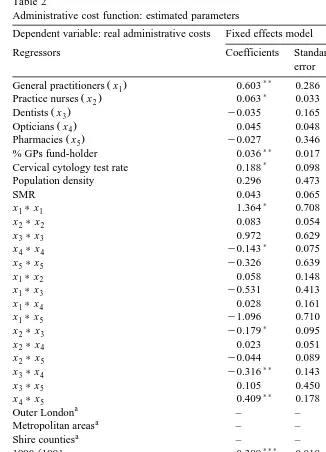
Table 2 reports the estimates of the cost function 24 including the linear, quadratic and cross product terms.17 The estimated SCE is evaluated at the 1994r1995 means of the explanatory variables. Since the variables are standard-ised at their 1994r1995 means the estimated linear terms on the primary care practitioners are the elasticities of administrative cost with respect to the numbers of GPs, dentists etc.
The fixed effects model is reported in the first two columns and has positive and significant linear terms for general practitioners and practice nurses, the linear term for opticians is positive but not statistically significant and those for dentists and pharmacies are negative, though not significant.
The last two columns in Table 2 present the estimates of the random effects model. We argued in Section 2.6 that endogenous managerial effort implied that
Ž .
the random effects model was likely to be misspecified. The Hausman 1978 test indicates that the assumption that area effects are not correlated with the other regressors cannot be rejected and so the random effects model is appropriate. Even though random effects is the preferred specification we also report the results from the fixed effects specification for comparison.
The random effects model yields economically more sensible results since all the linear cost terms on the primary care practitioners are positive. Further, the random effects model produces more modest prediction errors because, unlike the fixed effects model, it does not have to sacrifice a large number of degrees of freedom in estimating area effects. This is important when assessing economies of scale or scope.
The model of managerial effort in Section 2.4 implies that effort will be correlated with the number of practitioners if the marginal cost of practitioners is
Ž .
reduced by managerial effort Ca x-0 and if the manager cares about
administra-Ž . Ž . Ž .
tive costs b1)0 . The assumed cost function is of the form Csf x, q h a
which implies Ca x-0. b1 reflects both managerial preferences and the incentive structure in primary care administration. Thus the fact that the Hausman test indicates that unobserved area effects which pick up the effects of unobserved managerial effort are not correlated with the regressors including the numbers of practitioners may suggest that incentives to reduce primary care administration costs are weak.
Both models indicate that the number of general practitioners has the largest proportionate effect on costs. This is plausible since the remuneration system for GPs is much more complicated than for other practitioners. Density of population is significantly positively associated with administrative costs in the random
17
The value of lwas chosen to maximise the log-likelihood of the regression and was determined
Ž .
A. Giuffrida et al.rJournal of Health Economics 19 2000 983–1006 999
effects model. Since the variable shows relatively little change over time it may be picking up area effects. One possibility is that more densely populated areas have greater turnover of patients on GP lists and so generate more administration. The regional dummies are also of the expected sign, indicating that Inner London areas have significantly higher administrative costs than more rural areas and also than other urban areas, probably because of differences in property rents.
4.1. Economies of scale
Both models suggest that there are economies of scale in the administration of primary care. The fixed effects model estimates that the SCE is equal to 1.543 but this is not significantly different from unity. The random effects model estimate
Ž .
indicates a more modest SCE 1.209 which is statistically different from unity because the random effects estimates are more precise. The random effects model this suggests that there are economies of scale to be exploited at the mean 1994r1995 size of FHSAs.
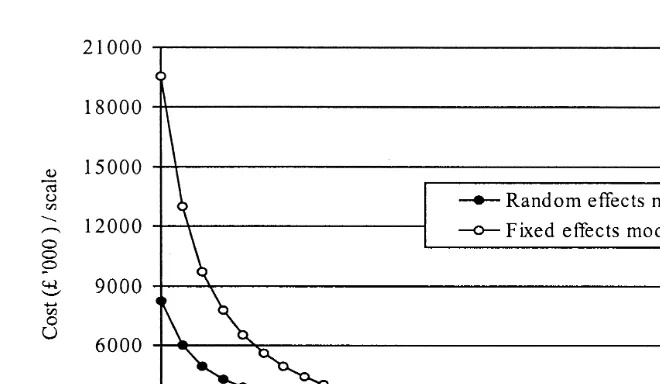
Fig. 1 illustrates the impact of scale on costs for non-local variations in scale. It is derived by calculating the administrative cost of an FHSA from the fixed and random effects models when the primary care practitioner variables are increased or decreased proportionately from their mean 1994r1995 values and the values of all other explanatory variables are held constant at their 1994r1995 means. The curves plot the resulting total costs divided by the scale factor for the primary care practitioner variables and can be regarded as the multi-output analogue of a single output average cost function.
The curve derived from the fixed effect model isAUB shape and indicates the presence of economies of scale for small and medium-sized FHSAs. Economies of scale are exhausted at a level 20% larger than the average FHSA.
The average cost curve estimated by the random effects model is similar to the fixed effects model for scales of production near to the mean. Economies of scale are much less for small FHSAs. The random effects model suggests that there are economies of scale at all level of production.
The fact that both models suggest marked economies of scale for small FHSAs may have some implications for possible future developments in the administra-tion of primary care in England. The NHS was reorganised around Primary Care
Ž .
Groups PCGs April 1999. PCGs consist of around 50 general practitioners with total lists of about 100,000 patients — they are about one fifth the size of FHSAs, some of whose functions they have taken over. Our estimates suggest that there could be adverse consequences for administrative costs if PCGs take over all of the primary care administrative tasks previously carried out by FHSAs.
4.2. Economies of scope
Fig. 1. Estimated average cost curve.
ŽBaumol et al., 1982 . One way to measure economies of scope is as the.
proportionate change in costs from partitioning the practitioner types into two
Ž .
groups Fournier and Mitchell, 1992 :
C x
Ž
1,0,P.
qC 0, xŽ
2,P.
yC xŽ
1, x2,P.
27
Ž
.
1 2
C x , x ,
Ž
P.
where x1, x2 is a partition of the practitioner vector.
We tested for economies of scope with six partitions: each practitioner type separately administered from the rest and practice nurses and GPs administered separately from all other practitioners. None of the cost differences from the fixed effect specification were significant and with the random effect specification only that for separate administration of practice nurses was significant.
4.3. Fundholding and administration costs
The introduction of fundholding in April 1991 increased the tasks which FHSAs were expected to carry out. The regression indicates that fundholding had
Notes to table 2:
a
These variables are not included in the fixed effects model as they are time invariant.
b Ž .
The Breush and Pagan test that Var ui s0.
A. Giuffrida et al.rJournal of Health Economics 19 2000 983–1006 1001 Table 2
Administrative cost function: estimated parameters
Dependent variable: real administrative costs Fixed effects model Random effects model
Regressors Coefficients Standard Coefficients Standard
error error
)) )))
Ž .
General practitioners x1 0.603 0.286 0.650 0.102
) )
Ž .
Practice nurses x2 0.063 0.033 0.066 0.034
Ž .
Dentists x3 y0.035 0.165 0.009 0.069
)))
Ž .
Opticians x4 0.045 0.048 0.084 0.032
Ž .
Pharmacies x5 y0.027 0.346 0.019 0.082
)) )))
% GPs fund-holder 0.036 0.017 0.046 0.016
)
Cervical cytology test rate 0.188 0.098 0.057 0.097
)))
Population density 0.296 0.473 0.055 0.019
SMR 0.043 0.065 0.061 0.073
)
x1)x1 1.364 0.708 y0.033 0.340
x2)x2 0.083 0.054 0.065 0.066
x3)x3 0.972 0.629 y0.296 0.349
) )))
x4)x4 y0.143 0.075 y0.312 0.075
x5)x5 y0.326 0.639 y0.351 0.365
x1)x2 0.058 0.148 y0.052 0.124
x1)x3 y0.531 0.413 y0.008 0.284
)
x1)x4 0.028 0.161 y0.248 0.139
x1)x5 y1.096 0.710 y0.096 0.289
)
x2)x3 y0.179 0.095 y0.090 0.086
x2)x4 0.023 0.051 0.045 0.055
x2)x5 y0.044 0.089 y0.029 0.085
))
x3)x4 y0.316 0.143 0.145 0.125
x3)x5 0.105 0.450 0.322 0.250
)) ))
x4)x5 0.409 0.178 0.259 0.127
a )
Outer London – – y0.106 0.054
a )))
Metropolitan areas – – y0.172 0.057
a )))
Shire counties – – y0.261 0.071
))) )))
1990r1991 0.389 0.018 0.388 0.019
))) )))
1991r1992 0.554 0.021 0.556 0.022
))) )))
1992r1993 0.633 0.024 0.632 0.025
))) )))
1993r1994 0.731 0.026 0.726 0.025
))) )))
1994r1995 0.806 0.027 0.797 0.026
)))
Intercept 7.026 0.238 7.156 0.063
l 1.04 1.04
Estimated SCE 1.543 1.209
2
w Ž .x
Hausman test x 29 6.26 –
2
R 0.929 0.925
w Ž .x
RESET F 3, 418 0.96 0.10
)))
w Ž .x
F-test that all uis0 F 89, 421 4.80 –
2 b )))
w Ž .x
Breush–Pagan test x 1 – 96.31
)))
w Ž .x
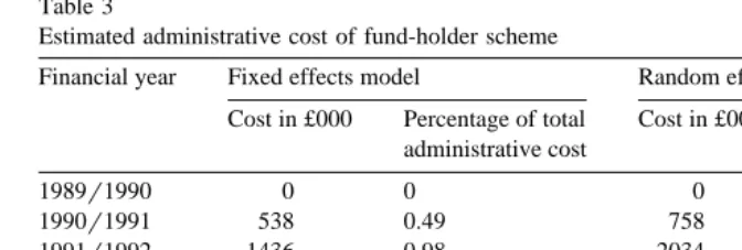
Table 3
Estimated administrative cost of fund-holder scheme
Financial year Fixed effects model Random effects model
Cost in £000 Percentage of total Cost in £000 Percentage of total administrative cost administrative cost
1989r1990 0 0 0 0
1990r1991 538 0.49 758 0.61
1991r1992 1436 0.98 2034 1.22
1992r1993 3690 2.17 5227 2.67
1993r1994 5943 2.95 8427 3.59
1994r1995 7770 3.55 11,009 4.30
Total 19,378 2.11 27,454 2.60
a significant positive effect on costs, though its magnitude is small. Table 3 presents the estimated administrative costs associated with fundholding both in absolute terms and as a proportion of total administrative costs. Fundholding accounts for 3.5–4.3% of the expenditure on administration in 1994r1995.
4.4. RelatiÕe efficiency
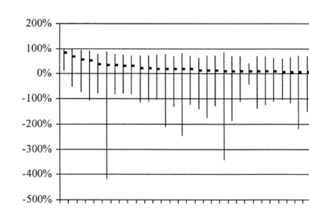
The estimated cost function can be used to derive an estimate of the difference in costs due to unobserved area effects, using the estimated fixed effects or, in the case of the random effects model, from the area residuals. We calculate the cost effect as the percentage difference between the cost of the area given its estimated fixed effect and the cost it would have with the area average fixed effect:
4
exp FiyF where F is the estimated area fixed effect and F is the mean fixedi
effect. Fig. 2 presents aAleague tableB for areas with above average fixed effects and plots the estimated area cost effects and their confidence intervals.
Ž
Such area effects have been interpreted as an indicator of efficiency Schmidt
.
and Sickles, 1984 but we argued in Section 2.5 that necessary conditions for this
Ž
interpretation are that all the regressors such as the number of primary care
.
practitioners and the quality of primary care are exogenous as far as managers are concerned and the effort of managers has negligible social cost. Even if these conditions are satisfied we showed in Section 2.6 that the area effects would yield biased estimates of the differences in managerial effort.
The size of the confidence intervals also indicates that one should be extremely cautious in using these results to label areas as more or less efficient in terms of their administrative costs.18Fig. 2 shows that only one of the
AinefficientB or high cost FHSAs have a cost effect which is significantly above the mean. The fact that there is little difference in estimatedAefficiencyB scores does not mean that there
18 Ž
The 95% confidence intervals are estimated by bootstrapping with 500 iterations Ai and Norton,
.
A. Giuffrida et al.rJournal of Health Economics 19 2000 983–1006 1003
Fig. 2. Estimated cost effects for higher cost FHSAs.
was no inefficiency since the scores are relative to the best, but still inefficient, area.
4.5. Changes in administratiÕe costs oÕer time
Administrative costs changes over time for three reasons: changes in the cost
Ž .
drivers outputs, quality and control variables ; changes in the price of inputs; and
Ž
shifts in the cost function across all FHSAs reflected in the year dummies in
.
[image:21.595.48.386.444.544.2]Table 2 . The first column in Table 4 shows the proportionate change in the cost each year. The second column is the change in costs which would have occurred
Table 4
Estimated breakdown of changes in administrative costsa
Financial year Percentage Percentage change due to
change in shift in changes in changes
administrative the cost explanatory in input
cost function variables prices
1989r1990–1990r1991 61 47.51 y0.36 9.70
1990r1991–1991r1992 33 18.01 2.22 10.24
1991r1992–1992r1993 17 8.20 2.19 6.21
1992r1993–1993r1994 20 10.25 2.15 6.15
1993r1994–1994r1995 9 7.78 0.91 0.39
a
due solely to the shift in the cost function with the regressors and input prices held constant. The third and fourth columns give the proportionate changes in costs which would be attributable solely to changes in the regressors and in the input prices respectively. It is apparent that the changes in the number of practitioners, quality levels etc have had relatively little effect on total cost over the period. The effect of input price inflation is greater but still minor compared with the shifts in the cost function.
The shift of the cost function over time could be the reflection of the following number of factors.
Ž .i There may have beenAnegative technical progressB: the technology altered to make it more costly to administer primary care. This seems implausible.
Ž .ii Factor price changes may have not been fully allowed for in our deflation of administrative costs by input price indices. Our input price index is imperfect but it is difficult to believe that there were increases in the prices of inputs used in administering primary care which are capable of explaining the more than doubling of administrative costs over the period.
Ž .iii An increase in the administrative tasks performed by FHSAs. The fund-holding variable is a direct measure of some of the new administrative tasks associated with the internal market and is included in the cost drivers. Since other additional administrative tasks were not associated with fundholding, the fundhold-ing variable may be an inadequate proxy for all the increased tasks resultfundhold-ing from the internal market reforms of the early 1990ies.
Ž .
Total administrative costs of FHSA were £215M in 1994r1995 current prices and we estimate that cost increased between 1989r1990 and 1994r1995 by 123% as a result of shift in the cost function, rather than changes in its arguments. Although the shift in the cost function may not be due to the 1990 reforms, these were the most obvious change in the FHSA environment in this period and no other factors suggest themselves. If the year dummies are picking up the effect of the increase in administrative tasks, we have identified a further large cost of the 1990 reforms.
5. Conclusion
We have presented a simple theoretical model of managerial effort to reduce
Ž
administrative costs which reinforces and extends previous cautions Newhouse,
.
A. Giuffrida et al.rJournal of Health Economics 19 2000 983–1006 1005
Our investigation of the costs of administering primary care in the NHS suggests:
Ø numbers of general practitioners had the greatest effect on administration costs
Ø there were unexploited economies of scale in primary care administration
Ø the introduction of fundholding had a significant but small positive impact on costs
Ø FHSA managers did not appear to be influencing either the quality of primary care or the proportion of fundholding practices
Ø most of the doubling of costs over the period 1989r1990–1994r1995 is attributable to shifts in the cost function, most likely reflecting unmeasured increases in administrative tasks, including those following the changes to the GP contract in 1990
The estimated efficiency scores are measures of performance relative to the best, but still inefficient, area. Only one area was significantly more expensive than average. This suggests that policy to reduce administration costs should be directed at improving the performance of all areas rather than concentrating attention on a few high cost areas.
Acknowledgements
Support from the Department of Health to the NPCRDC is acknowledged. The views expressed are those of the authors and not necessarily those of the Department of Health. We are grateful to Massimo Filippini, Gennaro Scarfiglieri and Tony Scott for helpful comments.
References
Ai, C., Norton, E.C., 1999. Standard errors for the retransformation problem with heteroscedasticity. 8th European Workshop on Econometrics and Health Economics, University of Catania, Septem-ber.
Armitage, P., Berry, G., 1994. Statistical Methods in Medical Research. Blackwell Science, Oxford. Arellano, M., 1987. Computing robust standard errors for within-group estimators. Oxford Bulletin of
Economics and Statistics 49, 431–434.
Baltagi, B.H., 1995. Econometric Analysis of Panel Data. Wiley, Chichester.
Baines, D.L., Whynes, D.K., 1996. Selection bias in GP fundholding. Health Economics 5, 129–140. Baumol, W., Panzar, I., Willig, R., 1982. Contestable Markets and the Theory of Industry Structure.
Harcourt Brace Janovich, San Diego, CA.
Caves, D.W., Christensen, L.R., Tretheway, M.W., 1980. Flexible cost functions for multiproducts firms. Review of Economics and Statistics 62, 477–481.
Davidson, R., MacKinnon, J.G., 1993. Estimation and Inference in Econometrics. Oxford Univ. Press, New York.
Department of Employment, several years. New Earnings Survey. HMSO, London.
Department of Health, 1997. The New NHS Modern and Dependable. The Stationery Office, London. Dor, A., 1994. Non-minimum cost functions and the stochastic frontier: on applications to health care
providers. Journal of Health Economics 13, 329–334.
Dor, A., Farley, D.E., 1996. Payment source and the cost of hospital care: evidence from a multiproduct cost function with multiple payers. Journal of Health Economics 15, 1–21. Ellis, R.P., 1998. Creaming, skimming and dumping: provider competition on the intensive and
Ž .
extensive margins. Journal of Health Economics 17 5 , 537–556.
Fournier, G.M., Mitchell, J.M., 1992. Hospital costs and competition for services: a multiproduct analysis. Review of Economics and Statistics 72, 627–634.
Fry, J., 1993. General Practice: the Facts. Radcliffe Medical Press, Oxford.
Gaynor, M., Pauly, M.V., 1990. Compensation and productive efficiency in partnerships: evidence from medical group practice. Journal of Political Economy 98, 544–573.
Godfrey, L.G., Hutton, J.P., 1994. Discriminating between errors-in-variables, simultaneity and mis-specification in linear regression models. Economics Letters 44, 359–364.
Halonen, M., Propper, C., 1999. The organisation of government bureaucracies: the choice between competition and single agency, mimeo, University of Bristol, May.
Hausman, J.A., 1978. Specification tests in econometrics. Econometrica 46, 1251–1271.
Levitt, R., Wall, A., Appleby, J., 1995. The Reorganised National Health Service. 5th edn. Chapman & Hall, London.
Newhouse, J.P., 1994. Frontier estimation: how useful a tool for health economics? Journal of Health Economics 13, 317–322.
NHS Executive, 1998. The New NHS Modern and Dependable: A National Framework for Assessing Performance. Department of Health, London.
NHS Executive, various years. Health Service Indicators Handbook. Leeds.
Ž .
Niskanen, W.A., 1971. Bureaucracy and representative government Aldine, New York .
Schmidt, P., Sickles, R., 1984. Production frontiers and panel data. Journal of Business and Economic Statistics 2, 367–374.
Scott, A., Parkin, D., 1995. Investigating hospital efficiency in the new NHS: the role of the translog cost function. Health Economics 4, 467–478.
Skinner, J., 1994. What do stochastic frontier cost functions tell us about inefficiency? Journal of Health Economics 13, 323–328.
Wholey, D., Feldman, R., Christianson, J.B., Enberg, J., 1996. Scale and scope economies among health maintenance organizations. Journal of Health Economics 15, 657–684.
Ž .