Structure Across International Equity Markets
Kevin Bracker and Paul D. Koch
This study investigates whether, how, and why the matrix of correlations across interna-tional equity markets changes over time. A theoretical model is proposed to specify potential economic determinants of this correlation structure. The empirical validity of this economic model is investigated by employing daily returns for different national stock indexes, from 1972 through 1993, to construct a quarterly time series of the correlation matrix. This quarterly time series is used to investigate the stability of the correlation matrix over time, and to estimate the economic model. The model is then applied to generate out-of-sample forecasts of the correlation structure. © 1999 Elsevier Science Inc.
Keywords:International market integration
JEL classification:F36, G15.
I. Introduction
The degree of capital market integration varies substantially across different pairs of national markets and over time. During some periods, there is less association between the economic health of countries in different sectors of the world economy. At such times, national equity markets tend to follow their own paths, and experience less comovement with other markets. At other times, there is greater association between the economic performance of different sectors of the world, especially across countries that are more interdependent through trade, and we observe greater comovement across respective national equity markets. Recently, we have witnessed occasional contagion effects whereby certain groups of national equity markets rally or crash together in response to economic and/or political events, exhibiting correlations that are temporarily very high.
This discussion describes evolution in the nature and extent of global capital market integration, characterized by dramatic changes over time in the correlation matrix across
Economics, Finance, and Banking (K.B.), Pittsburg State University, Pittsburg, Kansas, School of Business (P.D.K.), University of Kansas, Lawrence, Kansas, USA
Address correspondence to: Dr. P. D. Koch, School of Business, University of Kansas, Lawrence, KS 66045.
national equity returns. This study focuses on understanding, modeling, and forecasting dynamic movements in the correlation structure.1We hypothesize that greater economic integration across countries should lead to greater capital market integration. Interdepen-dence through trade and capital flows implies interdepenInterdepen-dence in investors’ valuation decisions across national equity markets. In this light, we suggest that pairs of countries experiencing greater economic integration should also experience greater comovement in their respective capital markets. Furthermore, as the nature and extent of economic integration across countries changes over time, we may expect concomitant changes in the degree of comovement across respective capital markets.
This study addresses whether, how, and why the correlation structure changes over time by testing the stability of the correlation matrix over different periods, and by modeling potential economic determinants of the correlation structure. The economic model is then applied to generate out-of-sample forecasts of the correlation structure. A better understanding of dynamic movements in the correlation structure is critical, given that this structure reflects the nature and extent of global market integration, and given its impact on the risk-return performance of international equity portfolios. In light of the recent precarious situation in world financial markets, the ability to predict changes in correlation patterns should be of interest to market participants, national policy makers, and regulatory bodies involved in monitoring and managing global market behavior.2
This study employs daily returns on ten national stock indexes, from 1972 through 1993, to construct a quarterly time series of the correlation matrix. This time series embodies any variation in the correlation structure experienced over the sample, and is used to test formally the hypothesis that the correlation matrix does not change over time. Results reveal substantive changes over both short and long time horizons throughout this 22-year sample period. Augmented Dickey–Fuller tests indicate that almost all of these time series of pairwise correlations contain no unit root. This outcome alleviates concern about possible spurious relationships with economic variables. This battery of stability tests provides evidence of the dramatic evolution in the correlation matrix, and motivates the need to further analyze potential economic determinants of the correlation structure. We seek to gain a better understanding of these dynamic changes in the correlation structure by modeling economic factors that may influence the degree of comovement across equity markets. We hypothesize that the degree of integration across international capital markets at any point in time depends upon the degree of economic integration
1Throughout this study, the termcorrelation structurerefers to the matrix of correlations across returns in
different national equity indexes. This correlation structure characterizes the nature and extent of integration across different pairs of national equity markets. Dynamic changes in the correlation structure imply changes in the risk-return performance of international equity portfolios over time. For a summary of the role of the correlation structure in international diversification, see Haugen (1990, pp. 134–136), Isimbabi (1992), and Hatch and Resnick (1993). For more related work on the nature and extent of international market integration, see Arshanapalli and Doukas (1993), Bachman et al. (1996), Eun and Resnick (1984), Kasa (1992), and Longin and Solnik (1995).
2Changes in the correlation matrix, along with changes in expected returns and variances across national
across the countries involved.3We develop a theoretical model in which each time series of pairwise correlations may depend upon factors that characterize and influence the extent of economic integration across the two markets in question. The set of all such pairwise equations is then estimated both as a pooled regression and as a system of seemingly unrelated regressions that describes potential economic determinants of the correlation structure. This analysis is conducted on the subset of seven countries for which complete economic data are available. Results indicate that the degree of international integration (the magnitude of the correlations) is positively associated with (1) world market volatility and (2) a trend; while it is negatively related to (3) exchange rate volatility, (4) term structure differentials across markets, (5) real interest rate differentials, and (6) the return on a world market index.
This analysis sheds light on the economic forces that influence the correlation structure over time, and thus the evolution in global capital market integration. For example, these results corroborate a priori expectations that divergent macroeconomic behavior across countries tends to be associated with divergent behavior across national equity markets, resulting in lower market correlations. In addition, the influence of economic factors (1) and (6) listed above indicate an increase in comovement across international equity markets when world markets are more volatile and/or falling. This outcome suggests a decline in the risk-reduction benefits of international diversification at the very time when these benefits are needed most.
Finally, the economic model is employed to generate out-of-sample forecasts of the correlation structure. The forecast performance of this model dominates that of other atheoretical models which ignore economic determinants of the correlation structure. This outcome adds credence to the validity of the theoretical economic model, and suggests that modeling the correlation structure holds promise in assisting managers to exploit inter-national investment opportunities.
The paper proceeds as follows. Section II reviews the literature on stability in the correlation structure, discusses the data, and presents the stability tests. Section III develops the theoretical model describing economic determinants of the correlation structure, and Section IV estimates the model. Section V compares the forecast perfor-mance of this model with respect to alternative forecasting techniques. A final section summarizes and concludes.
II. Literature Review, Stock Market Data, and Stability Tests
Literature Review
The existing literature offers mixed evidence on the stability of the correlation structure. Several earlier studies by Panton et al. (1976), Watson (1980), and Philippatos et al. (1983) all find support for stable relationships across national equity markets. In contrast, Makridakis and Wheelwright (1974), Haney and Lloyd (1978), Maldonado and Saunders (1981), Fischer and Palasvirta (1990), Madura and Soenen (1992), Wahab and Lashgari (1993), and Longin and Solnik (1995) argue that the relationships are unstable. Falling somewhere between these two camps, Kaplanis (1988) suggests that correlations are stable while covariances are unstable; Marcus et al. (1991) suggest that the holding period
3For other studies that motivate this hypothesis, see Arshanapalli and Doukas (1993), Bachman et al. (1996),
analyzed has a bearing on the correlation structure observed; and Meric and Meric (1989) find instability for shorter periods, offset by stability over longer periods.
The disparity in results across this literature is presumably attributable to the wide range of sample periods and sampling frequencies examined, as well as different meth-odologies employed.4Interestingly, most recent studies tend to find greater instability, suggesting that interrelationships among national stock markets may have undergone a substantive change during the 1980s.
Stock Market Data
The data include Morgan Stanley Capital International’s daily closing stock index values for ten national markets (Australia, Canada, Germany, Hong Kong, Japan, Mexico, Singapore, Switzerland, the United Kingdom, and the United States), as well as daily bilateral exchange rates between the US dollar and the nine other currencies, from 1972 through 1993.5 The analysis is applied to daily returns for every national market, denominated both in US dollars and in the home currency.
Tests for Stability in the Correlation Matrix
From these time series of daily stock returns, we compute the correlation between every pair of national markets over each quarter during this 22-year sample period. The resulting time series of 88 quarterly observations on the correlation matrix reveals the nature and extent of changes in the correlation structure over time. This quarterly time series is then employed to test for stability in the correlation structure, using a Jennrich (1970) test for the equality of two correlation matrices.6
Table 1 presents the results of three different approaches for investigating the hypoth-esis that the correlation matrix does not change over time. First, we examine the null hypothesis that the correlation matrix does not change from one quarter to the next, across each of the 88 quarters in the sample period. Panel A of Table 1 presents the frequency of rejections out of these 87 tests comparing consecutive quarterly correlation matrices. If the correlation matrix is truly constant, we would expect approximatelyninerejections out of 87 tests at the 0.10 level of significance (along withfiverejections at the 0.05 level and
one rejection at the 0.01 level). Panel A reveals that stability is rejected far more
4Different studies in this literature employ data: (1) taken over different sample periods which sometimes
extend prior to the early 1970s, when world equity and currency markets were more stable, and (2) taken at different frequencies (daily, weekly, monthly, quarterly, or annually).
5Morgan Stanley Capital International (MSCI) data on individual firm stocks around the world represent
approximately 60% of the world’s total market capitalization. From these data MSCI constructs national stock indexes that are fully comparable. The ten national equity markets chosen for this analysis account for approximately 90% of the world’s total market capitalization.
6Appendix A provides the formal Jennrich (1970) test. Data for Mexico are unavailable prior to 1988.
Therefore, stability tests where both periods tested begin after 1988 use all ten countries. Otherwise only nine countries are employed.
Table 1. Jennrich Tests for Equality of Two Correlation Matrices.a
Pearson correlations are estimated from daily returns in U.S. dollars across ten national markets, for each quarter throughout the 22-year period, 1972–1993. The result is a time series that embodies quarterly movements in the correlation matrix across national equity markets.
The Jennrich (1970) test is applied to investigate the equality of: A: consecutive quarterly correlation matrices;
B: nonconsecutive quarterly correlation matrices (one, two, and three quarters apart); C: consecutive correlation matrices estimated over time intervals longer than one quarter.
This Table presents the frequency of rejections in applying these Jennrich (1970) tests.b
Panel A: Frequency of Rejections Across Consecutive Quarterly Correlation Matrices
Panel A
10% Level
(12p)5.10
5% Level
(12p)5.05
1% Level
(12p)5.01
Number of times that equality is rejected out of 87 Tests
39*** 29*** 13***
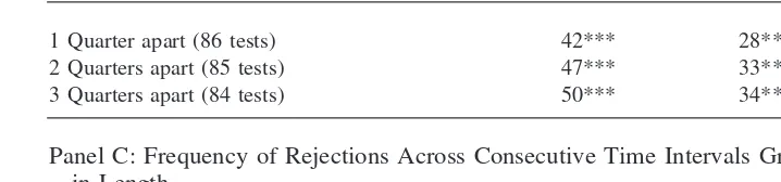
Panel B: Frequency of Rejections Across Non-Consecutive Quarterly Correlation Matrices
Panel B: 10% Level 5% Level 1% Level
1 Quarter apart (86 tests) 42*** 28*** 18***
2 Quarters apart (85 tests) 47*** 33*** 16***
3 Quarters apart (84 tests) 50*** 34*** 23***
Panel C: Frequency of Rejections Across Consecutive Time Intervals Greater than One Quarter in Length
Panel C: 10% Level 5% Level 1% Level
Semiannual (43 tests) 33*** 22*** 16***
Annual (21 tests) 20*** 19*** 16***
Biannual (10 tests) 10*** 10*** 9***
Five-and-one-half years (3 tests) 3 3 3
Eleven years (1 test) 1 1 1
aJennrich (1970) provides a Chi-square statistic to test the equality of two correlation matrices; details appear in Appendix A. bResults are robust with respect to the use of Spearman correlations, home currency returns, and the alternative Box M test
for equality across correlation matrices.
*** Indicates that the number of rejections is greater than expected by chance 1% of the time, within a binomial framework that bases the probability of acceptance for each individual test atp(5.90, .95, and .99), and the probability of rejection at 1-p
(5.10, .05, and .01). Therefore, (12p) represents the significance level for each individual test. This binomial analysis is not applied to the last two rows in Panel C due to the small number of tests conducted in each case.
frequently than is expected by chance (39rejections at the 0.10 level,29rejections at the 0.05 level, and13rejections at the 0.01 level).
We can more formally address the issue of whether the number of rejections docu-mented in Table 1 is “significantly greater than expected” (at each level of significance), by considering the outcome of every test as being drawn independently from a binomial distribution. If we consider an acceptance of the null in one trial to be a success, and a rejection to be a failure, then at the 10% level of significance the probability of success for that trial is .90 and the probability of failure is .10. By viewing the sequence of tests this way, we can determine the “critical values” for the number of rejections expected at the 10%, 5%, and 1% significance levels. Given a probability of success at p5.90 (the 10% level of significance), with 87 independent tests there is less than a 1% chance of rejecting the null more thansixteentimes. Similarly, given a probability of success atp5 .95, there is less than a 1% chance of rejecting the null more thantentimes. Finally, given a probability of success atp5.99, there is less than a 1% chance of rejecting the null more thanfourtimes. Once again, because the numbers in Panel A of Table 1 are greater than these respective “critical values,” the number of rejections in each cell of Panel A is greater than would be expected 1% of the time, under this binomial exercise.
Next, we consider the possibility that these quarterly correlation matrices may change more slowly over time, by investigating the equality of correlation matrices that are one, two, and three quarters apart. Panel B of Table 1 presents the frequency of rejections across nonconsecutive quarterly correlation matrices, and once again reveals far more rejections than could be expected by chance. Finally, Panel C considers the stability of the correlation matrix computed over longer time intervals of 6 months, 1 year, 2 years, 51⁄2 years, and 11 years. Results in Panel C uniformly indicate instability over these longer time periods as well.
While our results are consistent with most recent studies on this issue, these latter findings contrast with the results of Meric and Meric (1989), which suggest some underlying long-run stability in the correlation matrix. This contrast is important. If there were truly long-run stability, then the short-run instability documented in Panels A and B of Table 1 would not be critical for long-term investors. Instead, our results overwhelmingly indicate significant changes in the correlation matrix over both short and long time horizons. These results provoke the question as tohowandwhythe correlation structure varies over time. Before we proceed to address this question by developing the economic model, we must investigate whether each time series of pairwise correlations contains a unit root. If changes in the correlation structure contain a unit root (follow some form of random walk), then our model of the correlation structure may result in identifying spurious relationships with economic variables (Enders 1995).
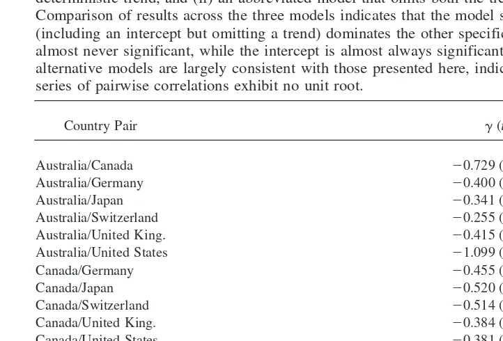
In this light, we perform Augmented Dickey–Fuller (ADF) tests on each time series of quarterly pairwise correlations. Results are provided in Table 2 and indicate rejection of the unit root hypothesis for 18 of the 21 time series of pairwise correlations, at the .10 level or better. Because the vast majority of these time series have no unit root, it is reasonable to proceed with our attempt to model how and why the correlation structure changes over time.
(See, for example, Gultekin, 1993; Solnik, 1983; Chen et al., 1986; Bodurtha et al., 1989; Campbell and Hamao, 1992). These studies suggest the following country-specific factors as possible determinants of national equity returns:
INDit 5 industrial production growth in countryiduring quartert;
INFLit 5 inflation in country iduring quartert; Table 2. Augmented Dickey-Fuller (ADF) Tests
This table presents the results of ADF tests that investigate the existence of a unit root in the time series of quarterly correlation coefficients for each pair of national equity markets.
The regression model used to conduct the ADF test is specified as follows:
Dcorrt5a01gcorrt211b1(Dcorrt21)1b2(Dcorrt22)1«t.
Under H0:g50, there is a unit root. Therefore a rejection of Ho:g50 indicates no unit root.
Results indicate no unit root (rejection of Ho) for 18 of the 21 time series of correlations.
Lagged changes in the correlation coefficient beyond two quarterly lags are insignificant. This analysis includes 88 quarters, but only 85 observations are used due to the two quarterly lags. Statistical significance is based on critical values generated from a conservative sample size of 50 observations (significance levels based on a sample size of 100 do not alter the results.)
We have also conducted unit root tests using: (i) an expanded model that includes a deterministic trend, and (ii) an abbreviated model that omits both the trend and the intercept. Comparison of results across the three models indicates that the model specified above (including an intercept but omitting a trend) dominates the other specifications. The trend is almost never significant, while the intercept is almost always significant. Results for both alternative models are largely consistent with those presented here, indicating that most time series of pairwise correlations exhibit no unit root.
Country Pair g(tratio)
Australia/Canada 20.729 (24.007)***
Australia/Germany 20.400 (22.904)*
Australia/Japan 20.341 (22.648)*
Australia/Switzerland 20.255 (22.197)
Australia/United King. 20.415 (23.155)**
Australia/United States 21.099 (25.624)***
Canada/Germany 20.455 (22.966)**
Canada/Japan 20.520 (23.463)**
Canada/Switzerland 20.514 (23.299)**
Canada/United King. 20.384 (22.990)**
Canada/United States 20.381 (22.634)*
Germany/Japan 20.311 (22.700)*
Germany/Switzerland 20.324 (22.971)**
Germany/United King. 20.299 (23.162)**
Germany/United States 20.619 (23.868)***
Japan/Switzerland 20.255 (22.473)
Japan/United King. 20.332 (22.917)*
Japan/United States 20.671 (23.868)***
Switzerland/Unit. King. 20.233 (22.473)
Switzerland/United St. 20.748 (24.379)***
United King./United St. 20.551 (23.963)***
INTit 5 real interest rate in countryiduring quartert;
LOSHit 5 term structure premium in countryiduring quartert;
7
SIZEit 5 share of total world market capitalization in countryiduring quartert;
The economic rationale for hypothesizing that these variables are among the determinants of national stock returns is grounded in the discounted cash flow model. The first four variables listed above represent different aspects of a country’s macroeconomic perfor-mance that affect expected cash flows and/or discount rates in that national market, and thus have a bearing on the market’s expected returns. The last variable listed above is motivated by the well-documented size effect within a national market, whereby higher discount rates are demanded for smaller firms (Keim 1983; Reinganum 1983). Potential explanations for this firm-size effect include greater information costs, transaction costs, and less liquidity associated with trading equity in smaller firms. By extension, we suggest that the relative size of a national equity market may also have a bearing on that country’s equity returns, due to greater information costs, transaction costs, and less liquidity associated with trading equity in smaller national markets.
While this discussion serves to motivate potential macroeconomic determinants of the first moment (expected returns) across different elements in the vector of national equity returns, we are interested in modeling determinants of the second moment (the correlation structure).8As a first step, we postulate that the extent of comovement between a pair of national markets may depend upon the extent to which these five macroeconomic variables diverge across the two markets, as follows:
rijt5b01b1uINDi2INDjut1b2uINFLi2INFLjut1b3uINTi2INTjut
1b4uLOSHi2LOSHjut1b5uSIZEi2SIZEjut1eijt, (1)
where
rijt 5 estimated correlation between daily returns in countriesiandjduring quartert;
eijt 5 disturbance term, assumed to beiid N(0, s
2 ).
Generally if there is greater divergence in macroeconomic behavior across countries, we expect less comovement across equity markets, implying negative coefficients forb1–b5.
9
7The term structure premium is defined as the difference between long term and short term government bond
rates in countryiduring quartert(Chen et al., 1986). This difference is a measure of the premium demanded
for long term investments in a country.
8For other work that motivates and investigates this issue, see Arshanapalli and Doukas (1993), Bachman
et al. (1996), Bodurtha et al. (1989), Campbell and Hamao (1992), Roll (1992), and Bracker et al. (1999).
9The recent convergence in various aspects of macroeconomic behavior across European Union member
countries (such as interest rates and inflation rates), as specified in the Maastricht treaty, serves to illustrate and motivate the spirit of our theoretical specification in Equation 1.
The empirical validity of this specification requires some attention. Note that Equation 1 constrains each
macroeconomic variable to enter the model as the absolute differential in behavior across marketsiandj, during
quartert. It is conceivable, however, that each variable in countryihas a substantive influence on the correlation, independent of the analogous factor in countryj. That is, it may be more appropriate to allow each factor in both countries to enter the regression model independently, rather than in the form of an absolute differential, as follows:
rijt5a01a1INDit1a2INDjt1a3INFLit1a4INFLjt1a5INTit1a6INTjt1a7LOSHit1a8LOSHjt
1a9SIZEit1a10SIZEjt1eijt.
In addition to motivating the potential influence of the above five macroeconomic differentials on rijt, the discounted cash flow model further motivates expansion of
Equation 1 to incorporate five additional macroeconomic variables that may also directly influence international correlations.
First, bilateral trade conditions may impact national equity index returns for a given pair of trading partners (Bodurtha et al., 1989). As exports from economyito economy
j (Xij) increase, higher cash flows should be expected into country i. In contrast, the
imports of economyifrom economyj(Mij) may have the opposite effect on cash flows
for countryi’s firms. In this light, changes in the absolute magnitude of the trade balance between two economies (uXij2Miju) should positively influence one economy and stock
market, while negatively influencing the other, to exert a negative impact on the corre-lation,rijt. The extent of this impact, however, should reflect the degree of importance of
this bilateral trade activity with respect to aggregate economic activity in each national market involved. If this bilateral trade balance reflects a small proportion of Gross Domestic Product (GDP) for one of the two countries, it is not likely to exert much influence on that country’s stock market. On the other hand, if the trade balance represents a large proportion of GDP foronecountry, we may expect a substantive impact on stock returns in that country, and thus a substantive response inrij. Furthermore, if uXij2Miju
represents a large proportion of GDP for both countries, we would expect a greater response inrij. In this light we construct the following variable to incorporate the potential
influence of the trade gap onrij, from the point of view of both countries:
GAPij5~uXij2Miju!/GDPi1~uXij2Miju!/GDPj.
Second, this trade gap variable may not adequately reflect the full impact of bilateral trade conditions on the correlation structure, because a given pair of countries may have a trade gap near zero while engaging in a substantial amount of trade. In this light, we also incorporate a second variable to account for the total amount of trade across the two countries:
TRADEij5~Xij1Mij!/GDPi1~Xij1Mij!/GDPj.
This variable emphasizes the notion that both exports and imports have a role in wealth creation, and may thus influence the interaction of national equity markets. Appendix B provides further insight into this specification of the GAPijand TRADEijvariables.
Third, absolute changes in the bilateral exchange rate (uXRCHiju) may influence the
trade conditions discussed above, and may thus also influence national equity returns in both countries. If the exchange rate changes by a larger percentage, then we expect a larger adjustment in bilateral trade conditions (with a lag) in favor of the depreciating
The model specified in (1) imposes the following constraints on the above model:
a15 2a2(5b1);a35 2a4(5b2);a55 2a6(5b3);a75 2a8(5b4);a95 2a10(5b5).
country. This observation suggests a potential indirect negative influence of absolute exchange rate changes on the correlation, through their impact on the trade gap.10
Fourth, volatility in the bilateral exchange rate (XRSDij) represents another source of
uncertainty which may dampen economic and equity market integration. If all countries’ returns are calculated on a US Dollar basis, each national return contains both an equity return component and a currency return component. As currency rates become more volatile, the currency component becomes more important relative to the equity return component. In this case, higher exchange rate volatility may be expected to dampen the correlation between different pairs of national equity market returns, denominated in US Dollars. This dampening effect should be less important across home currency returns that abstract from exchange rate movements.
Fifth, overall volatility across the world’s stock markets may influence the level of discount rates commanded around the world. As the variance of a world equity index (WLDVOL) increases, investors around the world may demand higher rates of return to compensate this risk, resulting in higher correlations across different pairs of national equity markets. Erb et al. (1994), Farrell (1997), Longin and Solnik (1995), and Solnik et al. (1996) all argue that world market volatility is an important determinant of correlations across national markets.
Finally, in addition to the above ten macroeconomic variables, we incorporate several additional factors that appear in anecdotal discussions of potential influences on the correlation structure, although they do not enter explicitly into the discounted cash flow model. First, Erb et al. (1994) observe that correlations tend to be low during times of general upward trends in world equity valuation, but that correlations become higher when stock returns are declining around the world. This observation suggests asymmetric behavior of the correlation structure in times of rising versus falling markets worldwide. In this light, the return on a world market portfolio (WLDMKT) may exhibit a negative association with the correlation structure over time. Second, evolution toward global capital market integration would suggest that correlations are trending upward over time due to factors such as greater interdependence across national economies, improved telecommunications technology, global deregulation of markets, more cross-listing of securities, growth in multinational activities, increasing international diversification, and so forth (Bachman et al., 1996; Kaplanis, 1988; Kasa, 1992; Longin and Solnik, 1995). This possibility is accounted for by incorporating a trend in the regression model. Third, these correlations were dramatically higher during October 1987 and October 1989, two periods of increased world market volatility (Roll, 1989). Thus, two dummy variables are incorporated to account for potentially aberrant behavior during the fourth quarters of 1987 and 1989, respectively. Fourth, it is well-documented that different national equity markets have experienced seasonal patterns in market activity and valuation. Meric and Meric (1989) further document that the correlation matrix is less stable during the summer
10It is important to note that the three variables,uINFL
i2INFLju,uINTi2INTju, anduXRCHiju, are related through international parity conditions (Eiteman et al., 1998). In fact, if purchasing power parity and interest rate parity were to hold perfectly in all periods, these three variables would be collinear. This situation may give cause for concern about potential multicollinearity in the regression model. However, we observe that it is
months. In this light, we account for potential seasonality in the correlation matrix by adding quarterly dummy variables.
The final regression model incorporates all of these influences, as follows:
rijt5b01b1uINDi2INDjut1b2uINFLi2INFLjut1b3uINTi2INTjut
1b4uLOSHi2LOSHjut1b5uSIZEi2SIZEjut1b6GAPijt1b7TRADEijt
1b8uXRCHijut1b9XRSDijt1b10WLDVOLt1b11WLDMKTt1b12TREND 1b13OCT871b14OCT891b15Q11b16Q21b17Q31eijt; (2)
wherei5 country 1 to 6;j 5country (i1 1) to 7;t 5quarter 1 to 88; INDit 5 Growth in industrial production in countryiduring quartert;
INFLit 5 Inflation Rate in countryiduring quartert;
INTit 5 Real interest rate (long term government rate-inflation rate) during
quarter t;
LOSHit 5 Spread between long and short term bond rates in country i during
quarter t;
SIZEit 5 Percent of world equity market share in marketiduring quartert;
GAPijt 5 (uXij2Mijut)/GDPit1(uXij2 Mijut)/GDPjt;
TRADEijt 5 (Xij 1Mij)t/GDPit1 (Xij1 Mij)t/GDPjt;
XRCHijt 5 Percent change in bilateral exchange rate during quartert;
XRSDijt 5 Standard Deviation in daily bilateral exchange rate during quartert;
WLDVOLt 5 Standard deviation of daily world stock market index return during
quarter t;
WLDMKTt 5 Percent change in world stock market index during quartert;
TREND 5 Nonlinear trend, ln(t);
OCT87(89) 5 Dummy variable equal to 1 in fourth quarter of 1987(1989); Q1, Q2, Q3 5 Seasonal Dummy variables for the first three quarters. Appendix C discusses data sources for the variables specified above.
IV. Estimation of the Economic Model
For three countries (Hong Kong, Mexico, and Singapore), daily stock market data and/or quarterly macroeconomic data are unavailable over a considerable portion of the sample period. Hence, these three countries are not included in the regression analysis. The remaining seven countries offer 21 distinct pairwise correlations. A different time series regression Equation 2 is specified for each such pairwise correlation.
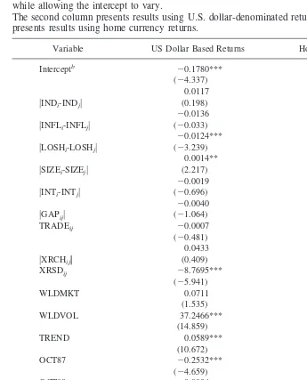
Table 3. Results of Pooled Time Series and Cross-Sectional Regression Analysisa
Equation 2 specifies the economic model describing quarterly time series movements in the correlation structure. The dependent variable is the bilateral correlation between national markets
iandj, computed from daily returns over each quarter throughout the period, 1972–1993. Complete quarterly economic data are available for seven countries. Hence, we specify a different equation to determine the correlation between each of the 21 possible pairs of these seven national markets. This table presents results of estimating this model as a pooled system, constraining the influence of each economic variable to be identical across all 21 equations, while allowing the intercept to vary.
The second column presents results using U.S. dollar-denominated returns. The third column presents results using home currency returns.
Variable US Dollar Based Returns Home-Currency Returns
Results of the Pooled Regression Model
Pooled regression results are presented in Table 3 for both US Dollar-based data and home-currency returns. First, the goodness of fit statistics indicate that these economic determinants offer substantive explanatory power regarding time series movements in the correlation structure. Second, the intercept varies substantively across many of the 21 Table 3. (Continued)
Variable US dollar Based Returns Home-Currency Returns
AUSJAP 0.0652 0.0029
aA Cochrane–Orcutt transformation is employed to correct for first-order autocorrelation in the error term in (11). Results
are generally robust without this transformation.
bThis coefficient presents the intercept for the corrrelation between the US and UK markets. The remaining 20 pairwise
correlations are allowed to have intercepts that deviate from the US-UK intercept. The 20 coefficients that are presented following the model’s main parameters represent the difference between the intercept for each pair of markets and the intercept for the US and UK markets.
pairwise equations in the model. Third, economic variables that are significant at the 0.01 level for both US Dollar and home-currency returns include exchange rate volatility, world market volatility, the time trend, the October 1987 dummy variable, and a seasonal dummy for the third quarter. For US Dollar-denominated returns, two additional signif-icant explanatory variables appear in the differential in the term structure premium (uLOSHi2LOSHju) and the size differential (uSIZEi2SIZEju). Alternatively, for
home-currency returns, additional significant factors include the real interest differential (uINTi2INTju), the world market return (WLDMKT), and the October 1989 dummy. We
elaborate on the individual influence of each regression variable below in the discussion of the SUR model.
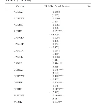
Results of the Seemingly Unrelated Regressions (SUR) Model
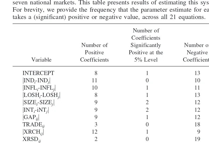
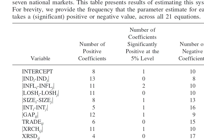
Estimation of the SUR model yields 17 parameter estimates for each of the 21 regression equations. To summarize the nature and strength of these results, we present the frequency that each parameter estimate takes on a (significant) positive or negative value across all 21 equations in Tables 4 and 5, for US Dollar-denominated returns and for home-currency returns, respectively.11
These SUR results largely corroborate the pooled results. First, for US Dollar returns in Table 4, economic variables that enter significantly across a substantial number of country pairs include (in order of their importance) world market volatility, the trend, exchange rate volatility, the real interest differential, the size differential, total trade, and the October 1987 dummy. For home currency returns in Table 5, analogous results point to world volatility, the trend, the real interest differential, the October 1987 dummy, the direction of world market returns, total trade, exchange rate volatility, and the term structure differential. We elaborate below.
The dominant factor in this analysis is world equity market volatility, which is significantly positive in all 21 equations. This is a reasonable result, given that greater volatility in the world index is likely to be associated with worldwide shocks that affect many markets (see Solnik et al. 1996).12
Exchange rate volatility also displays a stable dampening effect on the correlations across national equity markets. For US Dollar returns in Table 4, the coefficient for this variable is negative in 19 of 21 equations, and is statistically significant in 12 equations. In home currency returns (Table 5), this coefficient is negative in 17 equations but
11We have also re-estimated the model over two subsamples of equal length, to investigate the stability of
parameter estimates across this 22-year sample period. With the exception of the time trend, results are generally robust and are available upon request. The unstable trend in the correlation structure is discussed below.
12The return variance for any portfolio is, by definition, positively related to the return variances of its
components, as well as the covariances across all possible pairs of components. Due to the influence of covariances, we may expect a “definitional” relationship between world market volatility and the correlation structure acrossallnational markets.
significant in only three equations. Thus, as expected, this dampening effect appears less important for a portfolio that abstracts from exchange rate movements. It is noteworthy that the pooled results in Table 3 reveal a significant negative influence of exchange rate volatility, regardless of the adjustment for exchange rate movements.
The trend is positive in 20 equations, and significant in 12, on a US Dollar basis in Table 4. Similar results obtain for home-currency returns. This outcome supports a trend toward greater integration over time. On the other hand, re-estimation of the model over two equal subperiods reveals that this trend is predominantly in the first 11-year subpe-riod.13
13The specification of the trend variable as the natural log of the quarter (1 through 88) implies a more
pronounced trend over the first half of the 22-year sample period. When estimated over the second 11-year subperiod (1983–1993), this trend appears slightly negative for US dollar returns, or neutral for home-currency returns. A linear trend and piecewise linear trends (allowing the slope to change in the fourth quarter of 1985 or the fourth quarter of 1987) have also been investigated. The overall results (available upon request) are robust with respect to each specification. The observation that the trend is statistically significant when estimated over the entire collection of correlations in the pooled model and over the entire sample period, while it is insignificant for many bilateral pairs in the SUR model and over two 11-year subsamples, is consistent with the results of Bachman et al. (1996), Kasa (1992), and Solnik et al. (1996).
Table 4. Results of Seemingly Unrelated Regression (SUR) Analysis: US Dollar-Based Data
Equation 2 specifies the economic model describing quarterly time series movements in the correlation structure. The dependent variable is the bilateral correlation between national markets
iandj, computed from daily returns over each quarter throughout the period, 1972–1993. Complete quarterly economic data are available for seven countries. Hence, we specify a different equation to determine the correlation between each of the 21 possible pairs of these seven national markets. This table presents results of estimating this system as a SUR model. For brevity, we provide the frequency that the parameter estimate for each economic variable takes a (significant) positive or negative value, across all 21 equations.
The real interest differential reveals a negative influence on the correlation structure, especially for home currency returns. These results suggest that, as real interest rates diverge across two markets, stock returns also tend to diverge resulting in a lower correlation.
Greater trade flows between countries reflect greater economic integration, which may be expected to result in greater equity market integration. However, Tables 4 and 5 reveal a tendency for the total trade variable to display a negative influence on the correlation, which is counterintuitive. In contrast, the pooled regression in Table 3 reveals no significant relationship.
There is mixed evidence for the argument that two markets should display less correlation if they are more divergent in size. For US Dollar returns in Table 4, the coefficient on the size differential is negative 12 times (with five coefficients significant), while it is positive nine times (with two significant). Results are similar for home currency returns in Table 5. These results lean toward the argument that markets more disparate in size have lower correlations. In contrast, the pooled regression in Table 3 suggests a positive relationship between the size differential and the correlation structure.
The world market return exhibits a tendency for a negative relationship with the correlation structure, but only for returns stated on a home currency basis. In Table 5, this Table 5. Results of Seemingly Unrelated Regression (SUR) Analysis: Home Currency Data
Equation 2 specifies the economic model describing quarterly time series movements in the correlation structure. The dependent variable is the bilateral correlation between national markets
iandj, computed from daily returns over each quarter throughout the period, 1972–1993. Complete quarterly economic data are available for seven countries. Hence, we specify a different equation to determine the correlation between each of the 21 possible pairs of these seven national markets. This table presents results of estimating this system as a SUR model. For brevity, we provide the frequency that the parameter estimate for each economic variable takes a (significant) positive or negative value, across all 21 equations.
coefficient is negative 17 times, and is significant four times. This negative coefficient is reinforced in the pooled analysis of Table 3. This result is consistent with the observations of Erb et al. (1994), suggesting greater comovement across international equity markets when world markets are declining.
Finally, during the global crash of October 1987 international market correlations increased dramatically, leading us to expect a positive coefficient for the October 1987 dummy variable. Instead, this dummy coefficient is consistently negative across all equations, indicating that the fitted model over-estimates the correlation structure during this period. These high-fitted values are attributable to the strong positive association between world market volatility and the correlation for all 21 pairs of countries, combined with the extraordinarily large value for world volatility experienced in the fourth quarter of 1987.14 When the model is re-estimated without the October 1987 dummy, the coefficient on world volatility declines by 25% in the pooled regression, and is reduced in most equations of the SUR model. In this light, the October 1987 dummy should be viewed as a tool that allows the model to reveal the influence of world volatility (and the remaining economic factors) under normal market conditions, abstracting from the aber-rant behavior during the fourth quarter of 1987. This is a desirable feature of our model in light of the forecasting goals we address next.
In summary, the estimated pooled and SUR models indicate the following. For correlations estimated with both US dollar and home currency returns:
(1) world market volatility (WLDVOLij) is positively associated with therij; (2) a positive trend (TREND) in therijappears in the first half of this 22-year period,
from 1972 to 1982, while no trend appears from 1983 to 1993; and (3) exchange rate volatility (XRSDij) has a dampening effect on therij.
In addition, to a lesser extent, for US dollar returns:
(4) term structure differentials (LOSHi2 LOSHj) are negatively related torij;
while for home currency returns:
(5) real interest differentials (INTi2INTj) are negatively related to rij; and (6) the world market return is negatively associated with therij.
V. Forecasting the Correlation Structure
The above analysis improves our understanding of how and why the correlation structure changes over time, and thus contributes to the dialogue on global integration. A stringent test of the validity of any such economic model is its out-of-sample forecasting ability. In this light, we compare the forecasting ability of our economic model with that of four atheoretical forecasting models.15
14The mean correlation across the twenty-one pairs of national equity markets during the fourth quarter of
1987 is 2.55 standard deviations above the mean for the entire 88-quarter sample period, for US dollar returns (and 3.29 standard deviations above the mean for home-currency returns). However, the volatility of world market returns (WLDVOL) during this quarter is greater still, at 6.73 standard deviations above the mean.
Forecasting Models
Consider first the SUR economic model specified in Equation 2. Assuming that the relation in Equation 2 also holds in periodt11, and taking conditional expectations, we obtain the one-step-ahead forecast:
E@rijt11uIt#5b01b1Et@uINDi2INDjut11uIt#1b2Et@uINFLi2INFLjut11uIt#
1b3Et[uINTi2INTjut11uIt]1b4Et@uLOSHi2LOSHjut11uIt#
1b5Et[uSIZEi2SIZEjut11uIt]1b6Et@GAPijt11uIt#
1b7Et[TRADEijt11uIt]1b8Et@uXRCHijut11uIt#1b9Et@XRSDijt11uIt#
1b10Et[WLDVOLt11uIt]1b11Et@WLDMKTt11uIt#1b12TREND 1b13OCT871b14OCT891b15Q11b16Q21b17Q31Et@eijt11uIt#;
(3) where Et[X,t11uIt] represents the expectation in period tof variable X,in period t1 1,
conditional on information available in period t, and Et[eijt11uIt] 5 0. Observe that all
variables in Equation 2 with time subscripts appear in the forecast, Equation 3, as conditional expectations. If we replace the conditional expectation of each such right-hand-side variable in Equation 3 with its actual value in periodt, we obtain a forecast of the correlation generated from this regression model. This approach is taken here to generate forecasts with the economic model.16
Initially the SUR economic model in Equation 2 is re-estimated over the first 16 years of the 22-year sample period (1972–1987). The resulting 21 fitted equations in this model are then employed in Equation 3 to generate out-of-sample one-step-ahead forecasts of the correlation structure. By updating the observations and re-estimating the model in Equa-tion 2 each quarter, a set of 24 one-step-ahead forecasts of the correlaEqua-tion matrix is generated over the 6-year holdout sample period (1988 –1993).17
16This is a conservative approach to implement our economic model to generate forecasts. This approach
would be appropriate, for example, if each right-hand-side macroeconomic variable followed a random walk. An alternative approach would be to use other forecasting methodology to generate one-step-ahead quarterly forecasts of each conditional expectation on the right-hand side of Equation 3 to employ in forecastingrijt11.
Such an effort remains the subject of future work.
17Tables 4 and 5 indicate that the estimation results for the economic model vary substantially across
different pairs of countries. This result implies that different economic variables are important to differing degrees for different pairs of countries. By employing the SUR model to forecast the correlations (rather than the pooled model), we allow different sets of economic variables to be more important in forecasting the correlations for different pairs of countries.
In addition, the economic forecasting model is fitted using Fisher transformations of the correlation as the dependent variable [z5.5*ln(11rijt/12rijt)] to ensure that all forecasted correlations range between21 and
11. Estimation results are generally robust with respect to those presented in Tables 4 and 5, and are available
upon request.
The forecasting performance of theeconomicmodel is then compared with that of four alternative models. We discuss these alternative models in order, from the simplest to the more complex. The first model represents a one-step-ahead forecast ofno changefrom the previous quarter’s observation on the correlation matrix. While this naive model may seem like a weak challenge, McNees (1992) has shown it to perform well in predicting many economic variables. A second alternative model, similar to the first, sets the one-step-ahead forecast of each bilateral correlation equal to thehistorical averageover the past eight quarterly observations. The third challenger model employs an“empirical Bayes” approach similar to the top performing model for Kaplanis (1988). This model effectively generates a correlation forecast for every pair of markets each quarter that regresses toward the global mean across all 21 correlation forecasts (see Kaplanis, 1988, for details). These first three models offer interesting alternatives, since most of the mean-variance optimization studies in this literature implicitly assume that future corre-lations are the same as correcorre-lations in the recent past (Eun and Resnick 1992; Levy and Sarnat 1970; Odier and Solnik 1993). The final alternative model is an ARIMA model for each time series of pairwise correlations. While the structure of each ARIMA forecasting model proves to be stable across the estimation and holdout periods, the ARIMA model parameters are re-estimated for each quarter throughout the holdout sample with updated data.18
Forecasting Results
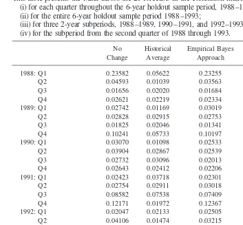
The performance of these five models is evaluated on the basis of minimizing the Mean Squared Error (MSE) across the set of 21 forecasts every quarter. Each model is applied to forecast correlations estimated on both a US Dollar basis and a home currency basis. Tables 6 and 7 present the MSE across all 21 forecasts in the correlation structure for each quarter of the 6-year holdout period, as well as for this entire 6-year period and three 2-year subperiods. In addition, due to the influence of the October 1987 international crash on the forecasts for the first quarter of 1988, we provide results for the subperiod covering the second quarter of 1988 through 1993.
Results for the first quarter of 1988 reveal that, while the forecast performance of the historical average model and ARIMA model is not greatly affected by the October 1987 crash, the same cannot be said for the remaining three models. This result is not surprising, as both the no-change and the empirical Bayes models rely on the previous quarter’s correlation matrix to forecast the current quarter’s matrix. Similarly, the economic model forecast is also heavily influenced by the value of world market volatility in the previous quarter. This behavior leads to forecasts from these three models that dramatically over-estimate the correlation matrix for the first quarter of 1988. In contrast, the historical average model and ARIMA model are not as greatly affected by the aberrant behavior during the fourth quarter of 1987, as this quarter’s correlation matrix makes up only a
18The exponentially weighted model employed in J. P. Morgan’sRiskMetrics(1996) package to forecast
variances and covariances is a special case of the general class of ARIMA models. Our application of this approach fits the unique ARIMA model that is appropriate for each pairwise time series of correlations and employs it to forecast. Details on the fitted ARIMA models employed in this application, along with their diagnostics, are available upon request.
portion of the information set employed by these two models to forecast the first quarter of 1988.
The aberrant behavior of the forecasts for the first quarter of 1988 leads us to focus on the forecasting results for the subperiod from the second quarter of 1988 through 1993, presented in the last row of Tables 6 and 7. Over this subperiod, the weakest forecast Table 6. Mean Squared Errors for Forecasts: US Dollar-Based Data
Five models are used to generate forecasts of the correlation matrix for next quarter, as follows: (1) The No Change model employs the correlation from the previous quarter as the forecast; (2) The Historical Average model uses the average correlation over the previous eight quarters; (3) The Empirical Bayes approach regresses each bilateral correlation toward the global mean
across all correlations of the previous quarter; (4) The ARIMA model is used to forecast 1-step-ahead;
(5) The fitted values from the economic model are used to project 1-step-ahead;
The estimation period for models (4) & (5) is 1972–1987; the holdout forecast period is 1988 –1993. By updating data and re-estimating models (4) & (5) each quarter over the 6-year holdout sample, we generate a set of 24 one-step-ahead forecasts of the correlation matrix for each model.
This table presents the MSE across the 21 forecasts in the correlation matrix: (i) for each quarter throughout the 6-year holdout sample period, 1988 –1993; (ii) for the entire 6-year holdout sample period 1988 –1993;
(iii) for three 2-year subperiods, 1988 –1989, 1990 –1991, and 1992–1993; and (iv) for the subperiod from the second quarter of 1988 through 1993.
No
1988: Q1 0.23582 0.05622 0.23255 0.05966 0.34584
Q2 0.04593 0.01039 0.03563 0.01523 0.01705
Q3 0.01656 0.02020 0.01684 0.01275 0.01520
Q4 0.02621 0.02219 0.02334 0.01590 0.02274
1989: Q1 0.02742 0.01169 0.03019 0.01845 0.01234
Q2 0.02828 0.02915 0.02753 0.02540 0.02960
Q3 0.01825 0.02046 0.01341 0.02479 0.02258
Q4 0.10241 0.05733 0.10197 0.06236 0.05325
1990: Q1 0.03070 0.01098 0.02533 0.01093 0.01358
Q2 0.03904 0.02867 0.02539 0.02031 0.02637
Q3 0.02732 0.03096 0.02013 0.03326 0.02371
Q4 0.02643 0.02412 0.02206 0.01970 0.01950
1991: Q1 0.02423 0.03718 0.02301 0.04201 0.01917
Q2 0.02754 0.02911 0.03018 0.02598 0.03092
Q3 0.08582 0.07538 0.07409 0.08491 0.05707
Q4 0.12171 0.01972 0.12367 0.03298 0.03729
1992: Q1 0.02047 0.02133 0.02505 0.02366 0.01518
Q2 0.04106 0.01474 0.03215 0.01751 0.02139
Q3 0.09475 0.07905 0.09166 0.04455 0.09985
Q4 0.05275 0.04678 0.03858 0.01891 0.02324
1993: Q1 0.02023 0.04538 0.01818 0.03098 0.02411
Q2 0.05255 0.05408 0.04891 0.04602 0.03560
Q3 0.03758 0.04817 0.03152 0.03565 0.05326
Q4 0.03979 0.01312 0.03195 0.01456 0.01693
Avg MSE 1988–1989 0.06261 0.02845 0.06018 0.02932 0.06482
Avg MSE 1990–1991 0.04785 0.03201 0.04298 0.03376 0.02845
Avg MSE 1992–1993 0.04490 0.04033 0.03975 0.02898 0.03620
Avg MSE 1988–1993 0.05179 0.03360 0.04764 0.03069 0.04316
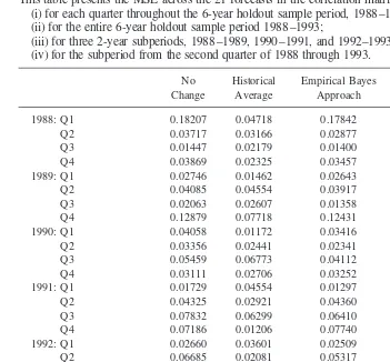
performance in terms of MSE is given by the naive model of no change from the previous quarter, for both US dollar and home currency returns. The empirical Bayes approach does not fare much better, ranking as the fourth best model for US dollar returns and the third best model for home currency returns. The ARIMA model performs well for US dollar Table 7. Mean Squared Errors for Forecasts: Home Currency Data
Five models are used to generate forecasts of the correlation matrix for next quarter, as follows: (1) The No Change model employs the correlation from the previous quarter as the forecast; (2) The Historical Average model uses the average correlation over the previous eight quarters; (3) The Empirical Bayes approach regresses each bilateral correlation toward the global mean
across all correlations of the previous quarter; (4) The ARIMA model is used to forecast 1-step-ahead;
(5) The fitted values from the economic model are used to project 1-step-ahead;
The estimation period for models (4) & (5) is 1972–1987; the holdout forecast period is 1988 –1993. By updating data and re-estimating models (4) & (5) each quarter over the 6-year holdout sample, we generate a set of 24 one-step-ahead forecasts of the correlation matrix for each model.
This table presents the MSE across the 21 forecasts in the correlation matrix: (i) for each quarter throughout the 6-year holdout sample period, 1988 –1993; (ii) for the entire 6-year holdout sample period 1988 –1993;
(iii) for three 2-year subperiods, 1988 –1989, 1990 –1991, and 1992–1993; and (iv) for the subperiod from the second quarter of 1988 through 1993.
No
1988: Q1 0.18207 0.04718 0.17842 0.05782 0.14023
Q2 0.03717 0.03166 0.02877 0.07376 0.05535
Q3 0.01447 0.02179 0.01400 0.04268 0.02686
Q4 0.03869 0.02325 0.03457 0.02115 0.02596
1989: Q1 0.02746 0.01462 0.02643 0.02236 0.01900
Q2 0.04085 0.04554 0.03917 0.04323 0.02241
Q3 0.02063 0.02607 0.01358 0.01493 0.01664
Q4 0.12879 0.07718 0.12431 0.08159 0.09777
1990: Q1 0.04058 0.01172 0.03416 0.02967 0.02957
Q2 0.03356 0.02441 0.02341 0.04069 0.01615
Q3 0.05459 0.06773 0.04112 0.08063 0.05529
Q4 0.03111 0.02706 0.03252 0.04661 0.01734
1991: Q1 0.01729 0.04554 0.01297 0.07746 0.03167
Q2 0.04325 0.02921 0.04360 0.04297 0.03477
Q3 0.07832 0.06299 0.06410 0.12861 0.07363
Q4 0.07186 0.01206 0.07740 0.01590 0.01796
1992: Q1 0.02660 0.03601 0.02509 0.01858 0.01979
Q2 0.06685 0.02081 0.05317 0.03585 0.04029
Q3 0.04976 0.02867 0.03596 0.02324 0.02587
Q4 0.04929 0.04835 0.04821 0.02709 0.02726
1993: Q1 0.02118 0.06143 0.01728 0.03878 0.02317
Q2 0.03718 0.09656 0.02644 0.05821 0.03868
Q3 0.04247 0.04261 0.03431 0.03072 0.03205
Q4 0.05033 0.01918 0.04074 0.02017 0.02869
Avg MSE 1988–1989 0.06127 0.03591 0.05741 0.04469 0.05053
Avg MSE 1990–1991 0.04632 0.03509 0.04116 0.05782 0.03455
Avg MSE 1992–1993 0.04296 0.04420 0.03515 0.03158 0.02948
Avg MSE 1988–1993 0.05018 0.03840 0.04457 0.04470 0.03818
returns (ranking first), but does considerably worse (fourth) for returns on a home currency basis. This outcome suggests that time series regularities may be more stable and predictable for correlations across exchange rates than across equity index returns. The historical average over the previous eight quarters consistently offers reasonably accurate forecasts that are worthy of note, ranking third for US dollar returns and second for home currency returns. Finally, the economic model performs well under both US dollar returns (ranking a close second) and home currency returns (ranking first). While these results are not necessarily overwhelming, the economic model does dominate in its ability to forecast during this holdout period. Similar results over the shorter 2-year holdout samples solidify the relative dominance of the economic model, especially for home currency forecasts.
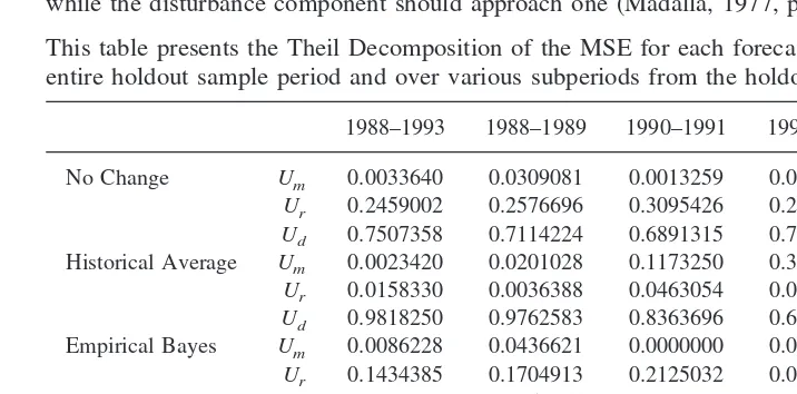
After documenting that the economic model dominates the other forecasting models in consistently minimizing MSE, we can gain additional insight into the forecast perfor-mance of each model by conducting a Theil decomposition of the MSE (Madalla, 1977). The Theil decomposition partitions the MSE into three components which sum to one: bias (Um), regression (Ur), and disturbance (Ud). Besides displaying a forecast profile with
the minimum MSE, the optimal forecasting model should ideally yield values ofUmand Ur that approach zero while Ud approaches one. Such a forecast profile would typify
forecast errors that fluctuate randomly about zero, and thus display little tendency for the model to systematically over- or under-estimate the actual values.
These Theil decompositions are presented in Tables 8 and 9 for US dollar returns and home currency returns, respectively. Again we focus on the forecast period covering the holdout sample that excludes the first quarter of 1988, presented in the last column of Table 8. Theil Decomposition of Forecast MSE: US Dollar-Based Data
The Theil Decomposition partitions the MSE of a set of forecasts into 3 additive components: (i)Um5bias component;
(ii)Ur5regression component; and (iii)Ud5disturbance component.
For the optimal forecasting model, the bias and regression components should approach zero while the disturbance component should approach one (Madalla, 1977, pp. 343–345).
This table presents the Theil Decomposition of the MSE for each forecasting model, over the entire holdout sample period and over various subperiods from the holdout sample.
1988–1993 1988–1989 1990–1991 1992–1993 1988Q2–1993
No Change Um 0.0033640 0.0309081 0.0013259 0.0002840 0.0000814
Ur 0.2459002 0.2576696 0.3095426 0.2124636 0.2119127
Ud 0.7507358 0.7114224 0.6891315 0.7872524 0.7880059
Historical Average Um 0.0023420 0.0201028 0.1173250 0.3099923 0.0024740
Ur 0.0158330 0.0036388 0.0463054 0.0057332 0.0187329
Ud 0.9818250 0.9762583 0.8363696 0.6842745 0.9787931
Empirical Bayes Um 0.0086228 0.0436621 0.0000000 0.0022806 0.0006563
Ur 0.1434385 0.1704913 0.2125032 0.0802900 0.0996870
Ud 0.8479386 0.7858466 0.7874968 0.9174294 0.8996567
ARIMA Model Um 0.0127502 0.0060997 0.1749821 0.0329274 0.0181984
Ur 0.0111766 0.0000253 0.0489162 0.0241418 0.0119014
Ud 0.9760732 0.9938750 0.7761018 0.9429309 0.9699002
Economic Model Um 0.0265206 0.0124100 0.0005429 0.1322994 0.0048421
Ur 0.1225076 0.2622355 0.0764341 0.0555171 0.0391367
Tables 8 and 9. Table 8 indicates that for US dollar returns the economic, historical average, and ARIMA models offer similarly desirable forecast profiles in terms of their Theil decomposition. However, the performance of the ARIMA model drops somewhat for home currency returns in Table 9, leaving the economic and historical average models as the dominant performers in terms of Theil decomposition.
V. Summary and Conclusions
Previous studies yield mixed evidence regarding the stability of the correlation structure across international equity markets. We employ daily data on national stock returns since 1972 to generate a quarterly time series in the correlation matrix. Stability tests on this time series overwhelmingly indicate that the correlation matrix changes substantively across both short and long time intervals, throughout the sample period 1972–1993. This outcome focuses attention on the issue of how and why the correlation structure changes over time.
A theoretical model specifying potential economic determinants of the correlation structure is proposed and estimated, using both US dollar denominated returns and home-currency returns. Results indicate the following behavior. For both US dollar returns and home-currency returns:
(1) world market volatility (WLDVOLij) is positively associated withrij; Table 9. Theil Decomposition of Forecast MSE: Home Currency Data
The Theil Decomposition partitions the MSE of a set of forecasts into 3 additive components: (i)Um5bias component;
(ii)Ur5regression component; and (iii)Ud5disturbance component.
For the optimal forecasting model, the bias and regression components should approach zero while the disturbance component should approach one (Madalla, 1977, pp. 343–345).
This table presents the Theil Decomposition of the MSE for each forecasting model, over the entire holdout sample period and over various subperiods from the holdout sample.
1988–1993 1988–1989 1990–1991 1992–1993 1988Q2–1993
No Change Um 0.0030100 0.0272836 0.0014379 0.0004003 0.0000055
Ur 0.2752795 0.2651327 0.3703286 0.2967222 0.2381793
Ud 0.7217105 0.7075837 0.6282335 0.7028775 0.7618152
Historical Average Um 0.0032052 0.0040444 0.2828797 0.3304780 0.0054201
Ur 0.0525208 0.0063974 0.0573262 0.0404575 0.0540870
Ud 0.9442740 0.9895583 0.6597941 0.6290645 0.9404929
Empirical Bayes Um 0.0080154 0.0402257 0.0000005 0.0022005 0.0009322
Ur 0.1614739 0.1756970 0.2633517 0.1233563 0.1140647
Ud 0.8305107 0.7840773 0.7366478 0.8744432 0.8850031
ARIMA Model Um 0.0948682 0.0749593 0.5119004 0.0378351 0.0892753
Ur 0.0543140 0.0184368 0.0422331 0.0741522 0.0583557
Ud 0.8508178 0.9066039 0.4458665 0.8880127 0.8523689
Economic Model Um 0.0044154 0.0012217 0.1685946 0.0693845 0.0219598
Ur 0.0955003 0.1768599 0.0883174 0.0615846 0.0452333
(2) a positive trend (TREND) in therijappears in the first half of this 22-year period,
from 1972 to 1982, while no trend appears from 1983 to 1993; and (3) exchange rate volatility (XRSDij) has a dampening effect onrij.
In addition, to a lesser extent, for US dollar returns:
(4) term structure differentials (LOSHi2 LOSHj) are negatively related torij;
and for home-currency returns:
(5) real interest differentials (INTi2INTj) are negatively related to rij; and
(6) the world market return is negatively associated withrij.
This analysis and evidence contributes to our understanding of the dynamics of global integration. For example, these results corroborate our theoretical expectations that divergent behavior across nations in several macroeconomic variables tends to be asso-ciated with divergent behavior across national equity markets, resulting in lower market correlations. In addition, it is noteworthy that the first and last factors listed above indicate an increase in comovement across international equity markets when world markets are more volatile and/or falling. This result implies a decline in the risk-reduction benefits of international diversification at the very time when these benefits are needed most (Erb et al., 1994, Solnik et al., 1996).
Finally, we employ the economic model to generate out-of-sample short-term forecasts of the correlation matrix. The forecast performance of this model is seen to dominate that of four alternative forecasting techniques that ignore economic determinants of the correlation structure. This evidence adds credence to the validity of the theoretical economic model, and suggests a potential opportunity for portfolio managers to improve upon their portfolio selection techniques.
On the other hand, while these results document an improvement in the ability to generate short term forecasts, the issue of longer term forecasting capabilities is unre-solved. As a result, the question of whether this economic-based forecasting model can be employed to generate “optimal” ex ante international portfolios with enhanced ex post performance remains for future inquiry.
We gratefully acknowledge support from University of Kansas GRF Grant #3710. We also wish to acknowledge the helpful comments of William Beedles, Ken Cogger, Ali Fatemi, Peter Gillett, O. Maurice Joy, George Pinches, J. Jay Choi, and two anonymous referees. Morgan Stanley provided the data. These do not necessarily reflect the views of Morgan Stanley. Please do not quote without permission.
References
Arshanapalli, B., and Doukas, J. 1993. International stock market linkages: Evidence from the pre-and post-October 1987 period.Journal of Banking and Finance17:193–208.
Bachman, D., Choi, J. J., Jeon, B. N., and Kopecky, K. 1996. Common factors in international stock prices: Evidence from a cointegration study.International Review of Financial Analysis5(1): 39–53.