www.elsevier.nlrlocatereconbase
Illicit drug use, unemployment, and
occupational attainment
Ziggy MacDonald
), Stephen Pudney
Public Sector Economics Research Centre, Department of Economics, UniÕersity of Leicester,
UniÕersity Road, Leicester LE1 7RH, UK
Received 11 November 1998; received in revised form 28 March 2000; accepted 10 May 2000
Abstract
Ž .
In this paper, we use data from the British Crime Survey BCS to examine the effect of illicit drug use on labour market outcomes. We find very little evidence to support any relationship between drug use, hard or soft, and occupational attainment. However, we find compelling evidence to suggest that drug use, particularly the use of opiates, cocaine and crack cocaine, is associated with an increased risk of unemployment, regardless of age or gender.q2000 Elsevier Science B.V. All rights reserved.
JEL classification: C51; I12; J24
Keywords: Illicit drugs; Labour market participation; Occupational attainment
1. Introduction
Substance abuse is widely considered to be one of society’s ills, for its private and social impacts on health and criminal activity. There is, however, a growing area of research into the relationship between substance abuse and labour market outcomes. The impact of alcohol consumption on earnings has received particular attention in recent years, but there is also concern about the effects of illicit drug
Ž .
use on labour market outcomes, an issue originally highlighted by Culyer 1973 . The negative consequences of drug use for the physical and psychological well
)Corresponding author. Tel.:q44-116-252-2894; fax:q44-116-252-2908.
Ž .
E-mail address: [email protected] Z. MacDonald .
0167-6296r00r$ - see front matterq2000 Elsevier Science B.V. All rights reserved.
Ž .
being of individuals can lead to chronic absenteeism and frequent spells out of the labour market. This reduced labour market experience of drug users will ultimately result in a lower aggregate level of human capital accumulation, tending to reduce
Ž .
overall productivity and hence, living standards Kaestner, 1994a . Thus, assuming that workers receive the value of their marginal product as pay, then the reduced productivity level of drug users would manifest itself through lower wages. Moreover, psychological or physical dependence implies that these impacts are not simply an optimal private decision in the long term.
Although the negative relationship between illicit drug use and productivity seems plausible, there has been recent work questioning this view. Modern research recognises that single-equation models suffer from bias arising from the simultaneity of drug use and wages, and from the existence of unobserved heterogeneity. These bring into question the direction of causality in a wage equation which has a measure of drug use as an explanatory variable. The endogeneity issue is clear if we think of drugs as a normal consumption good, the level of which is determined in response to market wages and non-labour income. If, however, we also assume that drug use has a negative impact on an individual’s wage, then this implies simultaneous causation between drug use and wages. The heterogeneity problem arises because unobserved attributes that affect wages or employment outcomes are quite likely to overlap with the characteristics that influence an individual’s choice to take drugs. For example, the unobserved characteristic could be a high rate of time preference, causing individuals to select high-paying jobs without consideration for investment in human capital, but also,
Ž .
according to Becker and Murphy 1988 , making them more likely to take drugs. The purpose of this paper is to address these issues that have been raised in a US context, using data from the UK. To do this, we use data from the British
Ž .
Crime Survey BCS and estimate a joint model covering past and current drug use together with unemployment and occupational attainment. The BCS sample spans a greater age range than previously used US data, so we are also able to
Ž .
consider the lifespan perspective of illicit drug use Kandel et al., 1995 . In Section 2, we discuss the relevant literature in this area, including that which focuses on the impact of alcohol abuse on labour market outcomes. We then consider the BCS data set, its advantages and shortcomings, and the sample properties. In Section 4, we develop our empirical model and present our estimation results in Section 5.
2. Past research
those in work. Against this background, there is also some debate over the issue of endogeneity and whether it really is a problem when estimating the effect of substance abuse on labour market outcomes. Overall, as we shall see, the results presented in the literature are far from unequivocal.
2.1. Drug use and labour supply
The relationship between substance abuse and labour supply tends not to generate any consensus in the literature. For example, although most economists would argue that substance abuse will impact on labour supply, perhaps through some detrimental effect on health, there are some who argue that it is
unemploy-Ž .
ment that tends to foster drug use, rather than the reverse Peck and Plant, 1987 . Where there is agreement over the likely direction of causality, there is a mixture of results that leaves the impact of substance use on labour supply open to question. For example, in considering alcohol abuse and labour supply, Mullahy
Ž .
and Sindelar 1991, 1996 find a statistically significant negative association
Ž . Ž
between these variables, whereas Kenkel and Ribar 1994 do not although they find a small statistically significant negative association between heavy drinking
.
and the labour supply of males . The different conclusions that are drawn from these studies may relate to the different definitions of labour supply that are used. Kenkel and Ribar focus on the hours of labour supplied, whereas both the Mullahy
Ž .
and Sindelar papers focus on participation. However, Kaestner 1994a , using the Ž
same data set as Kenkel and Ribar the US National Longitudinal Survey of
. Ž .
Youth, NLSY , finds a negative association between marijuana cannabis or cocaine use and the hours of labour supplied by young males.
All these studies deal with the issue of endogeneity of substance abuse and wages in standard ways, yet there appears to be a lack of consensus in the results.
Ž .
Against this, Zarkin et al. 1998a suggest that substance abuse and hours worked are not endogenously determined. Following extensive tests for exogeneity of substance abuse variables, they estimate a single-equation model of labour supply for a sample of 18–24-year-old men taken from the US National Household Survey on Drug Abuse. They find no significant relationship between past month labour supply and the use of cigarettes, alcohol or cocaine in the past month. Although they find a significant positive association with past month cannabis use, they conclude that there is little evidence to support a robust labour supply–drug
Ž .
use relationship. Similarly, although the cross-sectional results of Kaestner 1994a support a negative relationship between drug use and hours of labour supplied, his longitudinal estimates do not support any systematic effect of drug use on labour supply.
2.2. Drug use and attainment
significant negative relationship between substance abuse and wages. Kaestner Ž1991 , using data from the NLSY, finds that, if anything, increased frequency of.
Ž .
illicit drug use in this case, cocaine or marijuana is associated with higher wages. This result, consistent across gender and age groups, was found using a Heckman
Ž .
two-stage estimate of a wage equation. Likewise, Gill and Michaels 1992 and
Ž .
Register and Williams 1992 , using the same data as Kaestner but slightly different approaches to control for the self-selection of individuals into drug use and the labour market, find very similar results. These findings echo the results that have been found for the relationship between alcohol and wages. For example,
Ž .
Berger and Leigh 1988 , using data from the US Quality of Employment Survey and taking account of self-selection, found that drinkers receive higher wages, on average, compared to non-drinkers. More recent work has recognised a non-linear relationship between alcohol consumption and wages. For example, using different
Ž . Ž .
sources of data, French and Zarkin 1995 , Heien 1996 , Hamilton and Hamilton Ž1997 and MacDonald and Shields 2000 present results that support a quadratic. Ž . relationship between drinking intensity and wages.1 In each case, alcohol con-sumption is shown to have an increasingly positive association with wages up to a point, after which there is a rapid drop-off in earnings for heavy drinkers compared to moderate drinkers.
There is, however, some research that questions this general view. As a
Ž .
follow-up to previous results, Kaestner 1994b presents cross-sectional and longitudinal estimates using two waves of the NLSY. The cross-sectional results are generally consistent with the previous studies, but the longitudinal estimates only provide partial support for the positive relationship between drug use and wages. The results suggest that the wage–drug use relationship varies according to the type of drug and individual; e.g., a positive relationship between cocaine use and wages for females, but a negative relationship between marijuana use and
Ž .
wages for males. Moreover, Kandel et al. 1995 suggest that the relationship between drug use and wages will vary with the stage of an individual’s career. Using a follow-up cohort of the NLSY, they find a positive relationship between drug use and wages in the early stages of an individual’s career, but a negative
Ž .
relationship later on in the career in the mid-thirties . However, Burgess and
Ž .
Propper 1998 , using the same data source, are not able to replicate this finding. Ž
In their analysis, they consider the effects of early life behaviour such as drug and .
alcohol consumption and later life outcomes, including productivity. Their results suggest that adolescent alcohol and soft drug use have little or no effect on the earnings of men in their late twenties or thirties, although they do find that early hard drug use has a significant negative impact.
1 Ž .
3. Data and sample
It is quite clear from the literature that the majority of research into the relationship between illicit drug use and labour market outcomes has used the US
Ž .
Longitudinal Survey of Youth NLSY . Researchers in the US are fortunate to have several different sources of drug misuse information. In contrast, the UK undertakes very little monitoring of drug use at a national level. Apart from
Ž
official sources of information such as the Home Office ‘Addicts Index’ — now .
closed , and the occasional local survey, the only other major source of compara-ble drug misuse information in the UK is the BCS. The BCS is a household victimisation survey, representative of the adult population of England and Wales.2 Face-to-face interviews are carried out by the staff of the Social and Community Planning Research in the first few months of the survey year, and they cover individuals’ experiences of crime and crime-related issues for the 12–14 months preceding the interview. Information on drug misuse has been collected in the 1992, 1994, 1996 and 1998 sweeps of the BCS, although the 1992 survey is not
Ž .
suitable for comparison with later surveys Ramsay and Percy, 1997 and that of 1998 is not in the public domain. In this analysis, we pool the 1994 and 1996 data, which after losses for incomplete records and exclusion of those aged over 50, leave us with a sample of 13,908 individuals with complete drug use information Ž6404 for 1994 and 7504 for 1996 ..
3.1. Self-reported data
Before we present our analysis of the BCS drug use information, we should first consider the reliability of these data. The BCS drug use information is self-reported, which is the norm for this type of analysis. The difficulties associ-ated with self-reported data are widely recognised, particularly when the subject
Ž .
matter is sensitive. Indeed, Hoyt and Chaloupka 1994 concluded that previous research that has used the NLSY is particularly vulnerable to the large reporting errors that accompany the substance use measures. Typically, we expect some form of underreporting from questions about drug use, and this is likely to vary between socio-economic groups. For example, in an analysis of the NLSY,
Ž .
Mensch and Kandel 1988 found that, compared to individuals with a relatively heavy use of drugs, light users tend to underreport their consumption, as do females and ethnic minorities. In support of this last point, Fendrich and Vaughn Ž1994 found that the impact of ethnicity on underreporting of substance abuse is a.
2 Ž .
For more details of the sampling procedure for the 1994 survey, see White and Malbon 1995 , and
Ž .
particularly important factor. There is also evidence to link survey conditions to
Ž .
individual reporting behaviour. Hoyt and Chaloupka 1994 find that the presence of others during the administration of the survey, the use of telephone interviews and self-administration of the survey can all lead to misreporting. Moreover,
Ž .
O’Muircheartaigh and Campanelli 1998 report that the interviewer can be the biggest source of error in survey data.
In common with all other studies, there is very little we can do to overcome some of the potential sources of error. However, one thing in our favour is the method used to collect the BCS drug use information. The BCS self-completion questionnaire is administered using a laptop computer, which is passed over to the interviewee following some brief instructions from the interviewer. This method of eliciting information may have some advantages over traditional techniques, not least because it offers the same level of anonymity as sealed booklet methods ŽMcAllister and Makkai, 1991 . Indeed, it is claimed that the change to computers. for self-reporting in the BCS resulted in the identification of some groups of users Žsuch as heroin users from the Asian community that had previously not reported.
Ž .
any drug consumption Ramsay and Percy, 1997 . Overall, given the typical survey design, any drug use data collected via surveys are likely to miss certain high-risk groups and be subject to a variety of sources of error. We recognise this as a problem, but take some comfort from the data collection method used in the BCS.
3.2. Drug use information
Using a laptop computer, BCS interviewees aged 16–59 are required to answer Ž
questions about their experience of 14 commonly abused drugs including a bogus .
drug Semeron, put in the survey to test for false claiming . Survey respondents are asked whether they have ever taken any of the listed drugs, taken any in the past
Ž
12 months or in the past month. In a previous analysis MacDonald and Pudney, .
2000 , we separated drug use into a ‘hard’ and a ‘soft’ category, according to their classification in the Misuse of Drugs Act 1971, and reflecting the common perception of differing risk between drugs. In this analysis, and following Ramsay
Ž .
and Spiller 1997 , we also consider an alternative grouping of the BCS drugs that reflects the context in which they are likely to be consumed. Our first group is composed of the so-called ‘recreational’ drugs. These include the ‘dance drugs’ Žamphetamines, amyl nitrite ‘poppers’ , ecstasy, LSD, and magic mushrooms ,Ž . . which are synonymous with ‘clubbing’, and cannabis, which is by far the most common drug to be consumed. We have labeled our second group as ‘dependency
Ž .
In particular, whereas ecstasy, LSD and magic mushrooms are regarded as class A Žhard drugs in the Misuse of Drugs Act, in this alternative grouping, we move. them into the recreational group, leaving a much smaller set of drugs in the more dangerous dependency group.
In Table 1, we summarise the frequency of reported use of these drugs by men Ž and women for two age cohorts: those aged 16–25, and those aged 26–50 we
. exclude those over 50 as this group has negligible rates of reported drug use . The splitting of the sample reflects a common finding in the literature which suggests that individuals tend to ‘mature out’ of drug use in their late twenties or early
Ž
thirties Gill and Michaels, 1991; Labouvie, 1996; Ramsay and Percy, 1996; .
MacDonald, 1999 . Thus, we would expect drug use to be more prevalent in the youngest group. There is also a likely cohort effect, stemming from the increasing
Ž .
prevalence of the youth drug ‘culture’ over time Parker and Measham, 1994 . We restrict the presentation of results in Table 1 to just the recreational and depen-dency drugs, although similar results are found for the hard and soft drug groups. The figures in Table 1 reveal that the use of recreational drugs is far more prevalent than dependency drugs for both age cohorts, but there is a clear pattern
Ž .
of diminishing use both ever and recent from the younger to the older group and from males to females. In particular, the figures suggest that almost half of the young men in the sample have tried a recreational drug at some point in their life, whereas the figure reduces to a third for the older group. Moreover, for both men and women, the proportion of the older group reporting any use ever is almost the same as the proportion of the younger group who report recent use. In terms of the gender divide, it is quite clear that men have a much higher rate of reported drug use than do women, but the age difference is still important. For example, about one in five young women reports recent use of recreational drugs, whereas the rate
Table 1
Ž .
Past and present illicit drug use %
Age 16–25 Age 26–50
Men Women Men Women
Recreational drugs
Ž . Ž . Ž . Ž .
Ever used 47.26 1.41 35.10 1.35 31.47 0.60 20.03 0.55
Ž . Ž . Ž . Ž .
Only used in past 16.52 1.05 15.87 1.03 21.98 0.53 14.65 0.48
Ž . Ž . Ž . Ž .
Recently used 30.74 1.30 19.20 1.11 9.49 0.38 5.38 0.31
Dependency drugs
Ž . Ž . Ž . Ž .
Ever used 6.20 0.68 3.27 0.50 4.21 0.26 2.48 0.21
Ž . Ž . Ž . Ž .
Only used in past 3.49 0.52 2.23 0.42 3.10 0.22 1.94 0.19
Ž . Ž . Ž . Ž .
Recently used 2.70 0.46 1.04 0.29 1.11 0.13 0.54 0.10
Observations 1259 1255 6037 5357
is less than one in 20 for older women.3 We also observe that for younger men and women, a much greater proportion report recent use of recreational drugs than use only in the past. This observation is reversed for the older group, where the rate of use in the past only is more than double the rate of recent use.
3.3. Labour market information
As we highlighted in the review of literature, there are two dimensions to the impact of drug use on labour market outcomes. The first we consider is the impact
Ž .
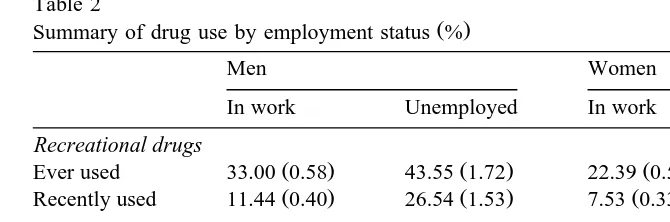
of drug use on the risk of unemployment. Kaestner 1994a and Zarkin et al. Ž1998b consider the drug use–employment relationship by focusing on labour. supply as measured by the number of hours worked. In this analysis, we focus on employment status rather than hours worked. In Table 2, we summarise drug use according to employment status for respondents aged from 16 to 50. BCS respondents are classified as employed if they confirm that they were in paid
Ž .
employment or self-employment in the previous week full time or part time . Our unemployed category covers all those who were not employed, but reported that they were currently looking for work. Thus, we exclude individuals in full-time education, those who are sick or disabled, retired or looking after the homerfamily. Table 2 reveals a sharp contrast in the reported drug use rates between the employed and the unemployed. In all cases, there appears to be a much higher prevalence of drug use among the unemployed group. This is in sharp contrast to the data from the NLSY, where there is no significant differential between the
Ž
level of drug use of those in work and those who are unemployed Kaestner, .
1994a . In the current sample, the proportion of unemployed men reporting recent use of dependency drugs is higher than the proportion of the employed men reporting any use ever.
The second dimension to the impact of drug use on labour market outcomes is the relationship between drug use and occupational attainment for those who are in work. In the literature, the majority of research into the relationship between substance abuse and productivity have made use of individual data on earnings. Unfortunately, individual wages are not observed in the BCS. The survey provides
Ž .
detail of total household income coded in bands , but it is unlikely that household income is relevant for individual drug use: an individual with a well-off parent but no personal income may still be involved in drugs. As an alternative, we focus on occupational success. As it is difficult to define and rank occupations objectively,
Ž .
we use an approach due to Nickell 1982 and recently used by Harper and Haq Ž1997 and MacDonald and Shields 2000 . Here we rank occupations using the. Ž . average earnings associated with an individual’s occupation. In other words, we define occupational success in terms of relative levels of average hourly pay for
3
Table 2
Ž .
Summary of drug use by employment status %
Men Women
In work Unemployed In work Unemployed
Recreational drugs
Ž . Ž . Ž . Ž .
Ever used 33.00 0.58 43.55 1.72 22.39 0.53 30.56 2.32
Ž . Ž . Ž . Ž .
Recently used 11.44 0.40 26.54 1.53 7.53 0.33 15.40 1.82
Dependency drugs
Ž . Ž . Ž . Ž .
Ever used 3.88 0.24 9.77 1.03 2.49 0.20 4.80 1.08
Ž . Ž . Ž . Ž .
Recently used 1.01 0.12 4.34 0.71 0.60 0.10 1.51 0.61
Observations 6467 829 6216 577
Standard errors in parentheses.
the occupation in question. It is thus to be interpreted as a measure of the labour market status of the individual’s occupation, rather than as an indicator of his or her actual wages, or of success within an occupation. We return to this issue in Section 5 when interpreting the results.
We calculate the mean hourly wage associated with each occupation using
Ž .
pooled data from the UK Quarterly Labour Force Survey QLFS for 1993, 1994
Ž .
and 1995 12 quarterly surveys in all . The QLFS codes occupation to the three-digit level of the Standard Occupational Classification, which gives 899 possible occupation categories. These occupational codes are also used in the BCS, allowing us to map the mean hourly wage from each occupational category in the QLFS to individual occupations in the BCS. Given that there are nearly 900 occupations defined in the survey, we treat the associated mean hourly wage as a continuous variable in our analysis.
A casual look at the distribution of occupational status by drug use status reveals an interesting feature in the current sample, which reflects findings from other data. Average occupational status for those who have ever used drugs is higher than the wage for those who report no drug use ever. This result holds for men and women, for the younger and older cohorts, and for any category of drug use. This last observation suggests two potentially opposing outcomes of drug use: unemployment or enhanced occupational attainment. These two associations may represent opposite causal links: drug use may raise the risk of unemployment,
Ž .
whereas occupational success and high income may raise the demand for drugs. We consider these outcomes further in the following sections, focusing on the difference between past and current drug use.
4. The empirical model
12 months preceding the interview.4 These two periods allow us to define past and current drug use. The levels of drug use in these two periods are represented by a
Ž .
pair of trichotomous indicators dt ts1,2 , where dts0 indicates no drug use,
dts1 indicates use the use of ‘soft’ drugs only and dts2 indicates the use of
Ž .
‘hard’ or hard and soft drugs. We present results below for two alternative definitions of ‘soft’ and ‘hard’ drugs. We also define two indicators of labour market outcomes: current unemployment u and, for those in work, occupational attainment a. Both relate only to the current period. The variable u is a binary indicator, and the occupational attainment variable a is treated as continuous.
Before we can define our empirical model, we first have to confront a serious observational problem stemming from the design of the questionnaire used in the
Ž .
BCS and in other US and European surveys . The respondent is asked only whether or not hershe has ever used drugs, and, if so, whether or not within the last year. This questionnaire structure has the unfortunate feature that if a respondent reports drug use in the current period, we do not know whether or not there was any use in the past period. Thus, d1 and d2 are only partially observable. Nevertheless, it is possible to estimate a suitable model by means of an iterative maximum likelihood method.
First, consider the determination of past drug use. We define a latent variable
d) which represents an individual’s past propensity to consume drugs. This drives
1
the observed indicator of actual drug use, d , through an ordered probit mecha-1 nism:
d)sx b q´ ,
Ž .
11 1 1 1
d srF
Ž
C Fd)-C.
, rs0,1,2,Ž .
21 1 r 1 1 rq1
Ž .
whereF J is the indicator function, equal to 1 if the event J occurs and 0 otherwise. C0s y`, C3s q`and C , C are unknown threshold parameters; x1 2 1 is a row vector of personal and demographic attributes, b1 is the corresponding
Ž .
vector of parameters, and ´1 is a N 0,1 random error.
The second stage of the model determines current drug use, current unemploy-ment and occupational attainunemploy-ment jointly, but conditional on past drug use. This is
Ž ) ) ).
achieved through a system of three latent variables d , u , and a2 representing the individual’s unobserved current propensities to consume drugs, to be
unem-4
ployed, and to do well when employed. These are generated by the following are the corresponding vectors of parameters, and ´2. . .´4 are errors with a trivariate normal distribution with zero means, unit variances and unrestricted
4
correlations, conditional on xs x , x , x1 2 3 and d . The variables1 j1 and j2 are
Ž .
binary indicators defined as jrsF d1sr . Thus, e.g., the total impact of ‘hard’
drug use on the tendency for unemployment is represented byd32.
The observable counterparts of these latent variables are the indicators of current drug use d , unemployment u and occupational achievement a. The latent2
Ž Ž . Ž ..
variables Eqs. 3 and 4 are assumed to generate the observed states by means of the following relationships:
d srF
Ž
C Fd)-C.
, rs0,1,2,Ž .
62 2 r 2 2 rq1
usF
Ž
u))0 ,.
Ž .
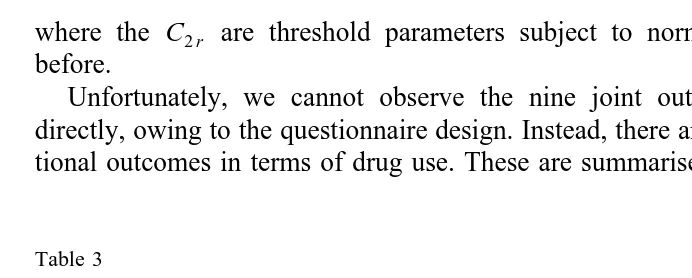
7where the C2 r are threshold parameters subject to normalising restrictions as before.
Unfortunately, we cannot observe the nine joint outcomes for d1 and d2 directly, owing to the questionnaire design. Instead, there are six possible observa-tional outcomes in terms of drug use. These are summarised in Table 3.
Table 3
Ž Ž . Ž ..
Given the linearrnormal structure Eqs. 1 – 7 , the outcome probabilities are
Ž . Ž
readily but very tediously constructed see MacDonald and Pudney, 2000 for
. Ž . 5
more details . They require evaluation of at most bivariate normal probabilities. These probabilities are then used to construct the following log-likelihood func-tion, which we maximised numerically using GAUSS MAXLIK software:
n
< <
ln Ls
Ý
lnPr dŽ
1 i x1 i.
qlnPr d ,u , a x , x , x , dŽ
2 i i i 2 i 3 i 4 i 1 i.
4
.Ž .
8is1
5. Results
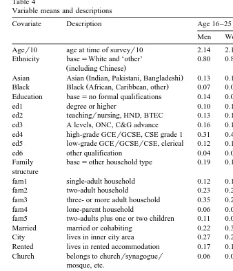
In our analysis, we provide separate estimates for our two age groups and for men and women. For a description of all the variables used in this analysis and their mean values, see Table 4. In each case, we present estimates for two models.
Ž .
The first model 1 reflects the drug use categories previously defined in Section 3 Žrecreational and dependency drugs . In the second model 2 , we focus on our. Ž . previous classification of drugs that is embedded in UK Law. Thus, we have a
Ž .
‘soft’ drug category class B or C consisting of amphetamines, cannabis and unprescribed tranquilisers; and a ‘hard’ drug category that includes cocaine, crack, heroin, unprescribed methadone, LSD, magic mushrooms and ecstasy. We begin by briefly discussing the results for the ordered probit estimates of past and current drug use.
5.1. Past and current drug use
Ž .
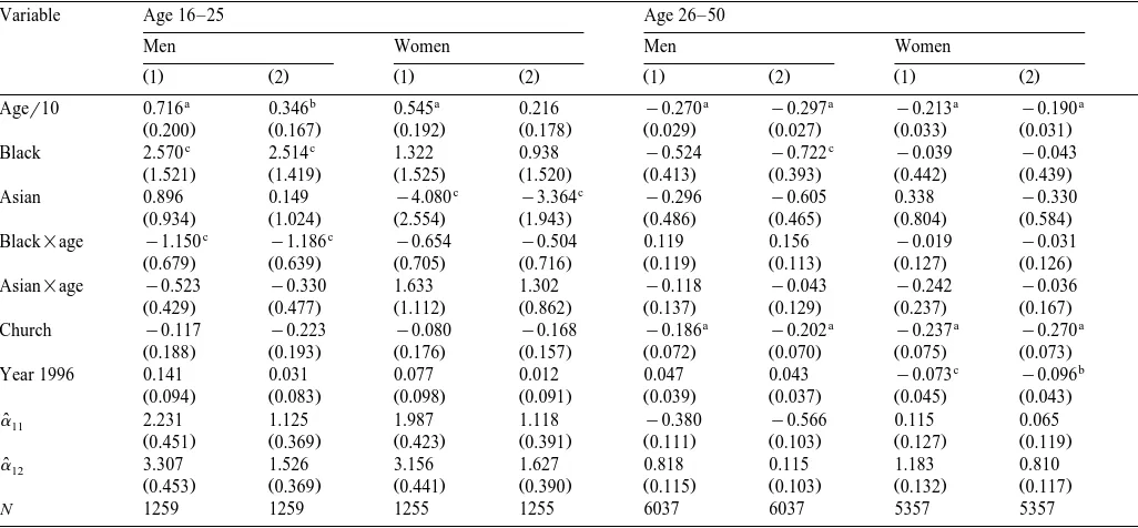
Following Sickles and Taubman 1991 , the past drug use component of models Ž . Ž .1 – 2 is specified relatively simply to include only basic demographic variables, plus religious practice and some simple age–race interactions.6 This choice of covariates reflects the need to include only exogenous factors that are unlikely to be affected by past drug use. The inclusion of religious practice does not strictly fall into this category, but it is likely that in most cases, religious orientation is formed at an age before experimentation with drugs typically begins. The current drug use component is also specified as a simple ordered probit, but with an expanded set of covariates describing the current demographic nature of the individual and hisrher household, current drinking habits, and also the lag effect
5 Ž .
Further details in the form of a GAUSS procedure are available upon request from the authors.
6
Table 4
Variable means and descriptions
Covariate Description Age 16–25 Age 26–50
Men Women Men Women
Ager10 age at time of surveyr10 2.14 2.15 3.71 3.71
Ethnicity basesWhite and ‘other’ 0.80 0.83 0.85 0.87
Žincluding Chinese.
Ž .
Asian Asian Indian, Pakistani, Bangladeshi 0.13 0.10 0.08 0.05
Ž .
Black Black African, Caribbean, other 0.07 0.07 0.07 0.09 Education basesno formal qualifications 0.14 0.09 0.18 0.19
ed1 degree or higher 0.10 0.11 0.20 0.16
ed2 teachingrnursing, HND, BTEC 0.13 0.11 0.17 0.13
ed3 A levels, ONC, C&G advance 0.16 0.17 0.12 0.10
ed4 high-grade GCErGCSE, CSE grade 1 0.31 0.40 0.20 0.28
ed5 low-grade GCErGCSErCSE, clerical 0.12 0.11 0.08 0.09
ed6 other qualification 0.04 0.03 0.05 0.04
Family basesother household type 0.19 0.17 0.16 0.13
structure
fam1 single-adult household 0.12 0.11 0.18 0.14
fam2 two-adult household 0.23 0.29 0.24 0.25
fam3 three- or more adult household 0.35 0.29 0.09 0.10
fam4 lone-parent household 0.06 0.09 0.09 0.17
fam5 two-adults plus one or two children 0.11 0.09 0.32 0.29
Married married or cohabiting 0.22 0.32 0.73 0.67
City lives in inner city area 0.27 0.27 0.23 0.23
Rented lives in rented accommodation 0.17 0.18 0.10 0.09
Church belongs to churchrsynagoguer 0.06 0.09 0.09 0.12
mosque, etc.
freqdrnk regular drinker 0.26 0.19 0.32 0.22
Year 1996 year dummy 0.51 0.52 0.54 0.55
Rec. ever ever used recreational drugs 0.47 0.35 0.31 0.20 Rec. recent recent use of recreational drugs 0.31 0.19 0.09 0.05
Dep. ever ever used dependency drugs 0.06 0.03 0.04 0.02
Dep. recent recent use of dependency drugs 0.03 0.01 0.01 0.01
Soft ever ever used soft drugs 0.44 0.33 0.31 0.22
Soft recent recent use of soft drugs 0.30 0.19 0.09 0.06
Hard ever ever used hard drugs 0.23 0.14 0.11 0.06
Hard recent recent use of hard drugs 0.10 0.05 0.02 0.01
Unemployed currently unemployed 0.19 0.11 0.10 0.05
Mn. hr. wage mean hourly occupational wage 6.04 5.60 7.34 6.36
of past drug use. The results for the past and current drug use components are summarised in Tables 5 and 6. In all cases, there is little difference between the
Ž . Ž . estimates for models 1 and 2 .
()
The probability of past drug use: ordered probit estimates
Variable Age 16–25 Age 26–50
Men Women Men Women
Ž .1 Ž .2 Ž .1 Ž .2 Ž .1 Ž .2 Ž .1 Ž .2
a b a a a a a
Ager10 0.716 0.346 0.545 0.216 y0.270 y0.297 y0.213 y0.190
Ž0.200. Ž0.167. Ž0.192. Ž0.178. Ž0.029. Ž0.027. Ž0.033. Ž0.031.
c c c
Black 2.570 2.514 1.322 0.938 y0.524 y0.722 y0.039 y0.043
Ž1.521. Ž1.419. Ž1.525. Ž1.520. Ž0.413. Ž0.393. Ž0.442. Ž0.439.
c c
Asian 0.896 0.149 y4.080 y3.364 y0.296 y0.605 0.338 y0.330
Ž0.934. Ž1.024. Ž2.554. Ž1.943. Ž0.486. Ž0.465. Ž0.804. Ž0.584.
c c
Black=age y1.150 y1.186 y0.654 y0.504 0.119 0.156 y0.019 y0.031
Ž0.679. Ž0.639. Ž0.705. Ž0.716. Ž0.119. Ž0.113. Ž0.127. Ž0.126.
Asian=age y0.523 y0.330 1.633 1.302 y0.118 y0.043 y0.242 y0.036
Ž0.429. Ž0.477. Ž1.112. Ž0.862. Ž0.137. Ž0.129. Ž0.237. Ž0.167.
a a a a
Church y0.117 y0.223 y0.080 y0.168 y0.186 y0.202 y0.237 y0.270
Ž0.188. Ž0.193. Ž0.176. Ž0.157. Ž0.072. Ž0.070. Ž0.075. Ž0.073.
c b
Year 1996 0.141 0.031 0.077 0.012 0.047 0.043 y0.073 y0.096
Ž0.094. Ž0.083. Ž0.098. Ž0.091. Ž0.039. Ž0.037. Ž0.045. Ž0.043.
aˆ11 2.231 1.125 1.987 1.118 y0.380 y0.566 0.115 0.065
Ž0.451. Ž0.369. Ž0.423. Ž0.391. Ž0.111. Ž0.103. Ž0.127. Ž0.119.
aˆ12 3.307 1.526 3.156 1.627 0.818 0.115 1.183 0.810
Ž0.453. Ž0.369. Ž0.441. Ž0.390. Ž0.115. Ž0.103. Ž0.132. Ž0.117.
N 1259 1259 1255 1255 6037 6037 5357 5357
period lengthens as we consider older cohorts. We find a significant negative association between age and past drug use for the older cohort, but for the younger cohort, the association is positive, although more noticeable for the first model. The positive association of drug use with age for the younger group presumably reflects the effect of the passage of time — older people have simply had more time in which to take drugs. The negative coefficient on age for the older cohort, however, probably reflects a cohort effect: that when those in the older cohort were of a typical drug-taking age, drug use was far less widespread.
Concentrating on our other variables, the impact of religious attendance appears particularly important for the older cohort, with a significant reduction in the probability of past drug use for those who report regular attendance at ChurchrMosquerSynagogue, etc. However, this association is not statistically significant for the younger cohort, although the sign on the coefficient is negative for all estimates. Where we observe ethnic differences, the interaction between ethnicity and age is quite complex. For example, for the younger male cohort, although being of a Black ethnic origin appears to be positively associated with past drug use, the interaction term with age suggests that this result is only true for the youngest of this cohort. We observe the same effect for Asians, but the estimated coefficients are not statistically significant. Finally, the results for the younger cohort also suggest that young Asian women are less likely to have consumed drugs in the past.
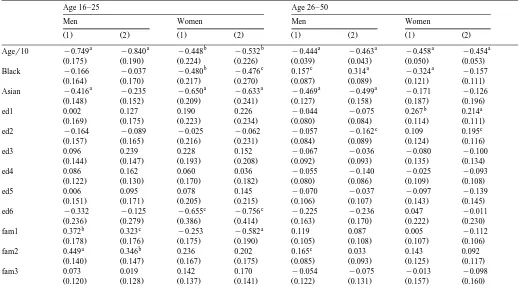
The results in Table 6 relate to drug use in the 12 months prior to the BCS interview. As with past drug use, age is an important factor; however, in all cases, there is a significant negative association between age and current drug use. We also find that in all cases, Asians are less likely than Whites to have consumed any drugs in the past year. Although this is mostly the case for individuals of Black origin, we do find that older Black men are more likely than Whites to have
Ž .
consumed drugs however defined in the past year. Other factors with statistically
Ž .
significant estimated coefficients include the impact of marriage yve , location
Ž . Ž .
in the inner city qve , living in rented accommodation qve and alcohol
Ž .
consumption qve . There is also evidence of marginal effects of religious
Ž . Ž
attendance yve for young men , living in all-adult households qve for young
. Ž .7
men, but negative for women , and being a lone parent qve for young women .
7
We note that there is some concern raised in the literature over the possible endogeneity of
Ž
education, family formation and marriage in substance abuse equations Burgess and Propper, 1998;
. Ž .
()
The probability of current drug use: ordered probit estimates
Age 16–25 Age 26–50
Men Women Men Women
Ž .1 Ž .2 Ž .1 Ž .2 Ž .1 Ž .2 Ž .1 Ž .2
a a b b a a a a
Ager10 y0.749 y0.840 y0.448 y0.532 y0.444 y0.463 y0.458 y0.454
Ž0.175. Ž0.190. Ž0.224. Ž0.226. Ž0.039. Ž0.043. Ž0.050. Ž0.053.
b c c a a
Black y0.166 y0.037 y0.480 y0.476 0.157 0.314 y0.324 y0.157
Ž0.164. Ž0.170. Ž0.217. Ž0.270. Ž0.087. Ž0.089. Ž0.121. Ž0.111.
a a a a a
Asian y0.416 y0.235 y0.650 y0.633 y0.469 y0.499 y0.171 y0.126
Ž0.148. Ž0.152. Ž0.209. Ž0.241. Ž0.127. Ž0.158. Ž0.187. Ž0.196.
b a
ed1 0.002 0.127 0.190 0.226 y0.044 y0.075 0.267 0.214
Ž0.169. Ž0.175. Ž0.223. Ž0.234. Ž0.080. Ž0.084. Ž0.114. Ž0.111.
c c
ed2 y0.164 y0.089 y0.025 y0.062 y0.057 y0.162 0.109 0.195
Ž0.157. Ž0.165. Ž0.216. Ž0.231. Ž0.084. Ž0.089. Ž0.124. Ž0.116.
ed3 0.096 0.239 0.228 0.152 y0.067 y0.036 y0.080 y0.100
Ž0.144. Ž0.147. Ž0.193. Ž0.208. Ž0.092. Ž0.093. Ž0.135. Ž0.134.
ed4 0.086 0.162 0.060 0.036 y0.055 y0.140 y0.025 y0.093
Ž0.122. Ž0.130. Ž0.170. Ž0.182. Ž0.080. Ž0.086. Ž0.109. Ž0.108.
ed5 0.006 0.095 0.078 0.145 y0.070 y0.037 y0.097 y0.139
Ž0.151. Ž0.171. Ž0.205. Ž0.215. Ž0.106. Ž0.107. Ž0.143. Ž0.145.
c c
ed6 y0.332 y0.125 y0.655 y0.756 y0.225 y0.236 0.047 y0.011
Ž0.236. Ž0.279. Ž0.386. Ž0.414. Ž0.163. Ž0.170. Ž0.222. Ž0.230.
b c a
fam1 0.372 0.323 y0.253 y0.582 0.119 0.087 0.005 y0.112
Ž0.178. Ž0.176. Ž0.175. Ž0.190. Ž0.105. Ž0.108. Ž0.107. Ž0.106.
a b c
fam2 0.449 0.346 0.236 0.202 0.165 0.033 0.143 0.092
Ž0.140. Ž0.147. Ž0.167. Ž0.175. Ž0.085. Ž0.093. Ž0.125. Ž0.117.
fam3 0.073 0.019 0.142 0.170 y0.054 y0.075 y0.013 y0.098
()
fam5 0.397 0.069 0.371 0.238 0.021 y0.052 y0.002 y0.066
Ž0.171. Ž0.182. Ž0.222. Ž0.244. Ž0.084. Ž0.092. Ž0.130. Ž0.122.
b c a a a a a a
Married y0.267 y0.258 y0.779 y0.770 y0.415 y0.408 y0.448 y0.484
Ž0.131. Ž0.138. Ž0.152. Ž0.160. Ž0.080. Ž0.089. Ž0.097. Ž0.093.
a b a a b
City 0.268 0.200 0.002 y0.041 0.177 0.164 0.118 0.151
Ž0.088. Ž0.093. Ž0.105. Ž0.114. Ž0.055. Ž0.058. Ž0.073. Ž0.075.
c a a a a a a
Rented 0.185 0.139 0.429 0.411 0.200 0.218 0.394 0.406
Ž0.107. Ž0.117. Ž0.117. Ž0.123. Ž0.070. Ž0.073. Ž0.082. Ž0.080.
b c c
Church y0.578 y0.476 y0.084 y0.193 y0.148 y0.177 y0.292 y0.218
Ž0.261. Ž0.265. Ž0.176. Ž0.203. Ž0.107. Ž0.129. Ž0.151. Ž0.145.
a a a a a a a a
freqdrnk 0.406 0.310 0.482 0.384 0.265 0.245 0.355 0.327
Ž0.101. Ž0.108. Ž0.126. Ž0.133. Ž0.057. Ž0.061. Ž0.081. Ž0.081.
b b b b a a a
Year 1996 0.206 0.258 0.257 0.262 0.211 0.195 0.209 0.101
Ž0.096. Ž0.105. Ž0.112. Ž0.120. Ž0.064. Ž0.069. Ž0.080. Ž0.078.
Lagged drug effects
a a a a a a a a
ˆ
d22 1.416 1.540 1.240 1.371 1.147 1.321 1.219 1.181
Ž0.220. Ž0.134. Ž0.289. Ž0.166. Ž0.115. Ž0.068. Ž0.156. Ž0.100.
aˆ21 y0.614 y0.486 0.234 0.181 y0.187 y0.107 0.138 0.065
Ž0.351. Ž0.387. Ž0.457. Ž0.444. Ž0.188. Ž0.211. Ž0.225. Ž0.234.
aˆ22 1.045 0.571 1.913 1.158 0.995 1.037 1.268 1.138
Ž0.351. Ž0.387. Ž0.508. Ž0.453. Ž0.199. Ž0.213. Ž0.251. Ž0.238.
N 1259 1259 1255 1255 6037 6037 5357 5357
ˆ
Ž .
Finally, we find that the estimated lag effect d22 of past hard drug use in the current drug use model turns out to be statistically significant for all estimates. In other words, as we would expect, an individual who has consumed hard or dependency drugs in the past is much more likely than a non-user to be currently
Ž
consuming these drugs in all cases, the estimated coefficient is large and .
significantly positive . Note that we have excluded the lagged effect of past soft drug use on current drug use by setting the coefficient d21 to zero. When d21 is
ˆ
estimated, the result is poorly determined with d21 negative in some cases, with large standard errors and statistically insignificant. Imposing the restrictiond21s0 has no appreciable impact on the other estimated parameters.
5.2. Labour market status and occupational attainment
The variables in the binary probit for unemployment and the regression for log
Ž .
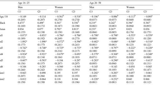
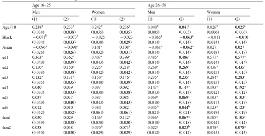
wages mean hourly occupation wage are similar to those specified for the current drug use probit, except that we exclude religious attendance and housing tenure Žrented . The results for unemployment and occupational attainment are sum-. marised in Tables 7 and 8, respectively. It is here that the different experiences of men. and women become particularly apparent.
The impact of socio-economic factors on unemployment and occupational attainment is more or less as expected. Not surprisingly, the educational variables are highly significant in both sets of estimates, particularly for the older cohorts. Looking at the impact of age, the results suggest that older respondents are less likely to be currently unemployed and tend to have a higher wage. In all cases, those of Black origin tend to have a higher probability of being currently unemployed, and Black men tend to have lower wages when compared to Whites. The results for Asians vary according to gender. Young Asian women and older Asian men tend to have a higher probability of unemployment when compared to whites, although the estimated coefficients for young Asian men and older Asian women are not significant. However, when we consider wages, these results are reversed, and it is young Asian women who tend to have higher wages than
Ž . Ž
Whites, whereas Asian men young or old tend to have lower wages the .
estimated coefficient for older women is not statistically significant . Residence in the inner city is positively associated with current unemployment, but for the older cohort, there is a statistically significant positive association with wages. We also observe that older individuals who report frequent alcohol consumption tend to
Ž
have higher wages this is consistent with the literature although we do not distinguish between frequent drinking and problem drinking, and nor do we allow
.
Focusing on the relationship between drug use and labour market outcomes, the lagged effects of past drug use vary between age, gender and the groups of drugs considered. Looking first at participation, we see that the past use of recreational
ˆ
Ž .
or soft drugs d31 tends not to be significantly associated with current unemploy-ment, except for young women where the association is positive, but of marginal
ˆ
Ž .
significance. However, past use of hard or dependency drugs d32 has a signifi-cant positive impact on the probability of current unemployment, except for older
Ž .
women and young men for model 1 , where the estimated coefficients are not significantly different from zero. Overall, there is strong evidence of long-term damage to employment prospects from the use of hard or dependency drugs. In addition to the lagged effects, Table 7 also shows significant correlations between
Ž .
current drug use and unemployment r
ˆ
d u , although it is difficult to unravel this association.When we consider the impact of drug use on occupational attainment for those in work, we find very little evidence of any relationship. Where there is some evidence, the results vary between genders. For example, whereas there is a
ˆ
Ž . negative relationship between the past use of soft or recreational drugs d41 and the wages of older men, we observe a positive relationship between these variables for older women. However, we find no significant association between past soft or recreational drug use and wages for the younger cohort, and no association
ˆ
Ž .
between past hard or dependency drug use d42 and wages for any group considered. The one exception is curious as we find a positive association between
Ž
the past use of hard drugs and the wages of young women although the estimated .
coefficient is small and of marginal significance . This result is in line with some
Ž .
of the literature e.g., Kaestner, 1994b , and is also supported by the correlation between current drug use and wages. In all cases, except for young women, the
Ž .
estimated correlation coefficient r
ˆ
d w is not significant, although it is positive for all but older men, and positive and statistically significant for young women.()
The probability of current unemployment: probit estimates
Age 16–25 Age 26–50
Men Women Men Women
Ž .1 Ž .2 Ž .1 Ž .2 Ž .1 Ž .2 Ž .1 Ž .2
b c a b b c
Ager10 y0.149 y0.114 y0.561 y0.518 y0.106 y0.086 y0.113 y0.095
Ž0.205. Ž0.207. Ž0.270. Ž0.274. Ž0.037. Ž0.037. Ž0.048. Ž0.048.
a a c b a a a a
Black 0.473 0.498 0.363 0.356 0.219 0.242 0.396 0.383
Ž0.169. Ž0.171. Ž0.187. Ž0.190. Ž0.082. Ž0.083. Ž0.094. Ž0.093.
a a a a
Asian 0.034 0.077 0.792 0.813 0.233 0.267 0.021 0.036
Ž0.135. Ž0.138. Ž0.158. Ž0.160. Ž0.084. Ž0.085. Ž0.176. Ž0.175.
a a a a a a a a
ed1 y0.873 y0.851 y0.786 y0.706 y0.798 y0.798 y0.553 y0.559
Ž0.189. Ž0.192. Ž0.269. Ž0.273. Ž0.080. Ž0.080. Ž0.121. Ž0.120.
a a b b a a a a
ed2 y1.092 y1.090 y0.572 y0.596 y0.682 y0.686 y0.508 y0.510
Ž0.177. Ž0.177. Ž0.241. Ž0.241. Ž0.081. Ž0.081. Ž0.123. Ž0.122.
a a a a a a a a
ed3 y0.742 y0.748 y0.725 y0.733 y0.789 y0.797 y0.222 y0.220
Ž0.154. Ž0.156. Ž0.216. Ž0.217. Ž0.100. Ž0.099. Ž0.119. Ž0.118.
a a a a a a a a
ed4 y0.924 y0.921 y0.679 y0.691 y0.379 y0.368 y0.265 y0.248
Ž0.132. Ž0.134. Ž0.184. Ž0.183. Ž0.071. Ž0.071. Ž0.088. Ž0.088.
a a a a a a
ed5 y0.607 y0.583 y0.184 y0.207 y0.283 y0.290 y0.416 y0.413
Ž0.156. Ž0.157. Ž0.207. Ž0.207. Ž0.095. Ž0.094. Ž0.132. Ž0.131.
ed6 y0.346 y0.283 y0.560 y0.565 y0.145 y0.143 y0.054 y0.045
Ž0.244. Ž0.242. Ž0.393. Ž0.391. Ž0.106. Ž0.105. Ž0.147. Ž0.147.
c c
fam1 y0.043 y0.098 0.195 0.197 y0.202 y0.203 y0.057 y0.061
Ž0.207. Ž0.206. Ž0.193. Ž0.193. Ž0.105. Ž0.105. Ž0.108. Ž0.108.
a a
fam2 y0.012 y0.064 0.118 0.104 y0.220 y0.232 0.043 0.066
()
fam4 0.299 0.325 0.367 0.339 y0.122 y0.119 y0.154 y0.134
Ž0.247. Ž0.248. Ž0.198. Ž0.194. Ž0.102. Ž0.102. Ž0.110. Ž0.110.
a a
fam5 0.527 0.444 0.037 0.010 y0.070 y0.059 0.025 0.025
Ž0.178. Ž0.178. Ž0.251. Ž0.252. Ž0.073. Ž0.073. Ž0.111. Ž0.111.
b b a a a a
Married y0.238 y0.207 y0.353 y0.352 y0.697 y0.690 y0.665 y0.646
Ž0.150. Ž0.150. Ž0.167. Ž0.168. Ž0.078. Ž0.078. Ž0.093. Ž0.092.
a a b b a a a a
City 0.305 0.296 0.280 0.293 0.399 0.408 0.291 0.291
Ž0.096. Ž0.097. Ž0.117. Ž0.117. Ž0.053. Ž0.053. Ž0.071. Ž0.071.
c b
freqdrnk 0.104 0.069 y0.222 y0.272 y0.115 y0.125 y0.019 y0.031
Ž0.118. Ž0.119. Ž0.175. Ž0.177. Ž0.059. Ž0.058. Ž0.083. Ž0.081.
a a a a a a
Year 1996 y0.093 y0.103 y0.441 y0.438 y0.150 y0.151 y0.291 y0.278
Ž0.109. Ž0.110. Ž0.126. Ž0.125. Ž0.058. Ž0.058. Ž0.071. Ž0.071.
Lagged drug effects
c c
ˆ
d31 0.116 0.178 0.317 0.327 y0.039 0.010 y0.002 0.119
Ž0.131. Ž0.152. Ž0.165. Ž0.181. Ž0.067. Ž0.073. Ž0.096. Ž0.094.
a b a a a
ˆ
d32 0.307 0.450 0.697 0.476 0.392 0.342 0.167 0.078
Ž0.212. Ž0.120. Ž0.322. Ž0.181. Ž0.124. Ž0.076. Ž0.216. Ž0.152.
Constant y0.083 y0.221 0.429 0.335 0.069 y0.048 y0.579 y0.685
Ž0.431. Ž0.441. Ž0.536. Ž0.544. Ž0.173. Ž0.173. Ž0.215. Ž0.217.
a c c a a c b
rˆd u 0.167 0.115 0.145 0.119 0.237 0.200 0.121 0.157
Ž0.058. Ž0.064. Ž0.081. Ž0.091. Ž0.039. Ž0.043. Ž0.069. Ž0.067.
N 1259 1259 1255 1255 6037 6037 5357 5357
()
Determinants of occupational attainment: regression estimates
Age 16–25 Age 26–50
Men Women Men Women
Ž .1 Ž .2 Ž .1 Ž .2 Ž .1 Ž .2 Ž .1 Ž .2
a a a a a a a a
Ager10 0.238 0.233 0.242 0.236 0.040 0.041 0.026 0.025
Ž0.038. Ž0.038. Ž0.035. Ž0.035. Ž0.005. Ž0.005. Ž0.006. Ž0.006.
b b a a
Black y0.071 y0.073 y0.025 y0.023 y0.065 y0.063 y0.011 y0.010
Ž0.034. Ž0.033. Ž0.030. Ž0.029. Ž0.014. Ž0.014. Ž0.014. Ž0.014.
a a a a a a
Asian y0.096 y0.098 0.101 0.108 y0.061 y0.062 0.027 0.027
Ž0.026. Ž0.026. Ž0.032. Ž0.031. Ž0.014. Ž0.014. Ž0.018. Ž0.017.
a a a a a a a a
ed1 0.363 0.362 0.407 0.399 0.485 0.486 0.577 0.577
Ž0.040. Ž0.039. Ž0.043. Ž0.042. Ž0.014. Ž0.014. Ž0.014. Ž0.014.
a a a a a a a a
ed2 0.150 0.150 0.225 0.218 0.269 0.269 0.436 0.435
Ž0.038. Ž0.038. Ž0.042. Ž0.042. Ž0.014. Ž0.014. Ž0.015. Ž0.015.
a a a a a a a a
ed3 0.132 0.131 0.150 0.146 0.235 0.235 0.284 0.283
Ž0.035. Ž0.035. Ž0.040. Ž0.039. Ž0.014. Ž0.014. Ž0.015. Ž0.015.
a a a a
ed4 0.040 0.039 0.097 0.092 0.147 0.147 0.193 0.192
Ž0.033. Ž0.033. Ž0.038. Ž0.038. Ž0.013. Ž0.013. Ž0.012. Ž0.012.
a a a a
ed5 0.037 0.037 0.087 0.085 0.069 0.069 0.103 0.103
Ž0.040. Ž0.040. Ž0.043. Ž0.043. Ž0.018. Ž0.018. Ž0.017. Ž0.017.
b b a a
ed6 0.012 0.010 0.084 0.082 0.045 0.044 0.123 0.123
Ž0.052. Ž0.052. Ž0.061. Ž0.061. Ž0.021. Ž0.021. Ž0.019. Ž0.019.
a a a a a a
fam1 0.030 0.029 0.146 0.142 0.066 0.067 0.105 0.105
Ž0.039. Ž0.038. Ž0.030. Ž0.030. Ž0.018. Ž0.018. Ž0.014. Ž0.014.
b b c b a a
fam2 0.038 0.038 0.070 0.073 0.022 0.023 0.078 0.078
()
fam4 0.044 0.049 y0.014 y0.008 y0.004 y0.004 y0.002 y0.002
Ž0.048. Ž0.048. Ž0.033. Ž0.033. Ž0.017. Ž0.017. Ž0.015. Ž0.015.
b b b b
fam5 0.003 0.002 y0.045 y0.046 0.027 0.028 0.032 0.031
Ž0.040. Ž0.040. Ž0.035. Ž0.035. Ž0.011. Ž0.011. Ž0.012. Ž0.012.
a a
Married 0.010 0.013 y0.008 y0.007 0.052 0.053 y0.001 y0.001
Ž0.028. Ž0.028. Ž0.024. Ž0.024. Ž0.014. Ž0.014. Ž0.012. Ž0.012.
a a b b
City y0.017 y0.019 y0.011 y0.013 y0.055 y0.055 y0.020 y0.021
Ž0.020. Ž0.021. Ž0.018. Ž0.018. Ž0.009. Ž0.009. Ž0.009. Ž0.009.
a a a a
freqdrnk 0.034 0.034 y0.011 y0.015 0.024 0.024 0.040 0.040
Ž0.021. Ž0.021. Ž0.020. Ž0.020. Ž0.008. Ž0.008. Ž0.009. Ž0.009.
c b
Year 1996 y0.001 0.001 y0.033 y0.035 y0.012 y0.011 y0.011 y0.011
Ž0.019. Ž0.019. Ž0.017. Ž0.017. Ž0.008. Ž0.008. Ž0.008. Ž0.008.
Lagged drug effects
b c a a
ˆ
d41 y0.006 y0.002 0.008 0.019 y0.020 y0.018 0.032 0.036
Ž0.024. Ž0.027. Ž0.021. Ž0.024. Ž0.009. Ž0.010. Ž0.011. Ž0.011.
c ˆ
d42 y0.068 y0.013 y0.017 0.051 y0.011 y0.019 0.026 0.022
Ž0.051. Ž0.025. Ž0.060. Ž0.026. Ž0.020. Ž0.013. Ž0.022. Ž0.015.
Constant 1.136 1.144 0.981 0.993 1.536 1.532 1.401 1.406
Ž0.081. Ž0.081. Ž0.078. Ž0.078. Ž0.028. Ž0.028. Ž0.029. Ž0.029.
c
rˆd w 0.015 0.000 0.095 0.076 y0.005 y0.019 0.042 0.032
Ž0.048. Ž0.055. Ž0.049. Ž0.055. Ž0.026. Ž0.030. Ž0.033. Ž0.033.
Mean LL y1.6179 y1.8131 y1.2125 y1.3608 y1.2577 y1.3486 y0.9102 y1.0057
N 1259 1259 1255 1255 6037 6037 5357 5357
estimated impact of lagged drug use. The bias will only be serious if drug use has its main effects on wages within occupations rather than on transitions between occupations. We find this unlikely for two reasons. Firstly, our occupational classification is very fine, so most individual careers will normally involve several
Ž .
changes of occupation. Secondly, the relatively small and mainly positive
Ž .
impacts estimated from US actual wage data see Kaestner, 1994b are broadly in line with our findings.
6. Concluding remarks
In this paper, we have used data from the BCS to explore the relationship between illicit drug use and two labour market outcomes: unemployment and occupational attainment.
One of our objectives was to explore a previously hypothesised lifespan perspective to the relationship between drug use and labour market outcomes ŽKandel et al., 1995 . This suggests that the positive returns to drug use found in. previous studies will only be apparent for individuals in the early stages of their career. We find little evidence to support this hypothesis, indeed, like Burgess and
Ž .
Propper 1998 , if anything our results contradict it. We find that this result is also gender-specific, and only relevant to the past use of recreational or soft drugs. In particular, we only find a positive association between past soft drug use and the wages of older women. There is practically no evidence to suggest any positive
Ž
returns to drug use for the younger cohort, particularly for men in all cases, the .
estimated coefficients are negative for men .
What we do find is a highly significant relationship between hard drug use and unemployment, where it represents long-term harm to employment prospects. We suggest that taking the relationship between drug use and unemployment into account may help explain why recent work has failed to find any significant
Ž .
negative relationship between drug use particularly hard drugs and earnings. We
Ž .
have shown that drug use particularly hard or dependency drugs greatly increases the risk of unemployment, and any association with earnings for those in work therefore misses much of the impact. The strong evidence of the adverse affects of drug use on employment prospects overwhelms the mild estimated positive association between past soft drug use and occupational attainment for women.
even if it is from the point of view of the individual employer. There are other Ž
aspects of drug use in the workplace as, e.g., in the work of Kaestner and .
Grossman, 1998 on workplace accidents , which we have not been able to consider but may further support the need for workplace drug testing. This would, of course, be highly specific to the nature of the job concerned. However, given our results, we believe that policy conclusions should be mainly concerned with the implications of drug use for unemployment rather than the impact on produc-tivity for those who are in work. Regardless of the direction of causation between drug use and unemployment, it is most likely that those drug users who are
Ž unemployed and need to maintain a habit generate considerable social costs e.g.,
.
through acquisitive crime or prostitution . Governments have recognised the Ž benefits of targeting employment policies to help people get back into work e.g.,
.
Welfare to Work , and considerable public expenditure is committed to drug rehabilitation schemes. Perhaps, one conclusion that can be drawn is that there would be considerable benefits to be reaped if these two policies were better coordinated.
Acknowledgements
Material from Crown copyright records made available through the Home Office and the ESRC Data Archive has been used by permission of the Controller of Her Majesty’s Stationery Office. The authors are grateful to Mike Shields, and to two anonymous referees for helpful comments and suggestions. Any remaining errors and omissions are the sole responsibility of the authors.
References
Becker, G., Murphy, K., 1988. A theory of rational addiction. Journal of Political Economy 96, 675–700.
Berger, M., Leigh, J., 1988. The effect of alcohol use on wages. Applied Economics 20, 1343–1351. Burgess, S.M., Propper, C., 1998. Early health-related behaviours and their impact on later life
chances: evidence from the US. Health Economics 7, 381–399.
Culyer, A., 1973. Should social policy concern itself with drug abuse? Public Finance Quarterly 1, 449–456.
Fendrich, M., Vaughn, C.M., 1994. Diminished lifetime substance abuse over time: an inquiry into differential underreporting. Public Opinion Quarterly 58, 96–123.
French, M., Zarkin, G., 1995. Is moderate alcohol use related to wages? Evidence from four worksites. Journal of Health Economics 14, 319–344.
Gill, A., Michaels, R., 1991. The determinants of illegal drug use. Contemporary Policy Issues 9, 93–105.
Ž .
Hales, J., Stratford, N., 1997. 1996 British Crime Survey England and Wales : Technical Report. SCPR, London.
Hamilton, V., Hamilton, B., 1997. Alcohol and earnings: does drinking yield a wage premium? Canadian Journal of Economics 30, 135–151.
Harper, B., Haq, M., 1997. Occupational attainment of men in Britain. Oxford Economic Papers 49, 638–650.
Heien, D., 1996. Do drinkers earn less? Southern Economic Journal 63, 60–68.
Hoyt, G.M., Chaloupka, F.J., 1994. Effect of survey conditions on self-reported substance use. Contemporary Economics Policy 12, 109–121.
Kaestner, R., 1991. The effects of illicit drug use on the wages of young adults. Journal of Labor Economics 9, 381–412.
Kaestner, R., 1994a. The effect of illicit drug use on the labour supply of young adults. Journal of Human Resources 29, 126–155.
Kaestner, R., 1994b. New estimates of the effects of marijuana and cocaine use on wages. Industrial and Labor Relations Review 47, 454–470.
Kaestner, R., Grossman, M., 1998. The effect of drug use on workplace accidents. Labour Economics 5, 267–294.
Kandel, D., Chen, K., Gill, A., 1995. The impact of drug use on earnings: a lifespan perspective. Social Forces 74, 243–270.
Kenkel, D.S., Ribar, D.C., 1994. Alcohol consumption and young adults’ socioeconomic status. Brookings Papers on Economics Activity: Microeconomics, 119–175.
Labouvie, E., 1996. Maturing out of substance abuse: selection and self-correction. Journal of Drug Issues 6, 457–476.
MacDonald, Z., 1999. Illicit drug use in the UK: evidence from the British Crime Survey. British Journal of Criminology 39, 585–608.
MacDonald, Z., Pudney, S., 2000. Analysing drug abuse with British Crime Survey data: modelling
Ž .
and questionnaire design issues. Journal of Royal Statistical Society, Series C Applied Statistics 49, 95–117.
MacDonald, Z., Shields, M., 2000. The impact of alcohol use on occupational attainment in England. Economica, forthcoming.
McAllister, I., Makkai, T., 1991. Correcting for the underreporting of drug use in opinion surveys. International Journal of the Addictions 26, 945–961.
Mensch, B.S., Kandel, D.B., 1988. Underreporting of substance abuse in a national longitudinal youth cohort. Public Opinion Quarterly 52, 100–124.
Mullahy, J., Sindelar, J.L., 1991. Gender differences in labor market effects of alcoholism. American Economic Review 81, 161–165.
Mullahy, J., Sindelar, J.L., 1996. Employment, unemployment and problem drinking. Journal of Health Economics 15, 409–434.
Nickell, S., 1982. The determinants of occupational attainment in Britain. Review of Economic Studies 49, 43–53.
O’Muircheartaigh, C., Campanelli, P., 1998. The relative impact of interviewer effects and the sample
Ž
design effects on survey precision. Journal of the Royal Statistical Society, Series A Statistics in
.
Society 161, 63–77.
Parker, H., Measham, F., 1994. Pick ‘n’ mix: changing patterns of illicit drug use amongst 1990s adolescents. Drugs: Education, Prevention and Policy 1, 5–13.
Peck, D.F., Plant, M.A., 1987. Unemployment and illegal drug use. In: Heller, T., Gott, M., Jeffery, C.
ŽEds. , Drug Use and Misuse: A Reader. Wiley, Chichester, pp. 63–68..
Ramsay, M., Percy, A., 1996. Drug misuse declared: results from the 1994 British Crime Survey. Home Office Research Study 151 Home Office Research and Statistic Department, London. Ramsay, M., Percy, A., 1997. A national household survey of drug misuse in Britain: a decade of
Ramsay, M., Spiller, J., 1997. Drug misuse declared in 1996: key results from the British Crime Survey. Home Office Research Study 172 Home Office Research and Statistic Department, London.
Register, C., Williams, D., 1992. Labor market effects of marijuana and cocaine use among young men. Industrial and Labor Relations Review 45, 435–448.
Sickles, R., Taubman, P., 1991. Who uses illegal drugs? American Economic Review 81, 248–251. White, A., Malbon, G., 1995. 1994 British Crime Survey: Technical Report. OPCS Social Survey
Division, London.
Zarkin, G., Mroz, T., Bray, J., French, M., 1998a. The relationship between drug use and labor supply for young men. Labour Economics 5, 385–409.