Economies of scale and scope in higher education: a case of
comprehensive universities
Rajindar K. Koshal
a,*, Manjulika Koshal
baDepartment of Economics, Ohio University, Athens, OH 45701-2979, USA bManagement Sciences, Ohio University, Athens, OH 45701-2979, USA
Received 1 February 1998; accepted 1 July 1998
Abstract
This study empirically estimates a multiple-product fixed total cost function and output relationship for comprehensive universities in the United States. Statistical results based on data for 158 private and 171 public comprehensive
univer-sities suggest that there are both economies of scale and economies of scope in higher education. However,
product-specific economies of scope do not exist for all output levels and activities [JEL I22]. 1999 Elsevier Science Ltd. All rights reserved.
Keywords: Scale; Scope economies; Education cost
1. Introduction
Cost functions provide important information for pro-ducers to achieve efficiency in production. In the case of higher education, the question of economies of scale has been debated for over half of a century. Studies by Hashimoto and Cohn (1997), Koshal and Koshal (1995), Nelson and Heverth (1992), de Groot et al. (1991), Clot-felter et al. (1991), Getz et al. (1991), Hoenack (1990), Cohn et al. (1989), Brinkman (1990), Brinkman and Les-lie (1986) and Friedman (1955) have conflicting con-clusions regarding economies of scale. Our study explores different dimensions of economies of scale by estimating a multiple-product fixed total cost function. In the 1970s, two studies (Verry & Layard, 1975; Verry & Davies, 1976) also suggested the use of multiple-output total cost functions. However, recent studies also suggest that institutions of higher education produce multiple products (Jimenez, 1986; Cohn et al., 1989; Cohn, & Geske, 1990; Lloyd et al., 1993; Hashimoto & Cohn, 1997; Johnes, 1997). In addition, the quality of
edu-* Corresponding author. Tel.:11-740-593-2038; Fax:1 1-740-593-0181; E-mail: [email protected]
0272-7757/99/$ - see front matter1999 Elsevier Science Ltd. All rights reserved. PII: S 0 2 7 2 - 7 7 5 7 ( 9 8 ) 0 0 0 3 5 - 1
cation, whether perceived or real, is different at different institutions (Koshal & Koshal, 1995). For example, one year of education at Amherst College is not the same as one year of education at Huntington College. Therefore, the cost and output relationship must make adjustments for various outputs and for quality variations among institutions. In addition to the single-output method, these studies had other drawbacks. First, some used the assumption that all the institutions in a cross-section analysis have the same objectives. It would be unreason-able to assume that the goal for all universities is to pro-vide the same educational experience. One needs to account for such differences in relating cost to outputs. Second, most of the studies did not test their results for the presence of heteroscedasticity.
2. Model
In this study, we model our multiple-product cost function following the work of Baumol et al. (1982), Mayo (1984), Cohn et al. (1989), de Groot et al. (1991), Nelson and Heverth (1992), Dundar and Lewis (1995) and Hashimoto and Cohn (1997). Instead of a translog function, we assume that total cost (TC) of education output at an institution is represented by a flexible “fixed” cost quadratic function (FFCQ) of the follow-ing form:
where TC is the total cost of producing k products, a0is
a constant, and aiand bij are the coefficients associated
with various output variables. Qiis the output of the ith
product. c1 and c2 are the coefficients of two dummy
variables, DGand DR. DGhas a value of one if graduate
output is non-zero, otherwise it takes a value of zero. Similarly, DRis defined for the level of research activity.
The terms d1, d2and d3are the coefficients of the control
program classification dummies C1, C2and C3. The
Car-negie Commission has divided comprehensive univer-sities into four classifications (Carnegie Foundation for the Advancement of Teaching, 1987). C1is a dummy if
a university is public and over half of their baccalaureate degrees are awarded in two or more occupational or pro-fessional disciplines. C3is similarly defined for private
universities. C2and C4are dummy variables for public
and private institutions. In our study, C4represents the
reference group. These institutions award more than half of their baccalaureate degrees in occupational or pro-fessional disciplines. In addition, they may also offer graduate education through the masters degree. C1, C2
and C3take values of one or zero according to an
obser-vation belonging to the particular classification. The coefficient f of the dummy PHD is for institutions that offer Ph.D. degrees. The PHD variable takes a value of one for institutions that offer Ph.D.; otherwise, it takes a value of zero. V is a random error term. The cost func-tion of Eq. (1) permits us to estimate both economies of scale and economies of scope.
Generally, in the United States for higher education, there are three products: QU, undergraduate students; QG,
graduate students; and QR, research activities. Following
Baumol et al. (1982), Cohn and Geske (1990) and Hashi-moto and Cohn (1997), we first define the average incremented cost (AIC) for undergraduate output as
AICU5
TC{QU,QG,QR}2TC{0,QG,QR} QU
(2)
where TC{QU, QG, QR} is the total costs of producing
QUunits of undergraduate students, QGunits of graduate
students and QRunits of research. TC{0, QG, QR} is the
total cost when output for product U is zero. Similarly, average incremental costs (AICGand AICR) for products
G and R are defined. As in the case of a single product, the economies of scale are measured by the ratio of aver-age to marginal costs. Economies of scale are said to exist if this ratio is greater than one. The product-specific economies of scale for product U is defined as
EU5
AICU
MCU
(3)
where MCU5∂TC/∂QUis the marginal cost of
produc-ing product U. If EUis greater (smaller) than one,
econ-omies (diseconecon-omies) of scale are said to exist for the product U. Ray (overall) economies of scale (RE) may exist when the quantities of the product are increased proportionally. Ray economies of scale are defined as follows:
RE5Q TC{QU,QG,QR} UMCU1QGMCG1QRMCR
(4)
Ray economies (diseconomies) of scale are said to exist when RE is greater (less) than one.
In any production process, economies of scope are present when there are cost efficiencies to be gained by joint production of multiple products, rather than by being produced separately. Following Dundar and Lewis (1995) and Hashimoto and Cohn (1997), economies of scope are divided into global and product-specific econ-omies of scope. The degree of global econecon-omies (GE) of scope in the production of all products is defined as
GE5 (5)
TC{QU,0,0}1TC{0,QG,0}1TC{0,0,QR}2TC{QU,QG,QR}
TC{QU,QG,QR}
Global economies (diseconomies) of scope are said to exist if GE is greater (less) than zero. Cost advantages due to production of each product jointly with the other outputs are called product-specific economies of scope (PSE). For example, for product U, this is given by
PSEU5 (6)
TC{QU,0,0}1TC{0,QG,QR}2TC{QU,QG,QR}
TC{QU,QG,QR}
Product-specific economies (diseconomies) of scope associated with product U are said to exist if PSEU is
greater (less) than zero.
3. Data
collected from Management Ratios No. 7 for Colleges and Universities (1993)1and Barron’s Profiles of
Amer-ican Colleges (1991). There are 635 comprehensive uni-versities in the United States. However, a complete set of data for this analysis is available only for 329 of these institutions. In higher education, as pointed out by Cohn et al. (1989), there is no consensus on the appropriate measures of output. For the purpose of our analysis, we assume three outputs in higher education: (1) the number of full-time equivalent undergraduate students (QU), (2)
the number of full-time equivalent graduate students (QG) and (3) the level of research activities measured
in dollars (QR). QU includes all undergraduate students
enrolled as freshmen, sophomores, juniors and seniors.
QGincludes students enrolled in masters-level and
doc-torate-level classes. We recognize that full-time equival-ent enrollmequival-ent (FTE) may not be the ideal measure of output, but it is an important improvement over just the absolute number of students used by some of the pre-vious studies. Thus, in the absence of any better data, we have selected QU and QG in FTE units as our best
measurements of the two teaching outputs.
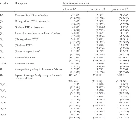
In regards to the research output, the measurement of which is equally (or perhaps even more) controversial, the best measure available for this study is the amount of research funds that the faculties expend. The total cost variable used here (TC) is measured by a university’s current expenditure. Definitions of variables used in this study, along with some basic descriptive statistics, are presented in Table 1.
For a measure of quality (Q), we use the average total scores on the Scholastic Aptitude Test (SAT) of entering freshmen2. The average SAT score signals the quality
of an institution to prospective students and their future employers (Koshal et al., 1994; Koshal, & Koshal, 1995). To purchase a higher-quality educational experi-ence, students/parents are willing to pay more at insti-tutions with higher average SAT scores. In a study, Koshal and Koshal (1995) have shown that SAT and the quality index for colleges by US News and World
Reports generate quite similar results in regression
analysis.
1The Management Ratios data are from the US Department of Education, National Center for Education Statistics (1993). 2SAT scores are not available for a few institutions. By using the data of Langston and Watkins (1980) for SAT equivalencies of ACT scores, Harford and Marcus (1986) suggest the follow-ing regression equation for convertfollow-ing ACT scores to SAT scores:
SAT5309.91114.89ACT10.226(ACT)2
10.0086(ACT)3 Using this equation, we estimate SAT scores for the institutions for which the only ACT scores are reported.
4. Statistical results
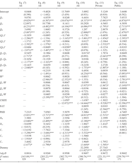
Using the above data and applying the multiple regression technique, we first estimate the above quad-ratic multi-product total cost function. The results of this analysis are summarized in Table 2 as Eq. (7). The values in parentheses below the coefficients in Table 2 are t-values, Adj-R2 is the coefficient of determination
adjusted for the degrees of freedom. The F-ratio tests the overall fit of the equation. In Table 2, *** denotes a 1% level of significance, ** denotes a 5% level of signifi-cance, * denotes a 10% level of signifisignifi-cance, and @ rep-resents a 15% level of significance.
Statistically, the results of Eq. (7) in Table 2 are sig-nificant and the coefficients have the expected sign. These results suggest that the economies of scale exist in producing undergraduate, graduate student output and research activities. Yet, as explained below, this equation does not tell the entire story about the relationship between cost and output.
Jimenez (1986) and Hashimoto and Cohn (1997) sug-gest that including an index of input prices in the total cost function is important since, in a cross-section data set, the institutions are located all over the country. Each university may face different factor costs that would then influence total cost. Because faculty salaries, including instructional material, constitute a high proportion of the total cost of education, they are the most predominant factor cost. We re-estimate our cost function including average faculty salary plus instructional material per fac-ulty member (FS). The results are summarized in Eq. (8) in Table 2. Since institutions can control total cost by varying the number of students per faculty member, we estimate Eq. (9) by adding class size (CSIZE). In Eq. (10) we add the SAT variable to test whether the quality of entering students has any effect upon total cost. Also included in Eq. (10) is a dummy for institutions that are primarily oriented toward engineering and medical edu-cation. To test for the presence of heteroscedacity, we apply the RESET test (Ramsey, 1969) to the residuals of Eqs (7) to (10). The test statistics indicate the presence of heteroscedacity. Therefore, the coefficients of these Eqs (7)–(10) are unbiased but inefficient, thus invalidat-ing the test of significance.
Since public and private institutions have different objectives, we suggest estimating the cost function separ-ately for private and public institutions. Following this approach, Eq. (11) summarizes the results only for priv-ate institutions while Eq. (12) gives results for public institutions. The RESET test suggests that the residuals of Eq. (11) as well as those of Eq. (12) are homoscedas-tic. Therefore, the coefficients of these equations are unbiased and efficient. The discussion that follows uses the results of Eqs (11) and (12).
Table 1
Definition of variable and summary statistics
Variable Description Mean/standard deviation
all: n5329 private: n5158 public: n5171
TC Total cost in millions of dollars 42.1617 32.1411 51.4205
(32.0721) (26.1320) (34.2698)
QU Undergraduate FTE in thousands 3.9487 2.2432 5.5253
(3.0417) (1.2773) (3.3374)
QG Graduate FTE in thousands 0.8692 0.59402 1.1235
(1.0789) (0.7693) (1.2506)
QR Research expenditure in millions of dollars 0.9891 0.4843 1.4556
(3.2618) (2.8256) (3.5634)
Q2
U (Undergraduate FTE)2 24.8160 6.6491 41.6018
(43.1002) (9.1335) (54.0085)
Q2
G (Graduate FTE)2 1.9161 0.9409 2.8171
(5.2497) (2.6016) (6.7248)
Q2
R (Research expenditure)2 11.5851 8.1682 14.7422
(82.7928) (93.7948) (71.2729)
SAT Average SAT score 881.3071 925.8994 840.1050
(127.5664) (108.7191) (130.1000)
CSIZE Average class size 16.1641 15.0380 17.2047
(3.8505) (3.6256) (3.7682)
SF Average faculty salary in hundreds of dollars 55.7872 54.7603 56.7361
(15.5623) (16.1070) (15.0263)
SF2 Square of average faculty salary in hundreds 3353.67 3256.49 3443.45 of square dollars
(2114.63) (2131.48) (2101.20)
QU·QG 5.5142 1.8899 8.8629
(12.3984) (3.9933) (16.0740)
QU·QR 6.2291 2.3390 9.823
(24.3170) (16.7828) (29.2183)
QG·QR 1.9282 1.0294 2.7586
(9.2781) (8.4762) (9.9181)
QU·SF 237.7131 128.4762 338.6453
(242.7062) (106.3684) (286.1256)
QG·SF 52.8275 34.2992 69.9473
(77.8858) (47.8555) (94.7381)
QR·SF 59.3355 35.4181 81.4345
(206.6608) (208.4771) (203.0780)
(12). Thus, our discussion will mainly concentrate on comparing the private education costs with those of pub-lic education costs.
In Tables 3 and 4, we provide the marginal cost of each product for different levels of output along a pro-portional output ray. These marginal cost values are cal-culated at the mean values of the relevant variables. An examination of the estimates in Tables 3 and 4 for priv-ate institutions suggests that, for all levels of output, the marginal cost of graduate FTE is higher than that for undergraduate FTE. For public institutions, the marginal cost for graduate output is higher than the undergraduate marginal cost only at and beyond the mean value of out-put. This is consistent with the practice at many public higher educational institutions of offering most of the
master-level courses combined with undergraduate level, especially in the cases where graduate output is low. The marginal cost for undergraduate FTE declines as output level increases. On the other hand, the marginal cost of graduate FTE and research activity increases as output level increases. For example, in the case of private insti-tutions, the marginal cost for graduate FTE is US$12 537 at the 50% level of mean output and US$18 526 for a 300% level of mean output.
insti-Table 2
Summary of regression results
Eq. (7) Eq. (8) Eq. (9) Eq. (10) Eq. (11) Eq. (12)
All All All All Private Public
Intercept 0.8468 29.4028 13.7689 3.8892 5.1249 3.6680
(0.390) (21.682) (3.439) (0.931) (0.810) (0.582)
QU 9.0781 6.8539 8.8248 6.4416 7.7825 5.0533
(9.029)*** (6.507)*** (10.074)*** (8.337)*** (3.065)*** (4.874)***
QG 12.0971 10.7788 8.1411 10.2920 6.5403 6.3050
(6.231)*** (4.482)*** (4.104)*** (6.086)*** (1.795)* (2.713)***
QR 3.6981 1.0683 0.3726 1.207 2.8879 2.4871
(5.087)*** (1.245) (0.529) (2.000)** (1.076) (2.479)**
(QU)2 20.1839 20.0895 20.1740 20.1781 20.4858 20.1448
(22.286)** (21.336) (23.165)*** (23.801)*** (21.854)* (22.395)**
(QG)2 21.3712 20.7295 20.0804 0.0127 22.1964 0.1985
(22.392)** (21.579)@ (
20.211) (0.039) (22.532)** (0.534)
(QR)2 20.0484 20.0689 20.02807 0.0011 20.1234 20.0183
(22.071)** (23.487)*** (21.702)* (0.078) (21.325) (20.821)
QU·QG 0.5455 0.1904 0.0608 0.01747 1.7874 0.0689
(1.717)* (0.697) (0.271) (0.092) (2.643)*** (0.298)
QU·QR 20.1654 20.1320 20.0448 0.0106 20.5360 0.0698
(22.177)** (22.163)** (20.888) (0.245) (20.750) (1.256)
QG·QR 20.1415 0.0259 20.0885 20.2230 2.2720 20.1820
(22.040)** (0.143) (20.592) (21.753)** (1.807)* (21.188)
SF — 20.2319 0.1198 0.4936 0.0939 0.9580
(21.491)@ (0.931) (4.254)*** (0.564) (5.093)***
SF2 — 0.0042 0.0028 20.0015 0.0005 20.0051
(2.946)** (2.352)** (21.353) (0.334) (22.701)***
QU·SF — 0.0046 0.0047 0.0399 0.0612 0.0514
(0.334) (0.415) (3.937)*** (1.847)* (3.169)***
QG·SF — 0.0070 0.0064 20.0196 0.0664 20.0008
(0.180) (0.202) (20.725) (1.162) (20.021)
QR·SF — 0.0405 0.0290 0.0029 20.0277 20.0199
(3.199)*** (2.793)*** (0.312) (20.833) (21.304)
CSIZE — — 21.6507 21.6387 21.3022 22.0384
(212.872)*** (214.664)*** (29.520)*** (212.396)***
SAT — — — 0.0039 0.0103 20.0031
(1.245) (2.364)** (20.758)
PHD 7.2315 7.0583 5.5079 5.3084 2.1627 4.7485
(3.021)*** (3.717)*** (3.540)*** (4.013)*** (1.515)@ (2.060)**
DR 3.3001 3.2653 2.5294 1.9919 2.1999 20.0451
(2.040)** (2.489)** (2.348)** (2.180)** (2.115)** (20.029)
DG 20.0299 0.3432 21.3239 21.8027 21.4147 21.5402
(20.015) (0.219) (21.028) (21.648)@ (21.193) (20.887)
C1 213.6192 27.7822 27.3364 25.2131 2 0.0012
(25.298)*** (23.686)*** (24.313)*** (23.532)*** (0.001)
C2 25.9198 22.2531 22.3315 21.5060 2 —
(21.910)* (20.896) (21.153) (20.862)
C3 3.4682 2.9336 2.9578 1.9049 21.7952 —
(1.677)* (1.790)* (2.211)** (1.669)* (21.505)@
Dummy 2 2 2 32.2958 27.7343 —
(11.027)*** (9.392)***
Adj-R2 0.8816 0.9268 0.9508 0.9697 0.9672 0.9682
(F-ratio) {163.89}*** {203.22}*** {302.73}*** {390.76}*** {221.33}*** {259.79}***
n 329 329 329 329 158 171
Notes: Where applicable one tail test is applied.
Table 3
Marginal cost estimates for private institutions (MC in dollars)
% of output MC MCG/MCU
U MCG MCR
mean ratio
50 10 449 12 537 1.20 1.39
100 9761 14 510 1.49 1.40
150 9073 16 095 1.77 1.41
200 8385 17 293 2.06 1.43
250 7697 18 103 2.35 1.44
300 7009 18 526 2.64 1.46
Notes: MCU—marginal cost of undergraduate education; MCG—marginal cost of graduate education; MCR—marginal cost of research activities.
Table 4
Marginal cost estimates for public institutions (MC in dollars)
% of output MC MCG/MCU
U MCG MCR
mean ratio
50 7259 6541 0.90 1.42
100 6548 6821 1.04 1.49
150 5838 7102 1.22 1.55
200 5127 7383 1.44 1.61
250 4417 7664 1.74 1.68
300 3706 7945 2.14 1.74
Notes: MCU—marginal cost of undergraduate education; MCG—marginal cost of graduate education; MCR—marginal cost of research activities.
tutions is higher than at public educational institutions. However, it is interesting to observe that the marginal cost of graduate FTE at private educational institutions is more than double the marginal cost at public insti-tutions. The research marginal cost at both private and public institutions increases with the output level. The marginal cost of research at the public institutions is slightly higher compared with the marginal cost at priv-ate institutions.
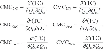
For the total cost function as formulated above, the estimated mean value of the outputs cross marginal cost (CMC) are defined as follows:
CMCUG5
ginal products, are given by the coefficients of the
corre-Table 5
Average costs for private institutions (AIC in dollars) % of output AIC AICG/AICU
U AICG AICR
mean ratio
50 10 993 7315 0.67 10.50
100 10 850 11 598 1.07 6.00
150 10 706 14 294 1.34 4.53
200 10 563 16 593 1.57 3.82
250 10 419 18 733 1.80 3.41
300 10 276 20 793 2.02 3.15
Notes: AICU—average integrated cost of undergraduate edu-cation; AICG—average integrated cost of graduate education; AICR—average integrated cost of research activities. Table 6
Average integrated cost for public institutions (AIC in dollars) % of output AIC AICG/AICU
U AICG AICR
mean ratio
50 7659 12 140 1.59 1.37
100 7348 9454 1.29 1.48
150 7038 8672 1.23 1.57
200 6727 8365 1.24 1.65
250 6417 8249 1.29 1.73
300 6106 8228 1.35 1.81
Notes: AICU—average integrated cost of undergraduate edu-cation; AICG—average integrated cost of graduate education; AICR—average integrated cost of research activities.
sponding interaction terms in Eqs (11) and (12), Table 2. A negative sign of the coefficients would imply that there is cost complementarity. A review of the results in Table 2 suggests that for private institutions, the coef-ficient of interaction terms for (QG·QR) and (QR·FS) only
have a negative sign. These terms are statistically insig-nificant. On the other hand, the coefficients of (QU·QR)
and (QG·QR) are positive and are significant at least at
the 5% level. This result implies substitutability between
QUand QRand also between QGand QR. For public
insti-tuitions, the negative sign is for the coefficient of interac-tion term (QU·QR), (QG·FS) and (QR·FS). The coefficients
of these terms are not statistically significant.
A major shortcoming with the multiple product case is that there is no direct analogy to the the “average cost” concept in the single output case (Cohn et al., 1989; Hashimoto & Cohn, 1997). However, as discussed earl-ier, the nearest analogy is provided by the average incremental cost (AIC). These values are listed in Tables 5 and 6. As is obvious from the marginal cost values for all output levels, the values of average incremental cost for graduate FTE is higher than the undergraduate FTE average incremental cost.
sug-Table 7
Ray economies of scale for private institutions % of output
ERAY EU EG ER
mean
50 0.65 1.05 0.58 7.58
100 1.22 1.11 0.80 4.29
150 1.81 1.18 0.89 3.21
200 2.43 1.26 0.96 2.67
250 3.11 1.35 1.03 2.36
300 3.87 1.47 1.12 2.16
Notes: ERAY—Ray economies of scale; EU—undergraduate edu-cation economies of scale; EG—graduate education economies of scale; ER—research activity economies of scale.
gests that, for private as well as public institutions, the AIC for undergraduate FTE declines as output level increases. For graduate FTE outcome is quite different. Graduate AIC at private institutions increases as output level increases, but at public institutions this declines with the increase of output level.
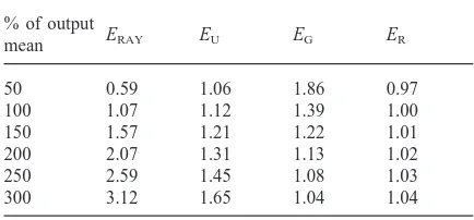
The estimates for the values of ray and product-spe-cific economies of scale are summarized in Tables 7 and 8. Ray economies and product-specific economies of scale occur when the scale coefficient is greater than one. The results indicate product-specific economies of scale for all products except graduate education at private institutions. Reviewing the values in Tables 7 and 8, one realizes that ray economies only apply when the output level is equal to or greater than the mean values of output for public and private institutions. Both undergraduate and graduate education at public institutions exhibit pro-duct-specific economies of scale. For private institutions, product-specific economies of scale are present for undergraduate education, but graduate education has dis-economies up to 200% of mean output level. It is inter-esting to note that research output exhibits economies of scale for private institutions and almost constant returns to scale for public institutions.
Table 8
Ray economies of scale for public institutions % of output
ERAY EU EG ER
mean
50 0.59 1.06 1.86 0.97
100 1.07 1.12 1.39 1.00
150 1.57 1.21 1.22 1.01
200 2.07 1.31 1.13 1.02
250 2.59 1.45 1.08 1.03
300 3.12 1.65 1.04 1.04
Notes: ERAY—Ray economies of scale; EU—undergraduate edu-cation economies of scale; EG—graduate education economies of scale; ER—research activity economies of scale.
Table 9
Economies of scope for private institutions % of output
ESG ESU ESG ESR
mean
50 1.13 20.03 0.07 1.17
100 0.57 20.06 20.03 0.64
150 0.33 20.08 20.10 0.44
200 0.19 20.12 20.16 0.34
250 0.08 20.15 20.22 0.28
300 20.01 20.18 20.28 0.23
Notes: ESG—global economies of scale; ESU—economies of scope for undergraduate education; ESG—economies of scope for graduate education; ESR—economies of scope for research activities.
Tables 9 and 10 list values of the coefficient of scope economies. As stated earlier, scope economies exist as long as the coefficient of economies of scope is positive. In Tables 9 and 10, for private as well as public insti-tutions, the coefficient of global economies of scope are positive except at 300% of the mean level of output for private institutions. Therefore, global economies of scope exist for the output range under consideration. The results for product-specific economies of scope are mixed. For research activity there are product-specific economies of scope at both private and public insti-tutions. These results imply product-specific diseconom-ies of scope for undergraduate and graduate education at private comprehensive universities. The results in Table 10 indicate product-specific diseconomies for undergrad-uate education only at an output level of 250% or higher of mean output. For illustration purposes, it is interesting to observe that for all outputs at 200% of their respective mean, the cost of production at comprehensive private universities that specialize in only one output is 19 times higher than it is for a university producing all three
out-Table 10
Economies of scope for public institutions % of output
ESG ESU ESG ESR
mean
50 0.38 0.11 0.12 0.26
100 0.21 0.05 0.07 0.15
150 0.14 0.02 0.05 0.10
200 0.10 0.00 0.03 0.08
250 0.07 20.02 0.03 0.06
300 0.05 20.04 0.02 0.05
puts. The corresponding figure for public institutions is 10.
5. Conclusions
Using data for 158 comprehensive private universities and 171 comprehensive public universities in the United States, this paper shows that it is possible to study econ-omies of scale, product-specific econecon-omies of scale, ray economies of scale and global economies of scope. The main findings of our study are as follows.
1. Holding all other things as being equal, the overall total cost is affected by class size. For example, on the average, if class size is increased by one student (FTE), ceteris peribus the overall total cost would decrease by US$1.30 million at public institutions and by US$2.04 million at private institutions.
2. Other things being equal, the quality of entering stu-dents as measured by SAT scores do affect total cost at private comprehensive universities.
3. Public institutions which offer a Ph.D. degree will, on average, have US$4.75 million in additional costs. However, at private institutions, the addition to total cost is US$2.16 million. This may be due to the fact that at private institutions, more of the costs related to doctorate programs are absorbed through research grants.
4. As observed by Nelson and Heverth (1992), Hashim-oto and Cohn (1997) and in our study also, the mar-ginal cost of graduate education is higher than that of undergraduate education teaching. However, our results for comprehensive universities implies that the ratio (MUG/MUU) is much smaller compared with
previous studies. In our study, this ratio varies between 1.20 and 2.64 for private institutions and between 0.90 and 2.14 for public institutions, com-pared with 3.0 to 5.3 in Nelson and Heverth’s study for the United States, and 50 in Hashimoto and Cohn’s study for Japanese private universities. 5. Our results indicate that ray economies of scale exist
for comprehensive universities. These results are quite similar to the findings by Cohn et al. (1989), Dundar and Lewis (1995) and Hashimoto and Cohn (1997). It may be noted that de Groot et al. (1991) found ray economies of scale for the large public research universities. Similarly Cohn et al. (1989) observed ray economies for the smaller universities. 6. As in the previous studies, our statistical estimates for
product-specific economies of scale for undergraduate and graduate education indicate mixed conclusions. Our results imply that there are product-specific econ-omies of scale for research at private institutions. For research at public institutions, after reviewing Table 8, one finds constant product-specific returns to scale.
In earlier studies, the results for undergraduate and graduate product-specific economies of scale have varied. For example, Cohn et al. (1989) reported pro-duct-specific economies of scale for graduate edu-cation and research in the public sector but no pro-duct-specific economies of scale for any of their output in the private sector. A study by Dundar and Lewis (1995) indicates the presence of product-spe-cific economies of scale for research but not for undergraduate and graduate education. They observed similar economies for all fields except for engineer-ing. A recent study of Japanese universities by Hashi-moto and Cohn (1997) concludes that there are pro-duct-specific economies of scale for undergraduate and graduate education for small universities and that product-specific economies of scale exist for research in large universities. According to our results, there are product-specific economies for undergraduate and graduate education at public universities for all levels of output. At private institutions, undergraduate edu-cation exhibits product-specific economies of scale at all levels. However, in the case of graduate education at private institutions, product-specific economies of scale are exhibited only at and beyond the 250% level of output.
7. Our results indicate that global economies of scope exist for the entire output range except at the 300% level output for private institutions. For research, pro-duct-specific economies of scope exist for all output levels at public and private institutions. The results for undergraduate and graduate education suggest both product-specific economies and diseconomies of scope depending on the output level as well as the type of institution. Overall, as regards to scope econ-omies, our results imply conclusions similar to those reached in earlier studies by Dundar and Lewis (1995), Cohn et al. (1989), Nelson and Heverth (1992) and Hashimoto and Cohn (1997).
Overall, our results suggest that comprehensive uni-versities in the United States can reap benefits from both scale and scope economies. Large comprehensive uni-versities appear to be more cost-efficient. Of course, beyond some level of output, inefficiencies may exist. But, based on the results in this study, we are not able to pinpoint any optimum level of output. In the future, with the availability of more refined data, many of the limitations of this study could be overcome and researchers might be able to estimate an optimum size for private and public comprehensive universities.
Acknowledgements
sugges-tions on an earlier draft of this paper. The authors also appreciate Dr Michael Williford’s help in supplying a part of the data set for this study. The authors are thank-ful to Robert D. Welch, PACE student, and Vipin Koshal for their help in the preparation of this paper. Any omis-sions are the responsibility of the authors.
References
Barron’s Profiles of American Colleges (1991). Barron’s Edu-cational Series, Inc. New York.
Baumol, W. J., Panzar, J. C., & Willig, R. D. (1982).
Contest-able markets and the theory of industry structure. New
York: Harcourt Brace Jovanovich.
Brinkman, P. T. (1990). Higher education cost functions. In S. A. Hoenack, & E. L. Collins (Eds.), The economies of
Amer-ican universities—management, operations, and fiscal environment (pp. 107–128). Albany, NY: State University
of New York Press.
Brinkman, P. T., & Leslie, L. L. (1986). Economies of scale in higher education: sixty years of research. Review of Higher
Education, 10, 1–28.
Carnegie Foundation for the Advancement of Teaching (1987).
A classification of institutions in higher education.
Prince-ton, NJ: Princeton University Press.
Clotfelter, C., Ehrenberg, R., Getz, M., & Siegfried, J. (1991).
Economic challenges in higher education. Chicago, IL:
Uni-versity of Chicago Press.
Cohn, E., & Geske, T. G. (1990). The economics of education (3rd ed.). Oxford: Pergamon Press.
Cohn, E., Rhine, S. L. W., & Santos, M. C. (1989). Institutions of higher education as multi-product firms: economies of scale and scope. Review of Economics and Statistics, 71, 284–290.
De Groot, H., McMahon, W. W., & Volkwein, J. F. (1991). The cost structure of American research universities. Review
of Economics and Statistics, 73, 424–431.
Dundar, H., & Lewis, D. R. (1995). Departmental productivity in American universities: economies of scale and scope.
Economics of Education Review, 14, 199–244.
Friedman, M. (1955). A survey of the empirical evidence of economies of scale. Comment in A Conference of the
Uni-versities National Bureau Committee for Economic Research, Business Concentration and Price Policy (pp.
230–238). Princeton, NJ: Princeton University Press. Getz, M., Siegfried, J. J., & Zhang, H. (1991). Estimating
econ-omies of scale in higher education. Economic Letters, 37, 203–208.
Harford, J. D., & Marcus, R. D. (1986). Tuition and U.S. private college characteristics: the hedonic approach. Economics of
Education, 5, 415–430.
Hashimoto, K., & Cohn, E. (1997). Economies of scale and scope in Japanese private universities. Education
Econom-ics, 5, 107–116.
Hoenack, S. A. (1990). An economist’s perspective on costs within higher education institutions. In S. A. Hoenack, & E. L. Collins (Eds.), The economics of American universities:
management, operations, and fiscal environment (pp. 129–
53). Albany, NY: State University of New York Press. Jimenez, E. (1986). The structure of educational costs:
multi-product cost functions for primary and secondary schools in Latin America. Economics of Education Review, 5, 25–39. Johnes, G. (1997). Costs and industrial structure in contempor-ary British higher education. Economic Journal, 107, 727–737.
Koshal, R. K., & Koshal, M. (1995). Quality and economies of scale in higher education. Applied Economics, 22, 3–8. Koshal, R. K., Koshal, M., Boyd, R., & Levine, J. (1994).
Tui-tion at Ph.D. granting instituTui-tions: a supply and demand model. Education Economics, 2, 29–44.
Langston, I. W., & Watkins, T. B. (1980). Sat–act equivalence.
Research memorandum 80-5. University Office of School
and College Relations, University of Illinois.
Lloyd, P. J., Morgan, M. H., & Williams, R. A. (1993). Amal-gamation of universities: are there economies of scale or scope? Applied Economics, 25, 1081–1092.
Management Ratios No. 7 for Colleges and Universities (1993). Boulder, CO: John Minter Associates.
Mayo, J. W. (1984). Multiproduct monopoly, regulation, and firm costs. Southern Economic Journal, 51, 208–218. Nelson, R., & Heverth, K. T. (1992). Effect of class size on
economies of scale and marginal costs in higher education.
Applied Economics, 24, 473–482.
Ramsey, J. B. (1969). Tests for specification errors in classical linear least squares regression analysis. Journal of the Royal
Statistical Society Series B, 31, 350–371.
US Department of Education, National Center for Education Statistics (NCES) (1993). Compact disk: Integrated Post-secondary Data System (IPEDS), Finance Survey, 1990–91; Final Release and Fall Enrollment Survey, 1990.
Verry, D., & Davies, B. (1976). University costs and outputs. Amsterdam: Elsevier Publishing.