Eliciting GPs’ preferences for pecuniary and
non-pecuniary job characteristics
Anthony Scott
∗Health Economics Research Unit, University of Aberdeen, Foresterhill, Aberdeen, AB25 2ZD, UK
Received 8 July 1999; received in revised form 31 July 2000; accepted 24 October 2000
Abstract
This study examines General Practitioners’ preferences for pecuniary and non-pecuniary job characteristics in the context of choosing a general practice in which to work. A discrete choice experiment is used to test hypotheses about the nature of the utility function. Marginal rates of substitution between income and non-pecuniary characteristics are calculated. The results suggest that policies aimed at influencing General Practitioners’ location choices should take account of both non-pecuniary and pecuniary factors, particularly out of hours work commitments. © 2001 Elsevier Science B.V. All rights reserved.
JEL classification:I110; C9; J2; J3
Keywords:Physician behaviour; Utility functions; Discrete choice models; Job characteristics
1. Introduction
The analysis of physician behaviour has focused on the role of financial incentives in influencing behaviour and on other factors influencing incomes, such as physician density. This approach is based on the neo-classical principal-agent model which assumes (amongst other things), that the contents of workers’ utility functions include leisure and the con-sumption of other goods and services, that income from work is important only in so far as it meets these objectives, and that workers experience disutility from work. This defines a central role for income and earnings-related incentives in influencing both the productivity of workers and their labour–leisure choices.
However, it has been recognised that this type of analysis may ignore non-pecuniary fac-tors that influence physician behaviour and labour supply. Economists in the classical tradi-tion argued that occupatradi-tional choice is determined by relative prices and the non-pecuniary
∗Tel.:+44-1224-681818/ext. 53866; fax:+44-1224-662994.
E-mail address:[email protected] (A. Scott).
attributes of work, where the equilibrium wage is the valuation of the non-pecuniary at-tributes (Ehrenberg and Smith, 1988; Rottenberg, 1971). For example,
“In the labour markets of Adam Smith. . . workers made occupational choice in terms
of comparative total net advantages, not in terms of comparative wages.” (Rottenberg, 1971)
Rottenberg argued that the ceteris paribusassumption in neo-classical models of
oc-cupational choice led to a heavy focus on pecuniary determinants of behaviour and that non-pecuniary factors were given less attention, not because they were less important than price, but because price fitted neatly into the more formal methods of quantitative analysis and calculus.
As well as theoretical arguments about the relevance of non-pecuniary characteristics, there is much empirical evidence from surveys in the non-economics literature about the various non-pecuniary characteristics that influence the job satisfaction and job choices of physicians (Scott, 1998). In the UK, the recent introduction of a salaried payment option for GPs and changes to the financing and organisation of out of hours care by GPs were designed to address low morale, stress and job dissatisfaction, and consequent problems of recruitment and retention. Such policies, however, do not fit easily with the traditional economic model of incentives based in principal-agent theory.
For these reasons, this paper takes a broader approach based on non-pecuniary job charac-teristics. In labour economics, a ‘job characteristics’ approach has been used in the context of testing the theory of compensating wage differentials (e.g. Sandy and Elliott, 1998). These studies have attempted to examine the role of pecuniary and non-pecuniary job char-acteristics, and have been most successful when attempting to value the risk of death or injury at work, to produce estimates of workers’ willingness to pay for risk reductions. (Gronberg and Reed, 1994; Herzog and Schlottmann, 1990; Kniesner and Leeth, 1991). However, few advances have been made when attempting to value other job characteristics (Cavalluzzo, 1991; Arai, 1994).
Although such an approach is not new in labour economics, it has yet to be incorporated into empirical work on physician behaviour. The basic income/leisure framework has been extended to include other arguments in the physician’s utility function. The most notable is the inclusion of various definitions of patients’ interests or ‘ethical’ concerns in the utility function (e.g. Evans, 1974; Feldstein, 1970; Zweifel, 1981; Dionne and Contandriopou-los, 1985). Others have suggested (though without explicit models), that factors such as autonomy, reputation and intellectual satisfaction may help to explain physician behaviour (Kristiansen, 1994). Other studies have included social norms and peer pressure as deter-minants of physician behaviour (Encinosa et al., 1997). However, these extensions have not been directly measured or tested in empirical work, which continues to be dominated by the role of financial incentives in influencing behaviour. Presumably, the reason for this is the difficulty in measuring these ‘psychological’ phenomena and the lack of secondary data sources that contain information about these variables. As a consequence, there is little evidence about what factors motivate GPs, and their implications for GPs’ decisions.
non-pecuniary arguments in the GPs’ utility function. The study is set in the context of GPs choosing a practice in which to work, and so the policy implications are concerned with the distribution of GPs and their location choices. A discrete choice experiment is used to test hypotheses about the contents of the utility function and to estimate GPs’ monetary valuations of non-pecuniary job characteristics.
2. A model of practice choice
The model concentrates on GPs’ choice of practice in which to work as a mechanism for revealing their preferences for pecuniary and non-pecuniary job characteristics. It is assumed that the utility function is defined over bundles of job characteristics (z) and leisure activities
(L), with each bundle of job characteristics representing a particular practice in which the
GP could potentially work.
GPs choose a practice at the beginning of their career as a GP or when they change jobs throughout their career. GPs can only choose one bundle of job characteristics given that they can only choose one practice at a time, and so the alternatives in the choice set
are mutually exclusive, withzexogenous at the time the choice is made.1 Hence, we are
concerned with an indirect utility function that indicates the maximised utility to be obtained
in a practice with characteristicsz(Peitz, 1995; Truong and Hensher, 1985).
Each practice in the choice set therefore comprises a bundle of job characteristics (z)
faced by thenth GP. With two practices (iandj),y∗
n is a latent variable representing the
difference in utility between the practices being compared. Since it is the choice that is
observed rather than the difference in utility,y∗
nis binary. Therefore,yn=1 ifyn∗>0 and
0 else, and
yn∗=(α+βzi+∂sn+εin)−(α+βzj+∂sn+εjn) (1)
whereα,βand∂are coefficients,sare socio-economic characteristics reflecting influences
on tastes andεis the random component of utility accounting for the analyst’s inability
to accurately observe individual’s behaviour (Manski, 1977; McFadden, 1974a,b). Further,
assume that there are taste variations, such that the marginal utility ofzdepends ons:
β =π+λsn (2)
This gives
yn∗=(α+π zi+λsnzi+∂sn+εin)−(α+π zj+λsnzj +∂sn+εjn) (3)
The discrete choice experiment used to estimate the model presents each GP with several pairs of scenarios. Multiple observations from each GP means that errors are not independent
and so an error termµncapturing random variation across GPs is included
y∗
n =(α+π zi+λsnzi+∂sn+εin+µn)
−(α+π zj+λsnzj +∂sn+εjn+µn) (4)
Taking differences for each pairwise choice (k), the equation to be estimated becomes
ykn∗ =π zk+λsnzk+εkn (5)
Terms common to both indirect utility functions drop out of the model (i.e.α,∂sn, andµn).
However, the inclusion of a constant term (α) and error term across respondents (µn)
can be used to test for mis-specification due to unobservable attributes and unobservable interaction terms between GPs’ socio-economic characteristics and attributes. The constant
term can be interpreted as the difference in the average utility of scenarioiandj, caused by
the use of a constant scenario, left/right bias or an omitted dummy variable that is a function of other included attributes (Scott, 2000). The model to be estimated then becomes
ykn∗ =α+π zk+λsnzk+εkn+µn (6)
This model was estimated using random effects probit regression. A full model was esti-mated including main effects and interaction terms for which hypotheses existed. This was then reduced to a more parsimonious model by excluding variables, one at a time, with
P-values greater than 0.10.
3. Methods
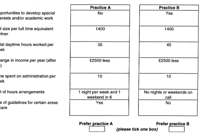
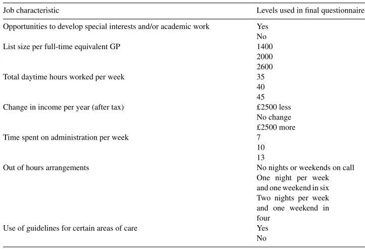
The stated preference technique of a discrete choice experiment was used to estimate the indirect utility function. The job characteristics and their definition were derived from existing economic models of GP behaviour and the non-economics literature, including surveys of factors influencing job satisfaction and job choice (Scott, 1997). Interviews with three full-time GP principals and from a random sample survey of 100 full-time GPs in England, conducted as part of pilot work to this study, further confirmed that the attributes we selected were relevant (see Fig. 1 and Table 1).
Seven attributes were included. The first was the net income offered by the practice. This was defined in terms of changes in income. If absolute income levels had been used, then results might have been sensitive to the GPs current level of income which varied across GPs. The levels were therefore defined as a reduction in income, no change in income, and as an increase in income. The interval between the levels is important to ensure some trading takes place. Too small an interval will mean that GPs do not consider the difference between levels to be important. Too large an interval may result in a dominant preference for income, where GPs are not prepared to trade income at all, and always choose the scenario with the highest level. In the first pilot questionnaire, GPs were asked when choosing a practice, how much income they would be prepared to forgo to work fewer hours per week, to have a lower list size, to spend fewer hours on administration, and to develop special interests. The mean amount of income GPs were willing to trade across these characteristics was £2668. The interval between income levels was therefore set at £2500.
Fig. 1. Example of a discrete choice.
1995). More patients on the list also generate more income under the current capitation system of GP payment in the UK. The interviews with GPs suggested it was interpreted as a measure of workload, rather than opportunities to increase patients’ utility or income. List size per GP was determined from the mean list size of full-time GPs in England (2051).
Table 1
Job characteristics and levels used in scenarios
Job characteristic Levels used in final questionnaire
Opportunities to develop special interests and/or academic work Yes No
List size per full-time equivalent GP 1400
2000 2600
Total daytime hours worked per week 35
40 45 Change in income per year (after tax) £2500 less
No change £2500 more
Time spent on administration per week 7
10 13
Out of hours arrangements No nights or weekends on call
One night per week and one weekend in six Two nights per week and one weekend in four
Use of guidelines for certain areas of care Yes No
Department of Health (Department of Health, 1994). Out of hours work was defined along two dimensions as the number of nights on call per week and the number of weekends on call, hence dummy variables were created to reflect the categorical but ordered nature of this variable (see Table 1). From the interviews and from previous surveys, this is the way most GPs would define the amount of work they do out of hours (Electoral Ballot Reform Services, 1992).
The sixth attribute was opportunities within the practice for the GP to invest in human capital, i.e. to undertake further postgraduate education, academic work or to have a special interest (Beardow et al., 1993; Roswell et al., 1995). This was interpreted as a proxy for intellectual satisfaction (Kristiansen, 1994). The final attribute was the extent to which clinical guidelines and peer review (e.g. through audit) are operational in the practice. This was included to reflect a concern for clinical autonomy. Whether the practice used guidelines or provided opportunities for the development of special interests were coded as binary variables.
The regression coefficients can be interpreted as scale transformations of the marginal utility of each attribute (Fowkes and Wardman, 1988). Of specific interest is the marginal utility of income and the marginal utility of time at work. The list size per GP and the existence of guidelines are both expected to have a negative effect on utility. The exis-tence of opportunities to invest in human capital is expected to have a positive effect on utility.
The extent to which GPs trade-off income for the other job characteristics gives an estimate of the monetary valuation of those characteristics. This is given by the marginal rate of substitution (MRS) between income and each of the other attributes (Small and Rosen, 1981; Propper, 1995). Trade-offs amongst other characteristics can also be estimated. This can be used in the reduced regression model to estimate the monetary valuation for specific sub-groups of GPs defined through the interaction terms. The MRS have important policy implications as, combined with the cost of altering each attribute, they can be used to find the most cost-effective policy to change GP utility and hence practice choices. The model can also be used to predict which set of job characteristics generates the highest utility, and used to predict the effect of changes in characteristics on utility.
The levels for each attribute were organised into scenarios using a factorial experimental
design. A full factorial design produced 35×22=243×4=972 scenarios. A fractional
factorial design produced 18 scenarios. This ensures an orthogonal design, i.e. that levels are varied independently thus minimising multicollinearity. One scenario was chosen to be constant (see ‘Practice A’ in Fig. 1), and the other 17 compared with it. Seventeen scenarios were too many for an individual to complete, and given the expected low response rate from GPs, the 17 scenarios were split randomly across four questionnaires, with three questionnaires with four choices and one with five. The four versions of the questionnaire were randomly allocated to each GP.
The questionnaire was piloted a second time on a random sample of 100 English GPs with a 30% response rate. As a result, a different comparator scenario was chosen since 90% of respondents were choosing scenario B, and the definition of the out of hours attribute was altered on the basis of more accurate information on the amount of out of hours care of GPs from the questionnaire.
Sample size was determined on the basis of the analysis of sub-groups, with a minimum
figure of between 30 and 100 individuals foreachsub-group of interest (Permain et al.,
1991). Previous conjoint analysis studies that have examined the effect of socio-demographic characteristics on preferences have sampled between 100 and 150 individuals and found that the numbers of respondents in some (but not all) sub-groups have been insufficient for meaningful analysis (Chakraborty et al., 1993; Vick and Scott, 1998). Thus, a figure of 300 (150 from Scotland and 150 from England) was sufficient to enable the data to be analysed by sub-group. Assuming an initial response rate of 30% a random sample of 1000 GPs (500 in England and 500 in Scotland) was required to obtain at least 300 responses. Two reminders were sent, at two week intervals. The questionnaire was administered during June and July 1999.
practices with three or fewer FTE partners, the number sampled was increased by a factor of 1.5 to reflect an anticipated low response rate from this group. The final sample used was 624 GPs in England and 582 GPs in Scotland. Scottish and English data were pooled for analysis and differences between them tested for in the regression models. For analysis, data were weighted to be representative of all full-time GPs in England and Scotland, with respect to the number of partners.
4. Results
The overall response rate after two reminders was 70% (848/1206). However, 65 ques-tionnaires were returned uncompleted, reducing the number of usable responses to 783 (65%). Furthermore, of the 65 returned incomplete, 15 GPs had retired, nine GPs no longer worked at the practice, two were on maternity leave, two were on sabbatical, and one ad-dress was ‘not accessible’. Of the questionnaires that reached the respondent, the response rate was therefore 66.5% (783/1177). Non-responders were more likely to come from
prac-tices with fewer partners (3.48 versus 3.85 partners,P-value=0.002), and with a smaller
list size (3808 versus 4193 patients,P-value =0.047). However, practices with three or
fewer partners were oversampled by a factor of 1.5 and data re-weighted to be representa-tive nationally in terms of the number of partners. Descriprepresenta-tive statistics of the samples are presented in Table 2.
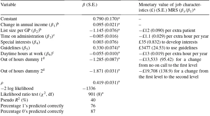
Results for the random effects probit model are shown in Table 3. The sample size was 3255 observations and 773 GPs, after the deletion of missing values for the dependent variable. All coefficients were statistically significant, except special interests and hours of administration. These, therefore, had no effect on the choice of practice. The signs of coefficients were all of the expected direction, except that for guidelines. The signs reflect the effect of a change in the attribute on utility. It appears that GPs preferred a practice that used guidelines, had a lower list size, had a lower number of daytime hours worked per week, offered a higher change in income, and had a lower out of hours workload. These broadly confirm the theoretical validity of the technique. In particular, GPs’ utility was increasing in income, and decreasing with time spent at work.
The positive and significant constant in the model suggests either that GPs were consid-ering attributes not in the model, or that there was ‘right’ bias, where GPs were more likely to favour ‘Practice B’. This may also be due to the existence of a constant scenario. The
value ofρ,measuring the correlation between responses from the same GP, is statistically
significant suggesting that a random effects specification was appropriate and there were unobserved interactions between GP characteristics and attributes.
Table 3
Regression results
Variable β(S.E.) Monetary value of job
character-istics (£) (S.E.) MRS (βx/β1)a
Constant 0.790 (0.170)∗ –
Change in annual income (β1)b 0.095 (0.021)∗ –
List size per GP (β2)b −1.145 (0.076)∗
−£12 (0.090) per extra patient Time on administration (β3)c −0.005 (0.016) −£1.1 (0.029) per extra hour per year Special interests (β4) 0.003 (0.076) £35 (0.832) to develop interests
Guidelines (β5) 0.330 (0.074)∗ £3477 (24.53) to use guidelines
Daytime hours at work (β6)c −0.055 (0.010)∗
−£13 (0.019) per extra hour per year Out of hours dummy 1d −1.285 (0.087)∗
−£13,533 (95.42) for a change from no on call to the first level Out of hours dummy 2d −1.871 (0.031)∗ −£19,708 (138.9) for a change from
the first level to the second level
ρ 0.419 (0.031)∗
aStandard errors for the monetary valuations were calculated from a Taylor series approximation to the variance
of a function of random variables (see Propper, 1995; Kmenta, 1986, p. 486).
bThe independent variables for income and list size were scaled down by a factor of 1000 before analysis, and
re-scaled to calculate monetary valuations.
cSince these variables were hours per week, MRS was divided by 46.5 working weeks per year to reflect the
value of one extra hour per year.
dOut of hours care were coded as two dummy variables. The first reflects the marginal valuation of a change
from no out of hours care to the first level. The second reflects the marginal valuation of a change from the first to the second level. A third situation of no change was used as the omitted dummy variable.
∗
P <0.0001.
GPs would be willing to pay (i.e. give up an increase in income) nearly £3500 to work in a practice with guidelines. The use of guidelines was expected to have a negative effect on utility as it was thought to reduce clinical autonomy. Guidelines may not have therefore been valued because of their effect on autonomy, but for their effect on the quality of care. If so, this suggests that GPs are willing to trade-off income to increase quality of care. However, the type of guidelines (evidence-based or internal to the practice based on consensus) was not specified in the questionnaire and GPs may attach different values to different types of guidelines. Furthermore, the existence of guidelines may also reflect concerns about avoiding litigation, which may be related to income and reputation as arguments in the utility function.
The current capitation payment GPs receive for each patient registered with them is £9 (after tax of 40%) for patients under 65, slightly lower than the valuation found in this study (£12).The results of the reduced regression model with interaction terms shows how the marginal valuation of each attribute differed across GP and current practice characteristics (Table 4). For the reduced model, a likelihood ratio test of the joint statistical significance of the excluded variables failed to reject the null hypothesis that the coefficients of
ex-cluded variables were equal to zero (χ2 = 22 (74 df);P > 0.05), thus favouring the
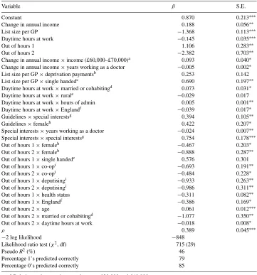
restricted model. In the reduced model, guidelines, special interests and hours of admin-istration drop out of the model, and therefore had no influence on the choice of practice once differences in GP and practice characteristics were accounted for. However, guide-lines and special interests do appear in the interaction terms, indicating that they were important only for a sub-group of GPs. Monetary valuations for the specific sub-groups of GPs are shown in Table 5. The monetary valuations for sub-groups of GPs indicate the relative strength of preference and provide an indication of how much GPs would be willing to pay (or willing to accept) to work in a practice with a specific job charac-teristic.
GPs with total annual after-tax incomes between £60,000 and £70,000 placed a higher value on each extra pound, compared to those earning between £20,000 and £40,000. It would be expected (generally) that people on low incomes value an extra pound more highly than people on high incomes. However, it is just as plausible that GPs earning above a certain amount find income very important to them, compared to GPs who earn less and perhaps place a higher value on non-pecuniary job characteristics.
The more time GPs had spent working as a doctor, then the lower the value placed on each extra pound increase in income. GPs who were single handed or who received deprivation payments for at least 10% of their patients were more likely to prefer a practice with a higher list size, compared to GPs in group practice or GPs not in receipt of deprivation payments, respectively. Deprivation payments are an extra source of income.
GPs who were married or cohabiting preferred more hours at work during the day, compared to other GPs. Those who were in England or who received rural practice payments preferred fewer hours at work, thus placing a higher value on leisure time. However, GPs who spent more time on administration were more likely to prefer a practice with longer working hours per week, although this may reflect a selection effect.
Those GPs who had a special interest were more likely to value a practice that used guidelines, compared to GPs who did not have a special interest. This was also the case for female GPs. For those with special interests, this may reflect increased knowledge about specific clinical areas and an appreciation of the value of information on how to manage certain illnesses. They may therefore regard general practices that use guidelines as having a higher quality of care provided to patients.
Table 4
Regression results for model with interaction terms (reduced model)
Variable β S.E.
Constant 0.870 0.213∗∗∗
Change in annual income 0.188 0.056∗∗
List size per GP −1.368 0.113∗∗∗
Daytime hours at work −0.145 0.035∗∗∗
Out of hours 1 1.106 0.283∗∗
Out of hours 2 −2.382 0.703∗∗
Change in annual income×income (£60,000–£70,000)a 0.093 0.040∗
Change in annual income×years working as a doctor −0.005 0.002∗
List size per GP×deprivation paymentsb 0.253 0.142
List size per GP×single handedc 0.690 0.197∗∗
Daytime hours at work×married or cohabitingd 0.073 0.031∗
Daytime hours at work×rurale −0.029 0.017
Daytime hours at work×hours of admin 0.005 0.001∗∗
Daytime hours at work×Englandf −0.039 0.017∗
Guidelines×special interestsg 0.394 0.105∗∗
Guidelines×femaleh 0.422 0.207∗
Special interests×years working as a doctor −0.024 0.007∗∗
Special interests×special interestsg 0.754 0.178∗∗∗
Out of hours 1×femaleh −0.467 0.203∗
Out of hours 2×femaleh −0.888 0.287∗∗
Out of hours 1×single handedc 0.576 0.301
Out of hours 1×co-opi −0.693 0.191∗∗
Out of hours 2×married or cohabitingd −1.077 0.350∗∗
Out of hours 2×daytime hours at work −0.018 0.008∗
ρ 0.389 0.045∗∗∗
−2 log likelihood −848
Likelihood ratio test (χ2, df) 715 (29)
PseudoR2(%) 46
Percentage 1’s predicted correctly 79
Percentage 0’s predicted correctly 85
aRelative to those on incomes between £20,000 and £40,000.
bRelative to GPs not in receipt of deprivation payments for at least 10% of their patients. cRelative to GPs in group practice.
dRelative to those who are single, separated, divorced or widowed. eRelative to GPs who do not receive rural practice payments. fRelative to GPs in Scotland.
gRelative to GPs with no special interests. hRelative to males.
iRelative to GPs who are single-handed or in a rota.
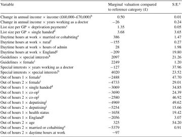
Table 5
The effect of GP and practice characteristics on monetary valuations
Variable Marginal valuation compared
to reference category (£)
S.E.a
Change in annual income×income (£60,000–£70,000)b 0.50 0.01
Change in annual income×years working as a doctor −26 0.24
List size per GP×deprivation paymentsc 1.35 0.05
List size per GP×single handedd 3.68 3.65
Daytime hours at work×married or cohabitinge 386 1.47
Daytime hours at work×ruralf −155 0.27
Daytime hours at work×hours of admin 28 1.98
Daytime hours at work×Englandg −209 19.80
Guidelines×special interestsh 2097 21.26
Guidelines×femalei 2249 1.20
Special interests×years working as a doctor −127 37.96
Special interests×special interestsh 4020 23.52
Out of hours 1×femalei −2488 47.70
Out of hours 2×femalei −4733 29.01
Out of hours 1×single handedd −3069 34.85
Out of hours 1×co-opj −3690 24.39
Out of hours 2×co-opj −2580 46.92
Out of hours 1×deputisingj −4969 49.62
Out of hours 2×deputisingj −5254 15.66
Out of hours 1×health status −1658 19.42
Out of hours 1×Englandg −2056 3.07
Out of hours 2×age 325 54.20
Out of hours 2×married or cohabitinge −5379 0.91
Out of hours 2×daytime hours at work −97
aStandard errors for the monetary valuations were calculated from a Taylor series approximation to the variance
of a function of random variables (see Propper, 1995; Kmenta, 1986, p. 486). These can be used to test whether the valuations are significantly different from zero.
bRelative to those on incomes between £20,000 and £40,000.
cRelative to GPs not in receipt of deprivation payments for at least 10% of their patients. dRelative to GPs in group practice.
eRelative to those who are single, separated, divorced or widowed. fRelative to GPs who do not receive rural practice payments. gRelative to GPs in Scotland.
hRelative to GPs with no special interests. iRelative to males.
jRelative to GPs who are single-handed or in a rota.
The marginal valuation of the amount of out of hours workload was influenced by a number of GP characteristics. GPs in Scotland and GPs in poorer health were more likely to prefer a change from no out of hours work to doing some out of hours work (level 1), compared to GPs in England and those in better health, respectively. Older GPs were more likely to prefer an increase in the amount of out of hours work from the first to the second level, compared to younger GPs.
(again reflecting selection effects), those who were married or cohabiting, and those working longer hours during the day.
Some sub-groups of GPs had preferences for more than one job characteristic. Female GPs preferred a practice with guidelines and less out of hours care. GPs who were mar-ried or cohabiting preferred to work more during the day and less at night. GPs who had been working longer as doctors were less likely to prefer a practice with special inter-ests or with an increase in income. Single-handed GPs were more likely to prefer a prac-tice with a higher list size and where they did not have to undertake any out of hours work. GPs in England preferred a practice with fewer hours at work during the day and night.
5. Discussion
This study has examined the preferences of GPs for the characteristics of their job, re-vealed through the choice of a practice in which to work. In this particular choice context, the results suggest that non-pecuniary job characteristics, particularly out of hours care, in-fluence practice choice. Workload (proxied by list size), daytime hours at work, income and the practice’s use of guidelines were also statistically significant determinants. Time spent on administration and opportunities to develop special interests (a proxy for intellectual satisfaction) were significant for some sub-groups of GPs.
The results suggest that preferences differed across sub-groups of GPs, and that they would require different policies to influence their choice of practice. For certain sub-groups, there is also evidence that preferences are related to GPs’ current situation, e.g. GPs who currently use deputising services are less likely to prefer out of hours work. This suggests that their stated preferences are reflected in their current choices.
GPs obtained positive utility from certain job characteristics, especially from the use of guidelines, special interests if the GP already has special interests, daytime hours at work if the GP is married or cohabiting (but disutility from out of hours work if married or cohabiting), list size if the GP is single handed or receives deprivation payments, and from out of hours care if the GP is older.
The results should be interpreted with the following caveats. First, the model assumed that other job characteristics are constant across practices in the choice set. In answers to open-ended questions, good working relationships with partners was found to be potentially more influential than characteristics included in the model, when choosing a practice in which to work. Thus, if ‘good working relationships’ differs across practices in the choice set, any financial incentive suggested by our results may not be effective for some GPs. Factors that were not amenable to policy influence were not included (e.g. good working relationships and local area characteristics).
of ‘dominance’ for specific attributes, suggesting that individuals are not using compen-satory decision rules. This may be because of the complexity of the questionnaire (bounded rationality) or because they genuinely have a dominant preference (Drakopoulos, 1994; Scott, 1998). This study did not examine this issue since it was felt that presenting GPs with only four discrete choices did not provide enough information on which to conclu-sively state that a GP who always chose the option with the ‘best level’ had a dominant preference.
Nevertheless, the existence of dominant preferences may explain the very high values for out of hours work. It should be noted that when ranking the attributes, 52% of respondents ranked out of hours care as the most important. This can be regarded as an indication of
the maximum proportion of respondents with apotentiallydominant preference for out of
hours care. These GPs may have always been selecting the option with the lowest level of out of hours commitment, and ignoring other attributes. If so, then doubt must be expressed about the monetary valuations as they may overestimate the strength of preference for those who were willing to trade. Using the valuation to argue that GPs should be paid £13,500 to undertake out of hours work may therefore be misleading. Some GPs, if they have a
lexicographic preference, may not be prepared to acceptanymonetary amount to undertake
such work. This also applies to other characteristics. However, it is not unreasonable to expect that when choosing a practice in which to work, that GPs may trade-off increases in income to have better quantities of other attributes.
The theoretical validity of the technique is confirmed, with a positive marginal utility of income, and negative marginal utility of time at work. One questionnaire had a check for internal consistency, and only one GP out of 188 was inconsistent. Many other discrete choice experiments have reported high levels of internal consistency. One study has ex-amined the convergent validity of conjoint analysis, by comparing it with usual hedonic methods. This found that the value of risk was not significantly different between the two approaches, and suggested that conjoint analysis may be superior in assessing the marginal valuation of safety (Gegax and Stanley, 1997).
The policy conclusions from this study relate to the locational choices of GPs, and policies aimed at reducing inequalities in the distribution of GPs. In the UK, current decisions on GP distribution are made by the Medical Practice Committee in England and Scotland. However, these decisions relate to the power to say ‘yes’ or ‘no’ to new GP practices being set up. Individual health authorities can use financial incentives through the National GP Contract (e.g. through inducement payments). Changes to the financing and organisation of out of hours care in 1995 have meant that GPs’ out of hours commitments have been considerably reduced, especially in urban areas. The effect of these policies on GPs’ location choices and inequality in distribution is, however, unclear. Additional policies could be introduced to be able to alter non-pecuniary job characteristics with the aim of influencing location choices into underserved areas. Furthermore, the analysis here does not take into account the transactions costs of switching jobs for GPs.
Acknowledgements
This study was funded by a grant from the Scientific Foundation Board of the Royal College of General Practitioners (RCGP). Thanks to John Cairns, Bob Hart, Carol Propper and two anonymous referees for comments. The Health Economics Research Unit is funded by the Chief Scientist Office of the Scottish Executive Health Department (SEHD). The views in this paper are those of the author and not RCGP or SEHD.
References
Arai, M., 1994. Compensating wage differentials versus efficiency wages: an empirical study of job autonomy and wages. Industrial Relations 33, 249–262.
Beardow, R., Cheung, K., Styles, W.M., 1993. Factors influencing the career choices of general practitioner trainees in North West Thames Regional Health Authority. British Journal of General Practice 143, 449–452. Cavalluzzo, L.C., 1991. Non-pecuniary rewards in the workplace: demand estimates using quasi-market data.
Review of Economics and Statistics 73, 508–512.
Chakraborty, G., Gaeth, G.J., Cunningham, M., 1993. Understanding consumers’ preferences for dental service. Journal of Health Care Marketing 21, 48–58.
Department of Health, 1994. General Medical Practitioners’ workload survey 1992–1993. Joint Evidence to the Doctors’ and Dentists’ Review Body from the Health Departments and the GMSC.
Dionne, G., Contandriopoulos, A., 1985. Doctors and their workshops: a review article. Journal of Health Economics 4, 21–33.
Drakopoulos, S.A., 1994. Hierarchical choice in economics. Journal of Economic Surveys 8, 133–153. Ehrenberg, R.G., Smith, R.S., 1988. Modern Labour Economics: Theory and Public Policy, 3rd Edition. Scott,
Foresman and Company, Illinois.
Electoral Ballot Reform Services, 1992. Your choices for the future: a survey of GP opinion, General Medical Services Committee.
Encinosa, W.E., Gaynor, M., Rebitzer, J.B., 1997. The sociology of groups and the economics of incentives: theory and evidence on compensation systems. Working Paper 5953, National Bureau of Economic Research. Evans, R.G., 1974. Supplier-induced demand: some empirical evidence and implications. In: Perlman, M. (Ed.),
The Economics of Health and Medical Care. International Economics Association, Macmillan, New York. Feldstein, M., 1970. The rising price of physicians’ services. Review of Economics and Statistics 52, 121–133. Fowkes, T., Wardman, M., 1988. The design of stated preference travel choice experiments. Journal of Transport
Economics and Policy 22, 27–44.
Gegax, D., Stanley, L.R., 1997. Validating conjoint and hedonic preference measures: evidence from valuing reductions in risk. Quarterly Journal of Business Economics 36, 31–54.
Gronberg, T.J., Reed, W.R., 1994. Estimating workers marginal willingness to pay for job attributes using duration data. Journal of Human Resources 29, 911–931.
Herzog, H.W., Schlottmann, A.M., 1990. Valuing risk in the workplace: market price, willingness to pay and the optimal provision of safety. Review of Economics and Statistics 72, 463–470.
Kmenta, J., 1986. Elements of Econometrics, 2nd edition. Macmillan, New York.
Kniesner, T.J., Leeth, J.D., 1991. Compensating wage differentials for fatal injury risk in Australia, Japan, and the United States. Journal of Risk and Uncertainty 4, 75–90.
Kristiansen, I.S., 1994. What is in the doctor’s utility function? A theoretical and empirical investigation into what influences doctors’ decision making. Ph.D. Thesis, University of Tromso.
Manski, C.F., 1977. The structure of random utility models. Theory and Decision 8, 229–254.
McFadden, D., 1974a. The measurement of urban travel demand. Journal of Public Economics 3, 303–328. McFadden, D., 1974b. Conditional logit analysis of qualitative choice behaviour. In: Zarembka, P. (Ed.), Frontiers
in Econometrics. Academic Press, New York.
Permain, D., Swanson, J., Kroes, E., Bradley, M., 1991. Stated Preferences Techniques: A Guide to Practice, 2nd. Edition. Steer Davis Gleave and Hague Consulting Group.
Propper, C., 1995. The disutility of time spent on UK National Health Service waiting lists, Journal of Human Resources 30(4).
Roswell, R., Morgan, M., Sarangi, J., 1995. General practitioner registrars’ views about a career in general practice. British Journal of General Practice 45, 601–604.
Rottenberg, S., 1971. On choice in labour markets. In: Burton, J.F., Benham, L.K., Vaughn, W.M., Flanagan, R.J. (Eds.), Readings in Labour Market Analysis. Holt, Rinehart and Winston Inc, New York.
Sandy, R., Elliott, R.F., 1998. Adam Smith was right after all: another look at compensating differentials. Economic Letters 59, 127–131.
Scott, A., 1997. Designing incentives for GPs. A review of the literature on their preferences for pecuniary and non-pecuniary job characteristics. Discussion Paper 01/97, Health Economics Research Unit, University of Aberdeen.
Scott, A., 1998. Giving things up to have more of others. The implications of limited substitutability in eliciting preferences for health and health care. Discussion Paper 01/98, Health Economics Research Unit, University of Aberdeen.
Scott, A., 2000. Agency and incentives in general practice. Ph.D. Thesis, University of Aberdeen.
Small, K.A., Rosen, H.S., 1981. Applied welfare economics with discrete choice models. Econometrica 49, 105– 130.
Stewart, M.A., 1995. Effective physician communication and health outcomes: a review. Canadian Medical Association Journal 152, 1423–1433.
Truong, T.P., Hensher, D.A., 1985. Measurement of travel time values and opportunity cost from a discrete choice model. The Economic Journal 95, 438–451.
Vick, S., Scott, A., 1998. Agency in health care. Examining patients’ preferences for attributes of the doctor-patient relationship. Journal of Health Economics 17, 587–606.
Wardman, M., 1998. The value of time: a review of British evidence. Journal of Transport Economics and Policy 32, 285–315.