M02149

(1)

Proceedings of

4

TH

INTERNATIONAL CONFERENCE

(2)

ii

PREFACE

The Fourth International Conference on Mathematics and Statistics is an annual program

belong to MSMSSEA (Muslim Statisticians and Mathematicians Society in South East

Asia) in collaboration with Institute Statistics of Malaysia (ISM), Persatuan Matematik

Malaysia (PERSAMA), Indonesia Mathematics Society (Indo MS), Universitas

Malahayati, and Universiti Malaysia Terengganu.

The Participants of the conference are about 100 coming from more than 20 higher

institutions, among others Universitas Gadjah Mada (UGM), Institut Teknologi Bandung

(ITB), Universitas Indonesia (UI), Institut Pertanian Bogor (IPB), Universitas Putra

Malaysia (UPM), Institut Teknologi Sepuluh Nopember (ITS), Universitas Kebangsaan

Malaysia, Waseda University Japan, Chinese Academy of Science Sanghai China,

University of Twente Netherland, Nasional University of Malaysia, International Islamic

University Malaysia, Universitas Guna Darma, Universiti Islam Antar Bangsa Malaysia,

Universitas Sriwijaya, Lembaga Sandi Negara.

I hope this conference will be a big class for professor in Mathematics and Statistics and

their students to exchange ideas and share of knowledge and experience. This kind of

conference will surely have a positive impact on higher education in general as well as

in the development of mathematics and statistics and its applications. In addition the

conference will encourage the faculty members to do more and more research.

On behalf of the Steering Committe, we would like to express our deepest gratitude to

the Foundation of Alih Teknologi, Rector Universitas Malahayati, International advisory

Board Members, and to all participants we are also grateful to all organizing committee

members and all the reviewers, without those efforts such a high standard for the

conference could not have been achieved.

Bandarlampung, 11 August 2009

(3)

iii

PROCEEDINGS

4

TH

INTERNATIONAL CONFERENCE ON MATHEMATICS AND

STATISTICS (ICOMS 2009)

UNIVERSITAS MALAHAYATI BANDARLAMPUNG

on August, 13-15

th

2009

Editor in Chief:

Ismail Bin Mohd

Faculty of Engineering University Malaysia Terengganu

Editor Assistant:

Iing Lukman

Faculty of Economic, Universitas Malahayati, Indonesia

Editors:

1.

Noor Akma Ibrahim

Department of Mathematics/

Institute for Mathematical Research,

Universiti Putra Malaysia

2.

Iing Lukman

Faculty of Economics,Universitas

Malahayati Bandar Lampung,

Indonesia

3.

Maman A. Djauhari

Department of Mathematics and a

Sciences, Institut Teknologi

Bandung (ITB), Indonesia

4.

Ismail Bin Mohd

Department of Mathematics,

Universitas Malaysia Terengganu

(UMT), Malaysia

5.

Abdul Kudus

Department of Statistics, Universitas

Islam Bandung (Unisba), Indonesia

6.

Mustofa Usman

Faculty of Mathematics and

Sciences, Universitas Lampung,

Indonesia

7.

Agung Efriyo Hadi

Faculty of Engineering, Universitas

Malahayati Bandar Lampung,

Indonesia

8.

Wamiliana

Faculty Of Mathematics and

Sciences, Universitas Lampung,

Indonesia

9.

Muhammad Rizam Bin Abu Bakar

Department of Mathematics,

Universiti Putra Malaysia (UPM)

Malaysia

10.

Faiz A.M Elfaki

Department of Sciences, Faculty of

Engineering, International Islamic

University Malaysia, Malaysia

11.

Mustofa Mamat

Head of Department of Mathematics

Universiti Malaysia Terengganu.

12.

Admi Syarief

(4)

4

TH

INTERNATIONAL CONFERENCE ON MATHEMATICS AND

STATISTICS (ICOMS 2009)

UNIVERSITAS MALAHAYATI BANDARLAMPUNG

© MSMSSEA AND UNIVERSITAS MALAHAYATI 2009

on August, 13-15

th

2009

Organizing Commmitee

Chair Person

: Iing Lukman, Ph.D

Vice Chair Person

: Dr. Ir. Hardoyo Marsyad, M. Eng

Secretary

: Indah Lia Puspita, S.E.,M.Si

Treasurer

: Devi Oktarina, M.T

Special Events

: Weka Indra Dharmawan, M.T

1. Agustina Retnaningsih, Apt

2. Rina Febrina, S.T

3. H. Drs. Djamaludin H.S

4. Anita K, S.E., M.Com (Acc)

Secretariat

: Eka Sariningsih, S.E

1.

Natalina, S.T

2.

Ade Maria Ulfa, S. Farm

Facility and Decoration

: Tumpal OR, S.T

1.

Muhammad Luthfi, S.E

2.

Heri Wibowo, S.T

3.

Iskandar Muda, S.H

4.

Hasan Saputra

5.

Abu Rohmat, S.E

6.

Aminullah, S.E

7.

Adi Wijoyo

Consumption

: Erna Listyaningsih, S.E.,M.Si

1.

Lestari Wuryanti, S.E

2.

Hardini Ariningrum, S.E

3.

Emy Khikmawati, S.T

4.

Dra. Hj. Sulastri, MTA

Transportation and Accomodation : Widianto, S.T

1.

Ir. Yanjuansyah, DEA

2.

Robby Chandra, S. Farm

Documentation and Publication

: Fredi Setiawan, S.T

(5)

DETERMINATION PARAMETER BY NONLINEAR LEAST SQUARE

H.A Parhusip

1

1_{Department of Industrial Mathematics and Statistics,}

Faculty of Science and Mathematics , Satya Wacana Christian University, Indonesia

_________________________________________________________________________

Abstract.

Determination parameter from the given data by nonlinear least square is discussed here. The case study is expressing Salatiga’s income as a function of tax and retribution using calculus multivari-able. The function is then used in the system of ordinary differential equation. Its equilibrium point is obtained by using trust region algorithm since the equilibrium is the solution of the governing nonlinear system. The solutions of nonlinear ordinary differential equations are also presented.

Keywords : nonlinear least square, nonlinear equations, equilibrium points.

1.

Introduction

This research is motivated by a limitation of knowledge in many branches of mathematics for undergraduate. On the other hand, students face various data from the small companies and government in their surroundings. With some branches in mathematics, students have difficulties to integrate their knowledge to the given data and one has to analyze data with various interests. Therefore this paper pro-vides the basic idea on this direction.

Frequently, determination of parameters leads to solving nonlinear system such that the chosen function fit to the given data especially in the case of nonlinear system. Motor parameter determination for transient torque calculations for example, Pragasen, et.all [1997] applied genetic algorithms and com-pared to Newton-Raphson method.

On this paper we present that the function has two variables and its parameters determined by nonlinear least square as shown by Stoer and Bulirsch [1991] whereby we try to minimize the average square deviation of the approximating function on a set of selected points. Since data are multivariable, one may use multivariate calculus and choose a certain function. We expect the function has special properties such as an existence of minimizer, boundedness, continuity and differentiability in the given domain of definition. The minimization problem reduces into a problem of solving nonlinear system. Therefore one has to choose an available algorithm to solve the system. Some algorithms are available in software packages such as MATLAB. However difficulties may appear to make a good initial guess to use an available algorithm.

Salatiga is one of the small cities in Central Java, Indonesia. There are some sectors provide the income to the Department of Financial in Salatiga (Dinas Pengelolaan Keuangan Daerah Salatiga). The case study is an analysis of the income as a function of city’s tax and retribution given by society. We assume that other sectors are not significant.

This paper is organized as follows. Derivation of Salatiga’s income as a function of tax and ret-ribution and a competition model are presented in Section 2. Procedures to develop the models and theirs solutions are shown in Section 3. Finally, the Section 4 shows the result and the Conclusion is stated in the Section 5.

II.1 Salatiga’s income as a function of tax and retribution

In this section the theory is introduced by assuming that the income as a function of tax and retri-bution. We introduce the symbols

1

x

:=the tax every month,

x

₂:= the retribution every month

(6)

f

(

x

₁,

x

₂) =

f

(

x, β)

=

β

₁

x

₁

x

₂

+

β

₂

x

₂ (1) with

β

₁and

β

₂ must be known from the data. We will find the parameters in the function by presenting the data Table 1 into dimensionless. This is done by introducing the new variables

) max( 1 1 1 x x x = ;

)

max(

₂ 2 2

x

=

;

(

)

(

1 2

)

2 1 , max ) , ( x x y x x y

y= ;

)) , ( max( ) , ( 2 1 2 1 x x f x x f

W = . (2)

Table 1. Salatiga’s income in four months(unit : Rupiah)

1

x

_{134 058 621} _{941 207 840 1 401 847 464 1 891 305 201}

2

x

_{844 319 263 1 811 186 084 3 095 003 843 4 350 541 386}

y 978 377 884 978 377 884 4 496 851 307 6 241 846 587

Formulation data into dimensionless is not unique but the given rule in the equation (2) is the simplest one. Using equation (2) we may rewrite the data into dimensionless and list the data in the Table 2.

Table 2. Data Table 1 in dimensionless

1

ˆx

0.0709 0.4976 0.7412 1.000

2

ˆx

_{0.1941 0.4163} _0.7114 _1.000

y

_{0.1567 0.4410} _0.7204 _1.000

The values of

β

₁and

β

₂ can be estimated by weighted nonlinear least square (Stoer and Bulirsch 1993) that is

minimize

[

]

[

₁ ₁() ₂() ₂ ₂()

]

2

1 2 1

)

(

ˆ

i i i

i m i i m i i i

i

y

W

w

y

x

w

Q

=

∑

−

=

∑

−

β

+

β

= =

and m = 4. (3)

We have to minimize the quadratic sum that means the condition



=











∂

≡

∇

T

Q

2 1

,

β

0 must be

sat-isfied. We get

=

∂

1

β

Q

[

]

(

)

0

)

(

ˆ

2

2()

) ( 1 ) ( 2 2 ) ( 2 ) ( 1 1 1

=

−

+

−

∑

= i i i i i i m i

i

y

x

w

β

(4a)

=

∂

2

β

Q

[

]

(

)

0

)

(

ˆ

2

₁ ₁() ₂() ₂ ₂() ₂()

1

=

−

+

−

∑

= i i i i i m i

i

y

x

w

β

. (4b)

The equation (4a)-(4b) can be rewritten as a linear system for

β

₁ and

β

₂ that is

( )

[ ] [ ]

[ ][ ]

( )

[ ]

[ ][ ]

( ) () 2 1 1 2 ) ( 2 1 1 2 2 ) ( 2 2 1 1 1

ˆ

i i m i i i i i m i i i i m i

i

x

w

x

w

y

x

w

∑

= = =

=

+

β

(5a)

( )

[ ][ ]

[ ]

() 2 1 2 ) ( 2 1 2 2 ) ( 2 1 1 1

ˆ

i m i i i i m i i i i m i

i

x

w

x

w

y

x

w

∑

= = =

=

+

β

(7)

The equations (5a-5b) contain the unknown

w

_i. Therefore we assume that

w

_i=1. This means that we are going back to the standard least square method to get

( )

[ ] [ ]

[ ][ ]

( )

[ ]

[ ][ ]

( ) () 2 1 1 2 ) ( 2 1 1 2 2 ) ( 2 2

1 1

1

ˆ

i i m

i i i

i m

i i

i m

i

x

y

x

∑

= =

=

+

β

(6a)

( )

[ ][ ]

[ ]

()

2 1 2 ) ( 2 1 2 2 ) ( 2 1 1

1

ˆ

i m

i i i

m

i i

i m

i

x

y

x

∑

= =

=

+

β

. (6b)

By solving the equations (6a)-(6b) we obtain

β

₁ = 0.0180 dan

β

₂ = 0.9902 therefore

2 2

1

0

.

9902

0180

.

0

x

f

=

+

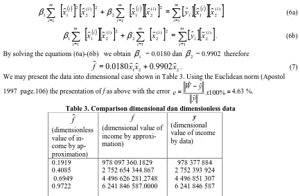
. (7)

We may present the data into dimensional case shown in Table 3. Using the Euclidean norm (Apostol

1997 page.106) the presentation of f as above with the error ₌ − ₁₀₀_%₌ ˆ

ˆ

x y

y W

e 4.63 %.

Table 3. Comparison dimensional dan dimensionless data

f

(dimensionless value of in-come by ap-proximation)

f

(dimensional value of income by approxi-mation)

y

(dimensional value of income by data)

0.1919 0.4085 0.6949 0.9722

978 097 360.1829 2 752 654 344.867 4 496 626 281.2748 6 241 846 587.0000

978 377 884 2 752 393 924 4 496 851 307 6 241 846 587

In the next following sections we remove the sign ‘tilde’ though the variables contain no dimensions for simplicity.

II.2 Competition model between two sectors

Since there are two sectors that contribute to maximize the income therefore we assume there will be a competition between two sectors. We use a competition between two sectors as a competition model (Stewart [1999]). Using t to denote time we have the system of ordinary differential equations as

2 1 1 1 1

1

x

dt

dx

=

α

−

β

(8a)

2 1 2 2 2 2

x

dt

dx

=

α

−

β

(8b)

(8)

0

1

=

dt

dx

2

=

0

dt

dx

. (9)

The point

(

x

₁

*,

x

₂

*)

that satisfies equation (9) is called an equilibrium point. This means that we seek the solution of

α

₁

x

₁

−

β

₁

x

₁

x

₂

=

0

and

α

₂

x

₂

−

β

₂

x

₁

x

₂

=

0

.

We have the equilibrium points

are (0 0) and













2 2 1 1

,

β

α

β

α

. The point (0 0) has no practical used because it is only trivial solution. The

sec-ond equilibrium point shows the ratio between the weight of each sector and its interaction with the other sector.

The values of parameter are obtained by assuming that initially each sector grows exponentially

and therefore we have exponential models for both dependent variables. These

are

x

(

₀

)

e

1t

1 1

α

=

dan

x

(

₀

)

e

2t

2 2

α

=

with

x

₁

(

0

)

and

x

₂

(

0

)

indicate the initial values of both sectors. Using the logarithm function on both functions and linear regressian (Parhusip [2008]) we obtain that the value of parameters are

α

₁=0.0159 dan

α

₂=0.0104. The values of

β

₁and

β

₂can be obtained by assum-ing

β

₁=1-

α

₁and

β

₂=1-

α

₂. Again one may choose freely the model of parameters but we try to minimize difficulties to design the model. Finally we will integrate both approaches in the sections II.1 and II.2 in the next section.

II.3 Modelling of the competition model between two sectors

In the section II.1 we have an expression of interaction of both sectors (tax and retribution). By comparing the equations (7) dan (8b) we have derived

2 1 2 2 1 2 2

0180

.

0

9902

.

0

)

,

(

x

g

dt

dx

=

−

.

Similarly we may construct

2 1 1 1 1 2 1 1 1

)

,

(

x

g

dt

dx

β

α

−

=

.

We apply nonlinear weighted least square to determine the parameters. This means that we have to solve













=

























∑

= = = = = = N i i i i i N i i i i N i i i i N i i i i N i i i N i i i

x

y

w

x

y

w

x

w

x

w

x

w

1 , 2 , 1 1 , 1 1 1 1 2 , 2 2 , 1 1 , 2 2 , 1 1 , 2 2 , 1 1 2 , 1

β

α

(10a)

(9)













=

























∑

= = = = = = N i i i i N i i i N i i i N i i i N i i i N i i

x

y

x

y

x

1 , 2 , 1 1 , 1 1 1 1 2 , 2 2 , 1 1 , 2 2 , 1 1 , 2 2 , 1 1 2 , 1

β

α

. (10b).

By solving the linear system of equation (10b) we have

α

₁

=

0

.

8810

dan

β

₁

=

0

.

1184

. The system of ordinary differential equations becomes

2 1 1

1

₀

.

8810

x

₀

.

1184

x

dt

dx

=

−

2 1 2 2

0180

.

0

9902

.

0

x

dt

dx

−

=

.

The equilibrium point is given by (0, 0) due to the equation (9).

One has to modify the model such that the model is reasonable and meaningful. Finding the equilibrium solutions to a system of ordinary differential equations is only half of the battle, one must then understand their stability properties in order to characterize those that can be realized in normal physical circumstances. We will use this approach for larger number of data. This is shown in section IV. The type of equilibria in the linear case in general is classified into three groups as mentioned by Golubitsky and Dellnitz, [1999]. These are :center , stable and unstable. One could also consider monotonicity properties.

In the nonlinear case and higher dimensional , we may introduce the linearization technique that can be applied to analyze the stability of an equilibrium

x

*first order autonomous system

)

(x

F

x

=

. (10c).

The linearization is based on approximation of the function

F

(x

)

near an equilibrium point, where

0

)

(

*

=

x

F

by its first order Taylor polynomial

)

)(

(

'

)

)(

(

'

)

(

)

(

* * * * *

x

F

x

F

x

F

x

F

≈

+

−

=

−

(10d)

where

'

(

*

)

x

F

denotes its n x n Jacobian matrix at the equilibrium. Nearby the solutions, we expect that the deviation from equilibrium, say

v

(

t

)

=

x

−

x

*will be governed by linear system

v

A

dt

v

d

=

where

'

(

*

)

x

F

A

=

. (10e)

(10)

Teorema 1. Let

x

*be an equilibrium point for the first order ordinary differential equations

x

=

F

(x

)

. If all the eigenvalues of the Jacobian matrix

F

'

(

x

*

)

have negative real part, then

x

*is asymptotically stable. If, on the other hand,

F

'

(

x

*

)

has one or more eigenvalues with positive real part, then

x

*is un-stable equilibrium.

The borderline case occurs when one or more of the eigenvalues of

F

'

(

x

*

)

is either 0 or purely imaginary, while all eigenvalues have negative real part. In such situations, the linearized stability test is inclusive and we need more detail information to determine the type of stability.

III. Research Method

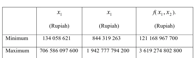
The studied data is taken from the Department of Salatiga’s income in the period January 2005- May 2008. The data is transformed into dimensionless by following section 2. Table 1 shows the range value of

x

₁

,

x

₂ and f(

x

₁

,

x

₂).

Table 1. Data tax

(

x

₁

)

and retribution

(

x

₂

)

1

x

(Rupiah)

1

x

(Rupiah)

f(

x

₁

,

x

₂). (Rupiah)

Minimum 134 058 621 844 319 263 121 168 967 700

Maximum 706 586 097 600 1 942 777 794 200 3 619 274 802 800

After data are dimensionless we may set up the model and seek its parameters based on the given data. The research method is designed mainly to build the mathematical model as follows :

1. Construct the Salatiga’s income as a function of two variables.

2. Formulate the system of ordinary differential equations as a modified competition model.

3. Compute the equilibrium of the governing system by trust region algorithm and analyze the re-sult.

4. Linearized the nonlinear system around the equilibrium point.

5. Determine the type of stability.

(11)

4.1 Salatiga’s income as a function of

x

₁

(

t

)

(tax) and

x

₂

(

t

)

(retribution)

The model is started by assuming that

x

₁

(

t

)

and

x

₂

(

t

)

belong to the space E =C(0,1) of con-tinuous functions over interval (0,1) and we define the map w:

Ω

→

R

with

Ω

=

(

0

,

1

)

×

(

0

,

1

)

. We

want to find an optimal approximation (in the least square sense) in the subspace G consisting of continuous functions in the form

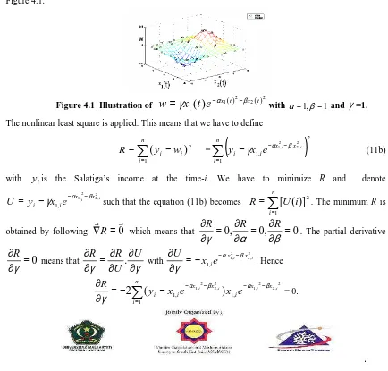
2 2 2 1() () 1

(

)

t x t x

e

t

x

w

=

γ

−α −β . (11a)

The parametet

α

,

β

dan

γ

can be obtained based on the given data. The function is illustrated in the Figure 4.1.

Figure 4.1 Illustration of

2 2 2 1( ) ( ) 1

(

)

t x t x

e

t

x

w

=

γ

−α −β with α=1,β=1 and

γ

=1. The nonlinear least square is applied. This means that we have to define

2 1

)

(

_i n i i

w

y

R

=

∑

−

= =

(

)

2 1 , 1 2 , 2 2 , 1

∑

= − −

−

n i x x i i i i

e

x

y

γ

α β (11b)

with

y

_iis the Salatiga’s income at the time-i. We have to minimize R and denote

2 , 2 2 , 1 , 1 i i x x i

i

x

e

y

U

=

−

γ

−α −β such that the equation (11b) becomes 2

1

]

)

(

[

∑

=

n i

i

U

R

. The minimum R is

obtained by following

∇

R

=

0

which means that

0

,

0

,

=

0

∂

=

∂

=

∂

β

α

γ

R

. The partial derivative

0

=

∂

γ

R

means that

γ

∂

=

∂

U

R

.

with

2 , 2 2 , 1 , 1 i i x x i

e

x

U

α β

γ

− −

−

=

∂

. Hence

∑

= − − − −

−

=

∂

n i x x i x x i i i i i i

e

x

e

x

y

R

1 , 1 , 1 2 , 2 2 , 1 2 , 2 2 , 1

)

(

2

α β α β

(12)

We get

(

)

0

2 1 2 , 1 1 , 1 2 , 2 2 , 1 2 , 2 2 ,

1

−

∑

=

∑

= − − − − = n i x x i x x n i i i i i i

i

x

e

x

y

α β

γ

α β . (12a)

Similarly

=

0

∂

α

R

means that

α

∂

=

∂

U

R

.

with

2 , 2 2 , 1 3 , 1 i i x x i

e

x

U

γ

α β

α

− −

−

=

∂

such that

α

∂

R

=

(

)

0

2 1 4 , 1 2 1 3 , 1 2 , 2 2 , 1 2 , 2 2 ,

1

+

=

−

∑

= − − − − = n i x x i x x n i i i i i i i

e

x

e

x

y

α β

γ

α β

γ

. (12b)

Finally

=

0

∂

β

R

β

∂

=

∂

U

R

.

dan

2 , 2 2 , 1 2 , 2 , 1 i i x x i i

x

e

x

U

γ

α β

β

=

− −

∂

such that

β

∂

R

=

(

)

0

2 1 2 , 2 2 , 1 2 1 2 , 2 , 1 2 , 2 2 , 1 2 , 2 2 ,

1

−

∑

=

∑

= − − − − = n i x x i i x x n i i i i i i i i

e

x

e

x

y

α β

γ

α β

γ

. (12.c)

We may solve the equation (12a)-(12c) using lsqnonlin function provided by MATLAB and we get

0289

.

0

=

α

β

=−0.0202 and

γ

=

1

.

1216

. (13a)

Thus we get

2 2 2

1() 0.0202 ( )

0289 . 0 1

(

)

1216

.

1

x

t

e

x t x t

w

=

− + (13b)

with its error 3.0505%. The small error shows that the given initial guess could lead the expected pa-rameters. Therefore in this case, we need not to find other available algorithms to determine the parame-ters. We may use this result to model the system first order ordinary diferential equations.

4.2 Salatiga’s income as a system of first order ordinary differential equation

Models with system ordinary differential equations are mainly written by literatures such as by Golubitsky and Dellnitz,[1999] where parameters have been defined explicitly. Therefore students have no idea how to design a model with a system ordinary differential equations and its parameters. Section 2 has shown in the linear case. In this section, the modeling of a nonlinear system ordinary differential equations is shown.

Since

2 2 2 1() ()

1

(

)

t x t x

e

t

x

w

=

γ

−α −β as stated in equation (11a) , we may have

(

1

)

1

2

1

2 2 2 1

x

e

x

w

=

γ

αx βx

−

α

∂

− − _and 2

2 2 1 2 1 2

2

x

e

x x

x

w

=

−

γβ

−_α −_β

(13)

to obtain

)

2

1

(

2

)

/

1

(

)

/

1

(

1 2 1 1 2 1 2 2 1 2 2 2 1 3 2 2 1

x

e

x

dt

dx

dt

dx

dt

dx

dt

dx

x

w

x

w

x x x x

α

γ

γβ

β α β α

−

=

∂

− − − − .

By substituting the parameters presented in equation (13a) we have the system ordinary differential equations becomes

(

1

)

0202 . 0 0289 . 0 1

)

0289

.

0

(

2

1

1216

.

1

e

12 22

x

dt

dx

=

− x + x

−

_(14a)

2 2 2

1 0.0202

0289 . 0 2 1 2

0453

.

0

x

e

x x

dt

dx

=

− +

(14b)

The equilibrium point is obtained by solving the solution of nonlinear equations ,i.e 1 =₀

dt

dx _and

0

2 =

dt

dx _{(following (9)). The most popular methods for solving nonlinear system are Newton method}

and its modification (Stoer and Bulirsch [1991]). Some other techniques are trush region, Broyden method and Halley method. The algorithm of global optimization with a constraint bound function as an embedded trust region is explored by Addis and Leyffer [2004]. Grosan and Abraham [2008] stated that one of the new approaches for solving nonlinear systems is rewritten nonlinear system into multiobjective optimization problem. On this paper we use the algorithm trush region provided by MATLAB with the function lsqnonlin.m to get the equilibrium point

(

x

ˆ

₁

*,

x

ˆ

₂

*)

= (14.2059 0.0021). Since the references value are

x

1,Re_f

=

Rp.7 065 860 976 dan

x

2,Ref

=

Rp.19427777942 the dimensional value is

*)

*,

(

x

1

x

2 =(

11

10

0038

.

1

×

4

.

0171

×

10

7

)

. The solutions of the system (14a)-(14b) are shown in

the Figure (4.2a-4.2b). We get the sector

x

₁

(

t

)

grows faster than

x

₂

(

t

)

with positive gradient.

The stability of equilibrium point can be showed by linearized the system and seek its Jacobian in its equilibrium. Following the linearization in Section 2 leads to

(

)

(

)

(

)

(

)













−













−

+

−

=

−

≈

− − * 2 2 * 1 1 2 * 2 * 1 2 * 1 * 2 * 1 * 1 * 1 ) ( ) ( * *

)

(

2

)

(

2

1

2

)

2

1

(

1

2

)

)(

(

'

)

(

2 * 2 2 * 1

x

e

x

F

x

F

x x

β

γβ

α

γβ

α

γβ

α

αγ

β α

Substitute the parameters and equilibrium point , we get .

)

(x

F

=













−













−

0

.

0021

(14)

The Jacobian matrix

F

'

(

x

*

)

has eigenvalues -0.0007 and 0.0019. As a result by Theorem 1, the equilib-rium point

(

x

ˆ

₁

*,

x

ˆ

₂

*)

= (14.2059 0.0021) is unstable equilibrium. This is illustrated in the phase portrait Figure 4.3.

0 2 4 6 8 10

0 2 4 6 8

x1

t

0 2 4 6 8 10

0 0.5 1 1.5

x2

t

0 2 4 6 8 10

0 2 4 6 8

x1

0 2 4 6 8 10

0 0.5 1 1.5

x2

t

Figure 4.2a Solutions profile of the system (14a)-(14b) with the initial value

) 4 . 0 , 5 . 0 ( )) 0 ( ), 0 (

(x₁ x₂ = .

Figure 4.2b Solutions profile of the system (14a)-(14b) with the initial value

(

x

1

(

0

),

x

2

(

0

))

=

(

0

.

4

,

0

.

4

)

.

By following Golubitsky and Dellnitz,[1999], we may have phase portrait to determine the evo-lution of soevo-lutions in the square, even though we do not have a formula for these soevo-lutions. In Figure 4.3 we sketch the trajectory in phase space for the system (14a-14b) indicating the important information : the equilibria and type of equilibria. Note that we have found these trajectories numerically even though we do not know how to solve them in closed form.

V. Conclusion

(15)

Figure 4.3 Trayektories of ( 14a-14b) on the square

13

≤

x

₁

≤

15

, and

−

1

≤

x

₂

≤

1

using pplane7. References

[1] Apostol, T. M.,1997. Linear Algebra, A first Course with Applications to Differential Equations, John Wiley & Sons, Inc.

[2] Addis, B and Leyffer , S. 2004. A Trust –Region Algorithm for Global Optimization, preprint

ANL/MSC-P1190-0804, Italy.

[3] Golubitsky, M and Dellnitz, M.,1999. Linear Algebra and Differential Equations Using MATLAB Brooks/Cole Publishing Company.

[4] Grosan, C and Abraham A., 2008. A New Approach for Solving Nonlinear Equations Systems IEEE –Part A:System and Humans Vol 38. No. 3.

[5] Mital K.V.1976.Optimization Methods. Wiley Eastern Limited. New Delhi.

[6] Parhusip H. A., 2008. Pengajaran Kalkulus dengan Excel dan Matlab di Fakultas Sains dan Mate-matika UKSW Prosiding Seminar Nasional MateMate-matika IV 2008 ISBN: 978-979-96152 PB 66. [7] Peressini A.L, Sullivan F.E., Uhl J.J.,1988. The Mathematics of Nonlinear Programming Springer-Verlag, New-York.

[8] Pragasen P., Nolan, R., and Haque, T., 1997. Application of Genetic Algorithms to Motor Parameter Determination for Transient Torque Calculations, IEEE Transaction on Industry Application, Vol.33, No.5.

[9] Stewart J., 1999. Kalkulus jilid 2 edisi ke-4 Penerbit Erlangga Surabaya.