Electronic Journal of Qualitative Theory of Differential Equations 2007, No.28, 1-11;http://www.math.u-szeged.hu/ejqtde/
On the approximation of the limit cycles function
Leonid Cherkas
Belorussian State University of Informatics and Radioelectronics Brovka Street 6, 220127 Minsk, Belarus
Alexander Grin
Grodno State University, Ozheshko Street 22, 230023 Grodno, Belarus Klaus R. Schneider
Weierstrass Institute for Applied Analysis and Stochastics Mohrenstraße 39 10117 Berlin, Germany
Abstract
We consider planar vector fields depending on a real parameter. It is assumed that this vector field has a family of limit cycles which can be described by means of the limit cycles function l. We prove a relationship between the multiplicity of a limit cycle of this family and the order of a zero of the limit cycles function. Moreover, we present a procedure to approximatel(x), which is based on the New-ton scheme applied to the Poincar´e function and represents a continuation method. Finally, we demonstrate the effectiveness of the proposed procedure by means of a Li´enard system.
Key words: family of limit cycles, multiple limit cycle, Li´enard system AMS(MOS) Subject Classification: 34C05 34C07 65L99
1
Introduction
We consider the planar autonomous system
dx
dt =P(x, y, a), dy
dt =Q(x, y, a) (1.1)
Our main goal is to exploit the parameter dependence in (1.1) for detecting multiple limit cycles. If we consider the parameteraas an additional state variable, then we get from (1.1) the extended system
dx
dt =P(x, y, a), dy
dt =Q(x, y, a), da
dt = 0. (1.2)
We assume that this system has an invariant manifold of the form
a=m(x, y) (1.3)
consisting of limit cycles of system (1.1), and that there exists a smooth segment
S:={(x, y)∈R2 :y=s(x), x0 ≤x≤x1}
in the phase plane such that any limit cycle of the family (1.3) intersectsS transver-sally and there are no two distinct limit cycles of this family intersecting S in the same point. Then, the limit cycles of the family (1.3) can be uniquely characterized by thex-coordinate of their intersection point (x, s(x)) with the segment S. We de-note byL(x) the limit cycle of the family (1.3) intersectingS in the point (x, s(x)). Now we introduce the function l: [x0, x1]→R by
l(x) :=m(x, s(x)), (1.4)
which associates L(x) with the corresponding parameter a. This function is called the limit cycles function. Under some conditions it coincides with the Andronov-Hopf function [2, 4, 7, 8]. In this note we will show that the order of a zero of the derivative of l(x) is related to the multiplicity of the corresponding limit cycle
L(x). Moreover, we present a procedure to approximate l(x), which is based on the Newton scheme applied to the Poincar´e function and represents a continuation method. Finally, we demonstrate the effectiveness of the proposed procedure by means of a Li´enard system.
For all calculations we used the software MATHEMATICA 5.2.
2
Prelimineries
Let Ω be some simply connected region inR2, and let I ⊂R be some interval. We consider system (1.1) in Ω for a∈I under the following smoothness assumption.
(A1). P and Q aren-times continuously differentiable with respect to x and y, and continuously differentiable with respect to ain Ω×I withn≥1.
System (1.1) defines the planar vector field f := (P, Q) on Ω. We denote f as smooth if assumption (A1) is satisfied.
Our key assumptions with respect to the extended system (1.2) are the following ones.
(A2). There is a smooth functional m: domm ⊂Ω →I such that system (1.2) has an invariant manifold of the form
M={(x, y, a) ∈R3:a=m(x, y), (x, y)∈domm}, (2.1)
consisting of limit cycles of system (1.1).
Remark 2.1 The invariance ofMimplies that the functionalm satisfies the rela-tion
∂m
∂x(x, y)P(x, y, m(x, y)) + ∂m
∂y(x, y)Q(x, y, m(x, y))≡0for(x, y)∈domm.(2.2)
(A3). There is a smooth segment S := {(x, y) ∈ Ω : y = s(x), x0 ≤ x ≤ x1} intersecting transversally all limit cycles belonging toM. There are no two different limit cycles of Mintersecting S in the same point.
Definition 2.1 The function l: [x0, x1] → I defined by (1.4) is called the limit
cycles function.
We note thatlis a smooth function. In case that the manifold Mis connected with the bifurcation of a limit cycle from an equilibrium point and that the pa-rameter a rotates the vector field f, the limit cycles function l coincides with the Andronov-Hopf function (see [2, 4, 7, 8]).
To illustrate the introduced concepts we consider the system
dx
dt =−y+x(x
2+y2
−a)n≡P(x, y, a), dy
dt =x+y(x
2+y2−a)n
≡Q(x, y, a)
(2.3)
for a∈ R, n∈ N. Using polar coordinates x =r cos ϕ, y =r sin ϕ system (2.3) reads
dr dt =r(r
2
−a)n, dϕ
dt = 1.
(2.4)
It is easy to verify that the circle
Ka:={(x, y)∈R2:x2+y2=a, a >0}
is a limit cycle of system (2.3). Thus, we have m(x, y) := x2 +y2 with dom m
increasing a. It is also obvious that the positive x−axis intersects the limit cycle
Ka transversally. Hence, we have s(x) ≡ 0 and the limit cycles function l reads
l(x)≡x2 and is defined for x >0. From (2.3) we get the relation
P(x, y, a) ∂Q
∂a(x, y, a)−Q(x, y, a) ∂P
∂a(x, y, a) =n(x
2+y2)(x2+y2
−a)n−1
that implies that system (2.3) represent for n= 1 a rotated vector field, and thus the limit cycles functionl coincides with the Andronov-Hopf function.
Since for x∈[x0, x1] the limit cycleL(x) of system (1.1) for a=l(x) intersects the segment S transversally, the Poincar´e functionπ(x, a) (first return function) is defined forx∈[x0, x1] andanearl(x). From the property that a fixed point of the Poincar´e function corresponds to a periodic solution of (1.1), we have according to the definition of l
π(x, l(x))≡x for x∈[x0, x1]. (2.5)
Introducing the displacement function δ by
δ(x, a) :=π(x, a)−x, (2.6)
then an isolated root of the displacement function corresponds to a limit cycle of (1.1).
Definition 2.2 A limit cycle is called a limit cycle of multiplicity k if the corre-sponding isolated root of the displacement function δ has multiplicity k.
To determine the multiplicity of the limit cycleKa of system (2.3) forn= 1 we consider the corresponding equation in polar coordinates and study the initial value problem
dr dϕ =r(r
2−a), r(0) =r 0>0.
As solution we get
r(ϕ, r0, a) =r0
r a
r2
0−(r20−a)2ϕa
.
Thus, we have
δ(r0, a) =r(2π, r0, a)−r0 =r0
r a
r2
0−(r02−a)4πa
−1
.
The following relations can be verified
δ(√a, a) = 0, δr0( √
a, a) =−1.
3
Multiple limit cycles
In this section we derive an result about the zeros of the derivative of the limit cycles functionl and the existence of multiple limit cycles. From (2.5) and (2.6) we get
δ(x, l(x)) =π(x, l(x))−x≡0 for x∈dom l.
Differentiating this relation we obtain
πx(x, l(x))−1 +πa(x, l(x))l′(x)≡0. (3.1)
Hence, if we have
πa(˜x, l(˜x))6= 0 (3.2)
for some ˜x∈dom l, it holds
l′(˜x) =π−1
a (˜x, l(˜x)) (1−πx(˜x, l(˜x))) =−πa−1(˜x, l(˜x))δx(˜x, l(˜x)). (3.3)
Thus, under the condition (3.2), the property that for a = l(˜x) the limit cycle
L(˜x) of system (2.3) represents a simple limit cycle is equivalent to the condition
l′(˜x)6= 0.
Further, differentiating relation (3.1) we obtain
πxx(x, l(x)) + 2πxa(x, l(x)) l′(x) +πaa(x, l(x)) (l′(x))2+πa(x, l(x))l′′(x)≡0.
If we assume δx(˜x, l(˜x)) = 0, which implies l′(˜x) = 0, then we get from (3.3) under the condition (3.2) the relation
l′′(˜x) =−π−1
a (˜x, l(˜x))δxx(˜x, l(˜x)).
Analogously, after k−times differentiating the displacement functionδ we obtain
π(xk)(x, l(x)) +f1(x) l′(x) +f2(x) l′′(x) +...+πa(x, l(x))l(k)(x)≡0.
If we assume
δx(˜x, l(˜x)) =δxx(˜x, l(˜x)) =...=δx(k−1)(˜x, l(˜x)) = 0
we get under the validity of (3.2)
l′(˜x) =l′′(˜x) =...=l(k−1)(˜x) = 0, l(k)(˜x) =
−π−1
a (˜x, l(˜x))δx(k)(˜x, l(˜x)).
Hence, we have the result
Theorem 3.1 Suppose that the assumptions (A1)−(A3) hold and that for some ˜
x∈ dom l the relation (3.2) is valid. Then a necessary and sufficient condition for
L(˜x) to be a limit cycle of multiplicity k, k ≤n, is that x˜ is a root of the function
To illustrate that theorem we consider the system consisting of limit cycles of system (3.4). The positive x-axis intersects these limit cycles transversally. Thus, the limit cycle functionlreadsl(x) := (x2−1)2. It has a simple minimum atx= 1, where ltakes the valuea=l(1) = 0. The corresponding limit cycle L(1) reads x2 +y2 = 1. To determine its multiplicity we consider the initial value problem
This can be verified e.g. by means of the software MATHEMATICA 5.2. Hence, the limit cycle x2+y2= 1 of system (3.4) with a= 0 has the multiplicity 2.
4
A numerical procedure to approximate the
limit cycles function
In what follows we describe a numerical method to approximate to given x∈ dom
l the value of l(x). For this purpose we denote by (¯x(t, x, y, a),y¯(t, x, y, a)) the solution of (1.1) satisfying ¯x(0, x, y, a) =x,y¯(0, x, y, a) =y. Under the hypotheses (A1)−(A3), tox∈dom lthere is a unique parameter valuea=l(x) and a unique primitive period T =T(x) >0 such that the orbit of system (1.1) starting at the point (x, s(x)) is the limit cycleL(x) with primitive periodT(x). Hence, the system of equations
¯
can be used to determineaand T as functions of x.
Our basic idea is to apply a continuation method to computel(x) forx∈ doml. We assume that for some pointx=x0 the valuea0 =l(x0) as well as the limit cycle
L(x0) is known and use these facts for our continuation method. For the following we assume thatx0 and the corresponding valuel(x0) is connected with the appearance of a simple limit cycle from the equilibrium point (xe, ye) of system (1.1) (Andronov-Hopf bifurcation) whenapasses the valuel(x0). From the theory of Andronov-Hopf bifurcation we know that the primitive period T0 of the bifurcating limit cycle satisfies T0 = 2π/b0, where b0 is the imaginary part of the critical eigenvalues of the Jacobian of the right hand side of (1.1) for a= a0 = l(x0) at the equilibrium (xe, ye). Moreover, we can use a segment of the straight liney =ye as our segment
S.
In the next step we replace x0 by x0+h, where h is a small positive number and apply Newton’s iteration scheme to determineaandT from system (4.1), where we usea0 and T0 = 2π/b0 as initial guess.
In the practical realization we use a slight modification of this procedure. By means of the transformation t = T2(πx)τ = µτ with µ = T2(πx) we introduce a new time τ
such that the primitive period of the limit cycleL(x) is always 2π, but then we have to determine the additional parameter µ. Using the new timeτ, we get from (1.1) the system
then the system of equations which analogously to (4.1) determines the parameters
aand µhas the form corresponding approximating values (µ∗
i, a∗i) we apply Newton’s method to system (4.3) yielding the sequence (µk
where a0i =a∗
Remark 4.1 Under the assumption that the Jacobian matrix Jk(xi) is invertible
and that the difference |xi −xi−1| is sufficiently small for any i, the sequences
{µk
i},{aki},converge to µ∗i, a∗i, respectively, as k tends to infinity.
The entries of the matrixJkcan be calculated by solving the initial value problem
dx
depending on the real parameter a. This system has the following properties.
(ii). Let α(a) ±iβ(a) be the eigenvalues of the linearization of system (5.1) for small aat the origin. We have
α(0) = 0, α′(0) = 1/2, β(0)>0.
The corresponding Lyapunov numberα1 (see, e.g., [6, 10]) is negative.
(iii). By (5.1) we have
Q(x, y)P′
a(x, y, a)≡ −x2,
that is, the parametera rotates the vector field f corresponding to (5.1) (see [6, 10]).
(iv) Any trajectory of (5.1) intersects the positivex-axis transversally.
From (ii) we get that Hopf bifurcation takes place when the parameteracrosses zero, where exactly one limit cycle Γ(a) bifurcates from the origin for increasing
a. This limit cycle is simple and orbitally asymptotically stable. Moreover, by property (iv), for small athis limit cycle intersect the positivex-axis transversally. From the theory of rotated vector fields [6, 10] we get that Γ(a1) and Γ(a2) do not intersect for small a1 anda2 ifa16=a2. Thus, the family of bifurcating limit cycles
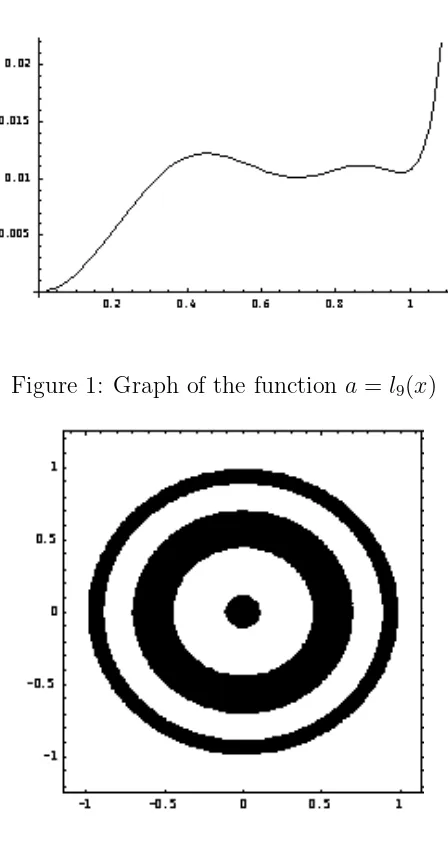
{Γ(a)} can be characterized also by the x-coordinates of their intersection point with the positivex-axis, that means by the limit cycle functionl, which coincides in the present case with the Andronov-Hopf function. In a given small neighborhood of the origin the number of limit cycles can change by the occurrence of multiple limit cycles. In our case, we restrict to the neighborhood x2 +y2 ≤ 1.2 and use the limit cycle function lto investigate the appearance of multiple limit cycles. By applying the numerical procedure described in the section before we compute l(x) forx= 0.01 +j0.025, j = 1, ..,44. Then we approximate the obtained set of points by some polynomial lN of orderN. For this purpose we apply the method of least squares. We choose N in such a way that number of extrema of the polynomiallN in the interval [0.01,1.085] does not change if we increase N. By this way, we have got the result
l9(x) = 0.154224x2+ 0.124769x3−1.63087x4
+ 3.22805x5−5.36163x6+ 8.75029x7−7.9267x8+ 2.6726x9.
By means of Sturm’s chains we can prove that the polynomiall9 has in the interval [0.01,1.085] exactly four extrema: the pointsA(0.4522,0.0121) andC(0.8726,0.0111) are minima, the points B(0.6952,0.0101) and D(0.9758,0.0105) are maxima. The graph of the function a=l9(x) is represented in Fig. 1. From these investigations we can conclude that system (5.1) has at least five limit cycles for 0.0105003≤a≤
Figure 1: Graph of the functiona =l9(x)
Figure 2: Ovals defined by Ψ(x, y) = 0
6
Acknowledgement
The second author acknowledgements the financial support by DAAD and the hos-pitality of the Weierstrass Institute for Applied Analysis and Stochastics in Berlin.
References
[1] A. A. Andronov, E. A. Leontovich, I. I. Gordon, A. G. Maier,
Qual-itative theory of second order dynamical systems, John Wiley and Sons, New York, 1973.
[2] L. A. Cherkas, The question on the analyticity of a manifold determining limit cycles, Differential Equations18(1982), 839-845.
[3] L. A. Cherkas, Dulac function for polynomial autonomous systems on a
plane, Differential Equations33 (1997), 692-701.
[4] L. A. Cherkas, J. C. Artes, J. Llibre,Quadratic systems with limit cycles of normal size, Bul. Acad. Stiinte Rep. Mold., Matematica. 41(2003), 31-46.
[5] L. A. Cherkas, A. A. Grin,Algebraic aspects of finding a Dulac function for polynomial autonomous systems on the plane, Differential Equations37(2001), 411-417.
[6] F. Dumortier, J. Llibre, J. C. Artes,Qualitative theory of planar differ-ential systems, Universitext. Springer, 2006.
[7] A. A. Grin, L. A. Cherkas,Dulac function for Li´enard systems(in Russian), Transactions Inst. Math. Belorus. Nat. Acad. Sci., Minsk,4 (2000), 29-38.
[8] A. A. Grin, L. A. Cherkas, Extrema of the Andronov-Hopf function of a
polynomial Li´enard system, Differential Equations41 (2005), 50-60.
[9] D. Hilbert, Mathematical Problems. Reprinted english translation: Bull.
Amer. Math. Soc. 37(2000), 407-436.
[10] L. Perko, Differential equations and dynamical systems, Texts Appl. Math. 7, Springer, 2001.
[11] L.P. Shilnikov, A.L. Shilnikov, D.V. Turaev, L.O. Chua, Methods of
qualitative theory in nonlinear dynamics. Part I, Part II, World Scientific Series on Nonlinear Science. Series A. 4,5. Singapore, 1998, 2001.
[12] S. Smale, Mathematical problems for the next century, Mathematical Intelli-gencer 20 (1998), 7-15.