Partition-Dependent Stochastic Measures
and
q-Deformed Cumulants
Michael Anshelevich
Received: June 26, 2001
Communicated by Joachim Cuntz
Abstract. On aq-deformed Fock space, we define multipleq-L´evy processes. Using the partition-dependent stochastic measures derived from such processes, we define partition-dependent cumulants for their joint distributions, and express these in terms of the cumulant func-tional using the number of restricted crossings of P. Biane. In the single variable case, this allows us to define aq-convolution for a large class of probability measures. We make some comments on the Itˆo table in this context, and investigate theq-Brownian motion and the
q-Poisson process in more detail.
2000 Mathematics Subject Classification: Primary 46L53; Secondary 05A18, 47D, 60E, 81S05
1. Introduction
In [RW97], Rota and Wallstrom introduced, in the context of usual probability theory, the notion of partition-dependent stochastic measures. These objects give precise meaning to the following heuristic expressions. Start with a L´evy processX(t). For a set partitionπ= (B1, B2, . . . , Bk), temporarily denote by
c(i) the number of the classBc(i)to whichibelongs. Then, heuristically, Stπ(t) =
Z
[0,t)k allsi’s distinct
dX(sc(1))dX(sc(2))· · ·dX(sc(n)).
In particular, denote by ∆nthe higher diagonal measures of the process defined by
∆n(t) =
Z
[0,t)
(dX(s))n.
The formulation of the algebraic (noncommutative, quantum) probability goes back to the beginnings of quantum mechanics and operator algebras. While a number of results have been obtained in a general context, in many cases the lack of tight hypotheses guaranteed that the conclusions of the theory would be somewhat loose. In the last twenty years of the twentieth century a particular noncommutative probability theory, the free probability theory [VDN92, Voi00], appeared, whose wealth of results approaches that of the clas-sical one. This theory is based on a new notion of independence, the so-called
free independence. In particular, one defines the (additive) free convolution, a new binary operation on probability measures: µ⊞ν is the distribution of the sum of freely independent operators with distributions µ, ν. Note that this is precisely the relation between independence and the usual convolution. Many limit theorems for independent random variables carry over to free prob-ability [BP99] by adapting the method of characteristic functions, using the
R-transform of Voiculescu in place of the Fourier transform. Applications of the theory range from von Neumann algebras to random matrix theory and asymptotic representations of the symmetric group.
In [Ans00, Ans01a] (see also [Ans01b]) we investigated the analogs of the mul-tiple stochastic measures of Rota and Wallstrom in the context of free proba-bility theory. In this analysis, the starting object X(t) is a stationary process withfreelyindependentbounded increments. One important fact observed was that in the classical case the expectation of Stπ(t) is the combinatorial cumu-lant of the distribution of X(t). This means that the expectation of Stπ(t) is equal toQkj=1r|Bj|, whereri is thei-th coefficient in the Taylor series expan-sion of the logarithm of the Fourier transform of the distribution ofX(t). See [Shi96, Nic95] or Section 6.1. The importance of cumulants lies in their relation to independence: since independence corresponds to a factorization property of the joint Fourier transforms, it can also be expressed as a certain additivity property of cumulants, the “mixed cumulants of independent quantities equal 0” condition. See Section 4.1.
the symmetric and anti-symmetric Fock spaces, respectively). For the interme-diate values ofq, it is known that the theory cannot be as good as the classical and the free ones, since one cannot define a notion ofq-independence satisfying all the desired properties [vLM96, Spe97b].
In this paper we try a different approach. As mentioned above, whenever we have a family of operators which corresponds to a family of measures that is in some sense infinitely divisible, we should be able to define the partition-dependent stochastic measures, and thendefinethe combinatorial cumulants as their expectations. One definition of cumulants appropriate for theq-deformed probability theory has already been given in [Nic95], based on an analog of the canonical form introduced by Voiculescu in the context of free probability. The advantage of the approach of that paper is that Nica’s cumulants are de-fined for any probability distribution all of whose moments are finite. However, the canonical form of that paper is not self-adjoint, and it is also not appro-priate for our approach since it does not provide us with a natural additive process. Instead, as a canonical form we choose theq-analog of the families of [HP84, AH84, Sch91, GSS92], which in the classical and the free case provide representations for all (classically, resp. freely) infinitely divisible distributions all of whose moments are finite. We provide an explicit formula for the result-ing combinatorial cumulants, involvresult-ing as expected a notion of the number of crossings of a partition. The appropriate one for our context happens to be the number of “restricted crossings” of [Bia97]; in particular the resulting cu-mulants are different from those of [Nic95]. Our approach makes sense only for distributions corresponding to q-infinitely divisible families (although strictly speaking, one can use our definition in general). However, our canonical form of an operator is self-adjoint, and this in turn leads to a notion ofq-convolution on a large class of probability measures. The fact that this convolution is not defined on all probability measures is actually to be expected, see Section 6.1. After finishing this article, we learned about a physics paper [NS94] which seems to have been overlooked by the authors of both [Bia97] and [SY00b]. The goals of that paper are different from ours, but in particular it defines and investigates the sameq-Poisson process as we do (Section 6.3) and, in that case, points out the relation between the moments of the process and the number of restricted crossings of corresponding partitions. It would be interesting to see if the results of that paper can be extended to our context, and how our results fit together with the “partial cumulants” approach.
this context, by calculating the quadratic co-variation of twoq-L´evy processes. In a long Section 6 we define theq-convolution, describe how our construction relates to the Bercovici-Pata bijection, and investigate theq-Brownian motion and theq-Poisson process in more detail. Finally, in the last section we make a few preliminary comments on the von Neumann algebras generated by the processes.
Acknowledgments: I would like to thank Prof. Bo˙zejko for encouraging me to look at theq-analogs of [Ans00], and Prof. Voiculescu for many talks I had to give in his seminar, during which I learned the background for this paper. I am also grateful to Prof. Speicher for a number of suggestions about Section 7, and to Daniel Markiewicz for numerous comments. This paper was written while I was participating in a special Operator Algebras year at MSRI, and is supported in part by an MSRI postdoctoral fellowship.
2. Preliminaries
2.1. Notation. Fix a parameterq∈(−1,1); we will usually omit the depen-dence onqin the notation. The analogs of the results of this paper forq=±1 are in most cases well-known; we will comment on them throughout the pa-per. Forna non-negative integer, denote by [n]q the corresponding q-integer, [0]q = 0, [n]q =Pni=0−1qi.
For a collection nyj(i)o of numbers and two multi-indices~v= (v(1), . . . , v(k)) and ~u= (u(1), . . . , u(k)), we will throughout the paper use the notation y(~~vu)
to denote Qkj=1yv(j)(u(j)).
Denote by [k . . . n] the ordered set of integers in the interval [k, n].
For a family of functions{Fj}, whereFjis a function ofjarguments,~va vector withkcomponents, and B⊂[1. . . k], denoteF(~v) =Fk(~v) and
F(B :~v) =F|B|(v(i(1)), v(i(2)), . . . , v(i(|B|))),
where B= (i(1), i(2), . . . , i(|B|)). In particular, we use this notation for joint moments and cumulants (see below).
2.2. Partitions. For an ordered setS, denote byP(S) the lattice of set par-titions of that set. Denote by P(n) the lattice of set partitions of the set [1. . . n], and byP2(n) the collection of its pair partitions, i.e. of partitions into 2-element classes. Denote by ≤ the lattice order, and by ˆ1n = ((1,2, . . . , n)) the largest and by ˆ0n= ((1)(2). . .(n)) the smallest partition in this order. Fix a partitionπ∈ P(n), with classes{B1, B2, . . . , Bl}. We writeB ∈πifB is a class ofπ. Call a class ofπa singletonif it consists of one element. For a classB, denote bya(B) its first element, and byb(B) its last element. Order the classes according to the order of their last elements, i.e. b(B1)< b(B2)< . . . < b(Bl). Call a class B ∈ πan interval if B = [a(B). . . b(B)]. Call πan
interval partition if all the classes ofπare intervals.
p(i) = max{j∈B, j < i}. For two classes B, C ∈ π, a restricted crossing is a quadruple (p(i) < p(j) < i < j) with i ∈ B, j ∈ C. The number of restricted crossings ofB, C is
rc (B, C) =|{i∈B, j∈C:p(i)< p(j)< i < j}| +|{i∈B, j∈C:p(j)< p(i)< j < i}|,
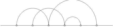
and the number of restricted crossings ofπis rc (π) =Pi<jrc (Bi, Bj). It has the following graphical representation. Draw the points [1. . . n] in a sequence on thex-axis, and to represent the partitionπconnect eachiwithp(i) (if it is well-defined) by a semicircle above thexaxis. Then the number of intersections of the resulting semicircles is precisely rc (π). See Figure 1 for an example. We say that a partition πis noncrossing if rc (π) = 0. Denote by NC(n)⊂ P(n) the collection of all noncrossing partitions, which in fact form a sub-lattice of P(n).
Figure 1. A partition of 6 elements with 2 restricted crossings. We need some auxiliary notation. For σ, π∈ P(n), we defineπ∧σ∈ P(n) to be the meet ofπandσin the lattice, i.e.
iπ∼∧σj ⇔ i∼π j andi∼σ j.
Forπ∈ P(n), we defineπop
∈ P(n) to be πtaken in the opposite order, i.e.
iπ∼opj ⇔ (n−i+ 1)∼π (n−j+ 1).
Forπ∈ P(n), σ∈ P(k), we defineπ+σ∈ P(n+k) by
iπ+σ∼ j ⇔((i, j≤n, i∼π j) or (i, j > n,(i−n)∼σ (j−n))).
We’ll denotemπ=π+π+. . .+π mtimes.
Finally, using the above notation, for a subset B ⊂ [1. . . n] and π ∈ P(n), (B:π) is the restriction ofπtoB.
2.3. The q-Fock space. Let H be a (complex) Hilbert space. Let Falg(H) be its algebraic full Fock space,Falg(H) =L∞n=0H⊗n, where H⊗0=CΩ and Ω is the vacuum vector. For eachn≥0, define the operatorPn onH⊗n by
P0(Ω) = Ω,
Pn(η1⊗η2⊗. . .⊗ηn) =
X
α∈Sym(n)
where Sym(n) is the group of permutations of n elements, and i(α) is the number of inversions of the permutation α. For q = 0, each Pn = Id. For
q= 1, Pn =n! ×the projection onto the subspace of symmetric tensors. For
q=−1,Pn=n!×the projection onto the subspace of anti-symmetric tensors. Define theq-deformed inner product onFalg(H) by the rule that forζ∈H⊗k,
η∈H⊗n,
hζ, ηiq =δnkhζ, Pnηi,
where the inner product on the right-hand-side is the usual inner product in-duced on H⊗n from H. All inner products are linear in the second variable. It is a result of [BS91] that the inner product h·,·iq is positive definite for
q∈(−1,1), while for q=−1,1 it is positive semi-definite. LetFq(H) be the completion of Falg(H) with respect to the norm corresponding to h·,·iq. For
q = −1,1 one first needs to quotient out by the vectors of norm 0 and then complete; the result is the anti-symmetric, respectively, symmetric Fock space, with the inner product multiplied byn! on then-particle space.
ForξinH, define the (left) creation and annihilation operators onFalg(H) by, respectively,
a∗(ξ)Ω =ξ,
a∗(ξ)η1⊗η2⊗. . .⊗ηn=ξ⊗η1⊗η2⊗. . .⊗ηn, and
a(ξ)Ω = 0, a(ξ)η =hξ, ηiΩ,
a(ξ)η1⊗η2⊗. . .⊗ηn = n
X
i=1
qi−1hξ, ηiiη1⊗. . .⊗ηˆi⊗. . .⊗ηn,
where as usual ˆηimeans omit thei-th term. Forq∈(−1,1), both operators can be extended to bounded operators onFq(H), on which they are adjoints of each other [BS91]. They satisfy the commutation relationsa(ξ)a∗(η)
−qa∗(η)a(ξ) =
hξ, ηiId.Forq=±1, we first need to compress the operators by the projection onto the symmetric / anti-symmetric Fock space, respectively, and the resulting operators differ from the usual ones by√n, but satisfy the usual commutation relations (thanks to a different inner product). Forq= 1 the resulting operators are unbounded, but still adjoints of each other [RS75].
Denote byϕthe vacuum vector stateϕ[X] =hΩ, XΩiq.
Another choice for the number operator is the operator that has H⊗n as an eigenspace with eigenvalue [n]q. For a general (bounded) operatorT, the cor-responding construction is
p(T)Ω = 0,
p(T)η1⊗η2⊗. . .⊗ηn= n
X
i=1
qi−1η
1⊗. . .⊗(T ηi)⊗. . .⊗ηn.
Similar operators were used in [´Sni00], where stochastic calculus with respect to the corresponding processes was developed. They do have nice commutation properties, but are in general not symmetric.
Finally, another natural choice for the number operator isPia∗(ei)a(ei), where
{ei}is an orthonormal basis forH; the resulting operator is then independent of the choice of the basis. For a general bounded operator T, the correspond-ing construction is Pia∗(T ei)a(ei). It is easy to see that this sum converges
strongly, to the following operator.
Definition 2.1. LetT be an operator on H with dense domainD. The cor-responding gauge operator p(T) is an operator on Fq(H) with dense domain Falg(D) defined by
p(T)Ω = 0,
p(T)η1⊗η2⊗. . .⊗ηn= n
X
i=1
qi−1(T ηi)
⊗η1⊗. . .⊗ηˆi⊗. . .⊗ηn,
forη1, η2, . . . , ηn∈ D.
Proposition 2.2. If T is essentially self-adjoint on a dense domain D and
T(D)⊂ D, then p(T)is essentially self-adjoint on a dense domainFalg(D). Proof. We first show thatp(T) is symmetric onFalg(D). Fixn, and denote by
βjthe cycle in Sym(n) given byβj= (12. . . j). For a permutationα∈Sym(n), writeα(η1⊗. . .⊗ηn) =ηα(1)⊗. . .⊗ηα(n). Forη1, . . . , ηn, ξ1, . . . , ξn ∈ D,
hp(T)η1⊗. . .⊗ηn, ξ1⊗. . .⊗ξniq
=
n
X
j=1
qj−1
β−j1(η1⊗. . .⊗(T ηj)⊗. . .⊗ηn), ξ1⊗. . .⊗ξn®q
=
n
X
j=1
X
α∈Sym(n)
qj−1qi(α)
βj−1(η1⊗. . .⊗(T ηj)⊗. . .⊗ηn), α(ξ1⊗. . .⊗ξn)®
=
n
X
j=1
n
X
k=1
X
α∈Sym(n)
α(1)=k
qj−1qi(α)
βj−1(η1⊗. . .⊗ηn), α(ξ1⊗. . .⊗(T∗ξk)⊗. . .⊗ξn)®
=
n
X
j=1
n
X
k=1
X
α∈Sym(n)
α(1)=k
qj−1qi(α)
Using the combinatorial lemma immediately following this proof, this expres-sion is equal to
=
n
X
k=1
X
γ∈Sym(n)
qk−1qi(γ)
η1⊗. . .⊗ηn, γ(β−k1(ξ1⊗. . .⊗(T∗ξk)⊗. . .⊗ξn))®
=hη1⊗. . .⊗ηn, p(T∗)ξ1⊗. . .⊗ξniq.
Now we show that the operatorp(T) is essentially self-adjoint onFalg(D). For
q = 1, the proof is contained in [RS75, X.6, Example 3]. For q ∈(−1,1) we proceed similarly. LetDn=D⊗n. LetE·be the spectral measure of the closure
¯
T ofT, andC∈R+. Let{ηi}n
i=1⊂(E[−C.C]H)∩ D; thenkT ηik ≤Ckηik. Let
~η=η1⊗η2⊗. . .⊗ηn. Then
°
°p(T)k~η°°2q =p(T)k~η, Pnp(T)k~η
®
≤ kPnk(nkCkk~ηk)2. It was shown in [BS91] thatkPnk ≤[n]|q|!≤n!. We conclude that
°
°p(T)k~η°° q ≤ √
n!nkCk
k~ηk and so
lim sup k→∞
1
k °
°p(T)k~η°°1/k
q = 0.
Therefore ~η is an analytic vector for p(T). The linear span of such vectors is invariant under p(T) and is a dense subset of Dn. Therefore by Nelson’s analytic vector theorem,p(T) is essentially self-adjoint onDn.
The rest of the argument proceeds as in [RS72, VIII.10, Example 2]. An operatorAis essentially self-adjoint iff the range ofA±iis dense. Sincep(T) restricted to H⊗n is essentially self-adjoint, this property holds for each such restriction, and then for the operator p(T) itself, which therefore has to be essentially self-adjoint.
Lemma 2.3. For a fixed k, every permutationγ ∈Sym(n)appears in the col-lection
{βjαβk : 1≤j≤n, α(1) =k}
exactly once. Moreover, for suchα,i(βjαβk) =i(α) +j−k.
Proof. It suffices to show the first property for the collection {βjα}. This collection contains at most n! distinct elements. On the other hand, for γ ∈
Sym(n), letj = γ−1(k), and α =β−1
j γ; then j, α satisfy the conditions and
βjα=γ.
For the second property, first take γ ∈Sym(n) such that γ(1) = 1 and show thati(βjγ) =i(γ) + (j−1). Indeed,βj only reverses the order of (j−1) pairs (a, j) witha < j. βj sends such a pair to ((a+ 1),1), and since γ(1) = 1, γ preserves the order of such a pair.
We conclude that i(βjαβk) = i(αβk) + (j−1). Now we show that i(αβk) =
i(α)−(k−1). Indeed, βk only reverses the order of (k−1) pairs (a, k) for
These gauge operators themselves do not satisfy nice commutation relations. Nevertheless, we can still calculate their combinatorial cumulants. Another advantage of this definition is that it naturally generalizes to the “Yang-Baxter” commutation relations of [BS94]. However, in this more general con-text partition-dependent cumulants are not expressed in terms of the cumulant functional, so we do not pursue this direction in more detail.
For q = 0, p(T) are precisely the gauge operators on the full Fock space as defined in [GSS92]. Forq= 1, again we first need to compressp(T) by the pro-jection onto the symmetric Fock space, and the result is the usual differential second quantization. Forq=−1, we first need to compressp(T) by the projec-tion onto the anti-symmetric Fock space, and the result is the anti-symmetric differential second quantization.
2.5. The processes. LetV be a Hilbert space, and letHbe the Hilbert space
L2(R
+, dx)⊗V. Letξ∈V, and letT be an essentially self-adjoint operator on a dense domain D ⊂V so thatDis equal to the linear span of {Tnξ
}∞n=0 and moreoverξis an analytic vector forT. Given a half-open intervalI⊂R+, define
aI(ξ) =a(1I⊗ξ),a∗I(ξ) =a∗(1I⊗ξ),pI(T) =p(1I⊗T). Here1Iis the indicator function of the setI, considered both as a vector inL2(R+) and a multiplication operator on it. Forλ∈R, denote pI(ξ, T, λ) =aI(ξ) +a∗I(ξ) +pI(T) +|I|λ.
Denote byat, a∗t, ptthe appropriate objects corresponding to the interval [0, t). We will call a process of the form I7→pI(ξ, T, λ) aq-L´evy process. Forq= 1 this is indeed a L´evy process.
Now fix a k-tuple {Tj}kj=1 of essentially self-adjoint operators on a common dense domain D ⊂ V, Tj(D) ⊂ D, a k-tuple {ξj}kj=1 ⊂ D of vectors, and {λj}kj=1⊂R. We will make an extra assumption that
∀i, j∈[1. . . k], l∈N, ~u∈[1. . . k]l,
T~uξi=Tu(1)Tu(2). . . Tu(l)ξi is an analytic vector forTj, andD= span¡©T~uξi:i∈[1. . . k], l∈N, ~u∈[1. . . k]l
ª¢ .
(1)
Denote by X the k-tuple of processes (X(1), . . . , X(k)), where X(j)(I) =
pI(ξj, Tj, λj). In particular X(t) = X([0, t)). We call such a k-tuple a
mul-tipleq-L´evy process.
Remark 2.4. The assumption (1) is not essential for most of the paper. Most of the analysis could be done purely algebraically: see Remark 5.1. We will make this assumption to guarantee that we have a correspondence between self-adjoint processes and semigroups of measures, rather than between symmetric processes and semigroups of moment sequences.
3. Cumulants
Denote by Chxi = Chx1, x2, . . . , xki the algebra of polynomials in k formal
noncommuting indeterminates with complex coefficients. Note that in a more abstract language, this is just the tensor algebra of the complex vector space
V0 with a distinguished basis{xi}ki=1. While we take V0 to be k-dimensional, the same arguments will work for an arbitrary V0, as long as we use a more functorial definition of a process, namely forf =Paixi∈V0, we would define
T(f) =PaiTi, ξ(f) =Paiξi, λ(f) =Paiλi. See [Sch91] for a more detailed description of this approach.
Define a functional M on Chxi by the following action on monomials:
M(1, t;X) = 1, for a multi-index~u,
M(x~u, t;X) =ϕ
h
X(~u)(t)i,
and extend linearly. We will call M(·, t;X) the moment functional of the processXat timet.
If we equipChxiwith a conjugation∗extending the conjugation onCso that
eachx∗
i =xi, it is clear thatM is a positive functional, i.e.M(f f∗, t;X)≥0 for allf ∈Chxi.
For a partitionπ∈ P(n) and a monomialx~uof degreen, denoteMπ(x~u, t;X) =
Q
B∈πM(x(B:~u), t;X). These are the combinatorial moments ofXat timet. For a one-dimensional process, the functional M(·, t;X) can be extended to a probability measure µt such thatµt(xn) =M(xn, t;X). Specifically, µt(S) =
ϕ[ES], where E·is the spectral measure ofX(t).
3.2. Multiple stochastic measures and cumulants. For a set S and a partitionπ∈ P(n), denote
Sπn=
n
~v∈Sn:v(i) =v(j)⇔i∼π jo
and
Sn≤π=
n
~v∈Sn:v(i) =v(j)⇒i∼π jo.
Fixt. ForN ∈Nand a subdivision of [0, t) intoNdisjoint ordered half-open
in-tervalsI ={I1, I2, . . . , IN}, letδ(I) = max1≤i≤N|Ii|. DenoteXi, ai, a∗i, pi the appropriate objects for the intervalIi. Fix a monomialx~u∈Chx1, x2, . . . , xki of degreen.
Definition 3.1. The stochastic measure corresponding to the partition π, monomialx~u, and subdivisionI is
Stπ(x~u, t;X,I) =
X
~ v∈[1...N]n
π
X(~~vu).
The stochastic measure corresponding to the partitionπand the monomialx~u is
Stπ(x~u, t;X) = lim
if the limit, along the net of subdivisions of the interval [0, t), exists. In partic-ular, denote by ∆n(x~u, t;X,I) = Stˆ1(x~u, t;X,I) and
∆n(x~u, t;X) = Stˆ1(x~u, t;X) then-dimensionaldiagonal measure.
Definition 3.2. The combinatorial cumulant corresponding to the partition
πand the monomialx~u is
Rπ(x~u, t;X) = lim
δ(I)→0ϕ[Stπ(x~u, t;X,I)] if the limit exists. In particular, denote by
R(x~u, t;X) =Rˆ1(x~u, t;X) = lim
δ(I)→0ϕ[∆n(x~u, t;X,I)]
the n-th joint cumulant of X at time t. Note that the functional R(·, t;X) can be linearly extended to all of Chxi. We call this functional thecumulant functional of the process X at time t. For t = 1 we call the corresponding functional the cumulant functional of the processX.
We will omit the dependence onXin the notation if it is clear from the context. Clearly if Stπ(x~u, t) is well-defined, its expectation is equal toRπ(x~u, t). By definition ofSn
π, for anyI
X(~u)(t) = X π∈P(n)
Stπ(x~u, t;X,I). (2)
If Stπ(x~u, t) are well-defined, then
X(~u)(t) = X π∈P(n)
Stπ(x~u, t;X),
and so
M(x~u, t;X) =
X
π∈P(n)
Rπ(x~u, t;X); (3)
in fact for this last property to hold it suffices that the combinatorial cumulants exist.
The following general algebraic notion of independence is due to K¨ummerer.
Lemma 3.3. A multipleq-L´evy process X(t) has pyramidally independent in-crements. That is, for a family of intervals n{Ii}i=1n1+n3,{Jj}nj=12
o
in R+ such that for all i, j,Ii∩Jj =∅,
ϕ
Ãn1
Y
i=1
X(u(i))(Ii)
!
n2 Y
j=1
X(v(j))(Jj)
Ãn1+n3 Y
i=n1+1
X(u(i))(Ii)
!
=ϕ "n1+n3
Y
i=1
X(u(i))(Ii)
#
ϕ
n2 Y
j=1
X(v(j))(Jj)
Proposition 3.5. For a noncrossing partitionσ,
Mσ(x~u, t;X) =
X
π∈P(n) π≤σ
Rπ(x~u, t;X)
if the combinatorial cumulants are well-defined.
Proof. A noncrossing partition is determined by the property that it contains a class that is an interval and the restriction of the partition to the complement of that class is still noncrossing. Using this fact and Lemma 3.3, we can conclude that forπ∈ P(n), π≤σand~v∈[1. . . N]n
π,
ϕhX~(~vu)i= Y B∈σ
ϕhX(B:~(B:~u)v)i.
Therefore
ϕ[Stπ(x~u, t;X,I)] =
Y
B∈σ
ϕ£St(B:π)(x(B:~u), t;X,I)
¤ .
Thus if the combinatorial cumulants are well-defined,
Rπ(x~u, t;X) =
Y
B∈σ
R(B:π)(x(B:~u), t;X),
and so
X
π∈P(n) π≤σ
Y
B∈σ
R(B:π)(x(B:~u), t;X) =
X
π∈P(n) π≤σ
Rπ(x~u, t;X).
Ifσ= (B1, B2, . . . , Bl), the left-hand-side of this equation is equal to l
Y
i=1
X
πi∈P(Bi)
Rπi(x(Bi:~u), t;X).
Combining this equation with equation (3), we obtain
Mσ(x~u, t;X) =
X
π∈P(n) π≤σ
Rπ(x~u, t;X).
We emphasize that while σ is noncrossing, π need not be. Note that on the operator level we have for anyσ∈ P(n),
X
π∈P(n) π≤σ
Stπ(x~u, t;X,I) =
X
~ v∈[1...N]n
≤σ
X(~~vu).
Proposition 3.6. For the monomialx~u of degree n, the cumulant functional
of the multiple q-L´evy process Xis given by
R(x~u, t) =
(
tλu(1) ifn= 1,
tDξu(1),Qnj=2−1Tu(j)ξu(n)
E
Proof. By definition,
Here the sum is taken over all decompositions of [1. . . n] into four disjoint subsetsS1, S2, S3, S4, and for each choice of these subsets
We show that the limit of each of the remaining terms is 0. Indeed,
whereCis a constant independent of the subdivisionI. Therefore such a term converges to 0 asδ(I)→0.
Construction 3.7 (An un-crossing map). Fix a partition π with l classes
B1, . . . , Bl. In preparation for the next theorem, we need the following com-binatorial construction. Define the map F : P(n) → P(n) as follows. If π
is an interval partition, F(π) =π. Otherwise, let i be the largest index of a non-interval classBiofπ. Letj2= max{s∈Bi : (s−1)6∈Bi}andj1=p(j2). Letαbe the power of a cycle permutation
((j1+ 1)(j1+ 2). . . b(Bi))b(Bi)−j2+1.
Then F(π) = α◦π, by which we meani ∼π j ⇔ α(i) F(π)∼ α(j). Also define
cb(π) =|{s:j1< b(Bs)< b(Bi)}| − |{s:j1< a(Bs)< b(Bi)}|. Then rc (π) = rc (F(π))+cb(π). Indeed, forB, C ∈π, B, C=6 Bi, rc (B, C) = rc (α(B), α(C)). The number of restricted crossings of Bi, Bj with bi ∈ Bi, bj ∈ Bj and
p(bi) < p(bj) < bi < bj ≤ j1 or p(bj) < p(bi) < bj < bi ≤ j1 is equal to the corresponding number forα(Bi), α(Bj), while there are no restricted cross-ings forbi> j2forBi andbi> j1 forα(Bi). Finally, there arecb(π) restricted crossings of the formp(j)< j1< j < j2in π. See Figure 2 for an example.
Figure 2. Iteration ofF on a partition of 6 elements. ClearlyFn(π) is an interval partition. ThereforePn
s=0cb(Fsπ) = rc (π).
Theorem 3.8. The combinatorial cumulants can be expressed in terms of the cumulant functional: for π∈ P(n)andx~u a monomial of degreen,
Rπ(x~u, t) =qrc(π) l
Y
i=1
R(x(Bi:~u), t).
Proof. The same argument as in the previous proposition shows that
Rπ(x~u, t) = lim δ(I)→0ϕ
X
~ v∈[1...N]n
π
yv(1)(1) yv(2)(2) . . . yv(n)(n)
,
with
yi(j)=
|Ii|λu(j) if (j) is a singleton inπ,
ai(ξu(j)) ifj is the first element of its class inπ, a∗
i(ξu(j)) ifj is the last element of its class inπ,
pi(Tu(j)) otherwise.
Fix~v. LetBbe the class ofπcontainingn. IfB is an interval, then by Lemma
Remark 3.9 (Comments on Proposition 3.5). Forq= 0,Rπ(x~u, t;X) = 0 un-lessπis noncrossing. Then forσ∈NC(n),
Mσ(x~u, t;X) =
X
π∈NC(n) π≤σ
Rπ(x~u, t;X).
Therefore forπ∈NC(n),
Rπ(x~u, t;X) =
X
σ∈NC(n) σ≤π
M¨obNC(σ, π)Mσ(x~u, t;X),
where M¨obNC is the M¨obius function on the lattice of noncrossing partitions. Forq= 1, ifσ∈ P(n),σ= (B1, B2, . . . , Bl), then
Mσ(x~u, t;X) = l
Y
i=1
M(x(Bi:~u), t;X)
= l
Y
i=1
X
πi∈P(Bi)
Rπi(x(Bi:~u), t;X)
=X
π≤σ
Rπ(x~u, t;X).
Therefore forπ∈ P(n),
Rπ(x~u, t;X) =
X
σ∈P(n) σ≤π
M¨obP(σ, π)Mσ(x~u, t;X),
where M¨obP is the M¨obius function on the lattice of all partitions. Note that X(I) commute withX(J) forI∩J =∅on the symmetric Fock space.
Thus forq= 0,1, the cumulant functional at time 1 can be expressed through the moment functional at time 1. We will show how to do this for arbitraryq
in the next section.
4. Characterization of generators
Denote byR(f;X) =R(f,1;X) the cumulant functional.
Lemma 4.1. The family of the moment functionals of a multipleq-L´evy process is determined by its cumulant functional. The functional R(·;X) on Chxi is the generator of the family of functionals M(·, t;X), that is,
d dt ¯ ¯ ¯
Proof. It suffices to prove these statements for a monomialx~uof degreen. By equation (3), Theorem 3.8 and Proposition 3.6,
M(x~u, t;X) =
which implies the first statement. By differentiating this equality, we obtain
d
Definition 4.2. A functionalψonChxiisconditionally positiveif its restric-tion to the subspace of polynomials with zero constant term is positive semi-definite.
We say that the functionalψisanalytic if for anyiand any multi-index~u, lim sup
The following proposition is an analog of the Schoenberg correspondence for our context. Note that the formulation of the result does not involve q: the dependence onqis hidden in Theorem 3.8.
Proposition 4.3. A functionalψis analytic and conditionally positive if and only if it is the generator of the family of the moment functionals for some multipleq-L´evy process.
Proof. The proof is practically identical to that of [GSS92], or indeed of [Sch91]. We provide an outline for the reader’s convenience.
Supposeψ is the generator of the family of moment functionalsM(·, t;X) for a multiple q-L´evy processX(t) =pt(ξ,T, λ). From the fact that each of the moment functionals is positive and equals 1 on the constant 1 it follows by differentiating that the cumulant functional is conditionally positive. Since
Now suppose ψ is conditionally positive and analytic. Then it gives rise to a multiple q-L´evy process, as follows. Denote by δ0(f) the constant term of
f ∈Chxi. ψinduces a positive semi-definite inner product on the space Chxi
byhf, giψ =ψ[(f−δ0(f))∗(g
−δ0(g))]. Let Nψ be the subspace of vectors of length 0 with respect to this inner product. LetV be the Hilbert space obtained by completing the quotient (Chxi)/Nψwith respect to this inner product, with
the induced inner product. Denote byρthe canonical mapping Chxi →V, let Dbe its image, and forf, g∈Chxidefine the operator Γ(f) :D → Dby
Γ(f)ρ(g) =ρ(f g)−ρ(f)δ0(g).
The operator Γ is well defined since, by the Cauchy-Schwartz inequality, kΓ(f)ρ(g)kψ=ψ[(g−δ0(g))∗f∗f(g−δ0(g))]≤ kρ(g)kψkf∗f(g−δ0(g))kψ.
Clearly Dis dense inV, invariant under Γ(f), and Γ(f) is symmetric on it if
f is symmetric.
Put, for i ∈ [1. . . k], λi = ψ[xi], ξi =ρ(xi), Ti = Γ(xi). Each Ti takes D to itself. By construction, Γ(xi)ρ(x~u) =ρ(xix~u), and so
lim sup n→∞
1
nkT
n
i ρ(x~u)k1/nψ = lim sup n→∞
1
nkx
n ix~uk1/nψ
= lim sup n→∞
1
nψ[(x~u)
∗x2n
i x~u]1/2n<∞
since the functionalψis analytic. Therefore each of the vectorsρ(x~u) is analytic forTi, and the linear span of these vectors isD. In particular,Ti is essentially self-adjoint onD.
Define the multiple q-L´evy processXbyX(i)(t) =pt(ξ
i, Ti, λi). Then
R(x~u;X) =ψ[x~u]. Indeed, forn= 1
R(xi;X) =λi=ψ[xi]. Forn≥2,
R(x~u;X) =
*
ξu(1), n−1
Y
j=2
T(u(j))ξu(n)
+
=
*
ρ(xu(1)),
n−1
Y
j=2
Γ(xu(j))ρ(xu(n))
+
ψ
=
*
ρ(xu(1)), ρ( n
Y
j=2
xu(j))
+
ψ =ψ[
n
Y
j=1
xu(j)]
=ψ[x~u].
4.1. Product states. For arbitrary q, the relation in the proof of Lemma 4.1 can be inverted.
Definition 4.4. Let Φ be any functional onChxi. Define the functional Ψ = logq(Φ) on monomials recursively by
Ψ(x~u) = Φ(x~u)−
X
π∈P(n) π6=ˆ1
qrc(π) Y
B∈π
Ψ(x(B:~u))
and extend linearly.
The definition has the form Ψ(x~u) =
X
σ∈P(n)
c(σ) Y B∈σ
Φ(x(B:~u))
for some coefficient family {c(σ) :σ∈ P(k)}. For q= 1, Φ is the convolution exponential of Ψ [Sch91]. Lemma 4.1 and the discussion in Section 6 justify the notations Ψ = logq(Φ), Φ = expq(Ψ). Note that this operation on functionals appears to bear no relation to theq-exponential power series.
It is clear that for any q-L´evy process, R(·, t;X) = logqM(·, t;X) and, more-over, that M(·, t;X) = expq(tR(·;X)).
Definition 4.5. Let Φ1 be a functional on Chx1, x2, . . . , xk
1i, Φ2 a
func-tional on Chx1, x2, . . . , xk
2i. Define their product functional Φ1 ×q Φ2 on
Chx1, x2, . . . , xk
1+k2iby the “mixed cumulants are 0” rule:
logq(Φ1×qΦ2)(x~u) =
logq(Φ1)(x~u) if∀i, u(i)≤k1, logq(Φ2)(x~u) if∀i, u(i)> k1,
0 otherwise.
Note that it is more natural to think of this construction as taking the product of two one-parameter families of functionals,
expq(tlogq(Φ1))×qexpq(tlogq(Φ2)) = expq(tlogq(Φ1×qΦ2)). Denote
IDc(q, k) ={Φ : Φ =M(·,1;X) for somek-dimensionalq-L´evy processX}
=©Φ : logq(Φ) is conditionally positive and analytic
ª .
The notation stands for “combinatorially infinitely divisible”.
Lemma 4.6. ForΦ1∈ IDc(q, k1),Φ2∈ IDc(q, k2), their product functional is a state, that is, a positive functional that equals1 on the identity element. Proof. It suffices to show that Φ1×q Φ2 ∈ IDc(q, k1+k2). Let X1,X2 be the q-L´evy processes whose distributions at time 1 are Φ1,Φ2, respectively. Let X(i,1)(t) =pt(ξ
i,1, Ti,1, λi,1), X(i,2)(t) =pt(ξi,2, Ti,2, λi,2). Hereξi,1 ∈V1,
Ti,1 is an operator on V1 with domain D1, ξi,2 ∈ V2, Ti,2 is an operator on
V2 with domain D2. Let V = V1⊕V2. Identify ξi,1 with ξi,1⊕0, ξi,2 with 0⊕ξi,2, Ti,1 with
¡Ti,10
0 0
¢
and Ti,2 with
¡0 0 0Ti,2
¢
identification does not change the cumulants or the moments of the processes
X1,X2, and that condition (1) holds for the (k1+k2)-dimensional processX= (X(1,1), . . . , X(k1,1), X(1,2), . . . , X(k2,2)). Then Φ1×
qΦ2is equal toM(·,1;X).
For q = 1, the product state is the usual (tensor) product state, while for
q= 0 it is the (reduced) free product state. Already forq=−1, the situation is unclear. The parity of rc (π) can differ from the parity of the number of left-reduced crossings of [Nic95] even for partitions all of whose classes have even order. Therefore even for q =−1, our cumulants are different from the
q-cumulants of that paper. In particular, the results of [MN97] about graded independence do not apply. Note also that our product state construction is defined only on the polynomial algebrasChxi, not on general algebras. So we do not obtain a universal product in the sense of [Spe97b].
A state Φ is tracial if for alla, b, Φ(ab) = Φ(ba). Forq= 0,1, the product state of two tracial states is tracial [VDN92]. This property remains true for the q -Brownian motion (see below). However, the number of the restricted crossings of a partition is not invariant under cyclic permutations of the underlying set. For example, rc (((1,3,5)(2,4))) = 2 while rc (((1,3)(2,4,5))) = 1. So for general q, the product state of two tracial states need not be tracial.
5. The Itˆo table
In general we do not know how to calculate the partition-dependent stochastic measures Stπ(X); indeed we don’t expect a nice answer for a general process. In particular we don’t expect that a functional Itˆo formula exists for q-L´evy processes. However, one ingredient of it is present, namely, we can calculate all the higher diagonal measures. These are higher variations of the processes, and appear in the functional Itˆo formula for the free L´evy processes [Ans01b].
Remark 5.1 (Algebraic approach). Unless we are considering higher diagonal measures of a single one-dimensional process, for this section we also need a more general setup than the one we had before. First, we need to consider multiple processes whose components are of the form X(t) = pt(ξ, η, T, λ) =
at(ξ) +a∗
t(η) +pt(T) +tλ. Second, we no longer can requireT to be symmetric and λ to be real. The solution in [Sch91] is to require that T be a linear operator with domainD, not necessarily dense, so that the restriction ofT∗to
Dis a well-defined linear operator.
We describe briefly how to modify this paper for the algebraic context. The gauge operators are defined in the same way, and the multiple q-L´evy process are modified as in the previous paragraph, except that we drop the assumption (1). The moments and cumulants can be modified to include∗-quantities, i.e. use words in bothXandX∗ in the definitions, and consider them as function-als on Chx1, x2, . . . , xk, x∗
modify the formula for the cumulant functional in terms ofξ, η, T, λ. In the al-gebraic context, generators of the families of moment functionals for symmetric processes are precisely all the conditionally positive functionals.
For the Itˆo table, we first need a technical lemma.
Lemma 5.2. Forf, g∈L2(R+),
Proof. We repeatedly use the Cauchy-Schwartz inequality for sequences and functions:
common refinement of I,J′. Then
2 converges to 0 along the net of subdivisionsI asδ(I)→0.
More precisely, the quadratic co-variation of these processes is
∆2(x1x2, t; (X(1), X(2))) = [X(1), X(2)](t) =pt(T2∗ξ1, T1η2, T1T2,hξ1, η2i).
Here the convergence in the definition of∆ is the pointwise convergence on the dense set Falg(L2(R+)⊗ D).
wherey((1),i), y((2),j)are labels for rows, respectively, columns of the Itˆo table, andy(i,j) is the corresponding entry of the table. All of these are obtained by applying Lemma 5.2, possibly with one or both of f, g equal to 1[0,t). More precisely, we use equation (6a) for the productda(ξ1)da(ξ2), equation (6b) for the products da∗(η1)da(ξ2), dp(T1)da(ξ2), da(ξ1)dp(T2) and equation (6c) for
the productsda∗(η1)da∗(η2), dp(T1)da∗(η2), da∗(η1)dp(T2), dp(T1)dp(T2).
L2(R+), ζ is bounded, so it suffices to show that
lim known forq= 1 [HP84] (with a somewhat different set of convergence),q=−1 [AH84] and q= 0 [Spe91]; for the q-Brownian motion (T = 0) it was known for allq[´Sni00]. In all of these cases it is only a facet of a well-defined theory of stochastic integration.
Corollary 5.5. For a one-dimensional self-adjoint processX(t) =pt(ξ, T, λ)
andk≥2,
6. Single-variable analysis
Denote byMc (for “combinatorial”) the space of finite positive Borel measures onRall of whose moments are finite, and byM1c ⊂ Mcthe subset of probability
measures. Forµ∈ Mc considered as a functional onC[x], denote its moments
µ(xn) bymn(µ). Forµ ∈ M1
candn≥1, theq-cumulantsrn(µ) = (logqµ)(xn) are determined by
rn(µ) =mn(µ)− X π∈P(n)
π6=ˆ1
qrc(π)Y
B∈π
r|B|(µ).
(7)
The expressions for the first few cumulants in terms of the moments andqare
r1=m1,
r2=m2−m21,
r3=m3−3m2m1+ 2m31,
r4=m4−4m3m1−(2 +q)m22+ (10 + 2q)m2m12−(5 +q)m41,
r5=m5−5m4m1−(5 + 4q+q2)m3m2+ (15 + 4q+q2)m3m21
+ (15 + 12q+ 3q2)m22m1−(35 + 20q+ 5q2)m2m31+ (14 + 8q+ 2q2)m51. While these cumulants are well-defined for arbitraryµ ∈ M1
c, our results ap-ply only to a special class of them. For a sequence r = (r0 = 0, r1, r2, . . .) in R, let ψr be the functional onC[x] defined byψr(Pn
i=0aixi) =Pni=0airi. The functionalψris analytic iff lim supn→∞n1r
1/2n
2(n+2)<∞. It is conditionally positive iff the functional ψ(r2,r3,...) is positive semi-definite. These
condi-tions imply [Shi96] that for n ≥ 0, rn+2 = mn(τ) for someτ ∈ Mc that is uniquely determined by its moments. Denote byMu (for “unique”) the sub-space of finite positive Borel measures in Mc that are of this form, i.e. for which lim supn→∞n1m2n(τ)
1/2n <
∞. Equivalently,τ∈ Mu if its exponential moment-generating functionRRexp(θx)dτ(x) is defined forθin a neighborhood of 0.
Definition 6.1. Letτ ∈ Mu, andλ∈R. Define LH−1
q (λ, τ) to be the prob-ability measure in M1
c determined by the cumulant sequence r1 = λ, rn =
mn−2(τ) for n ≥2. Equivalently, LH−q1(λ, τ) is the distribution at time 1 of theq-L´evy processpt(ξ, T, λ) such that the operatorT has distributionτ with respect to the vector functionalhξ,·ξi. Note that LHq−1(λ, τ) is in fact inM1u. Denote by IDc(q) the image of the map LH−q1; clearly IDc(q) = IDc(q,1). Call a measure inIDc(q)q-infinitely divisible.
It is clear that LH−q1 is injective. We define LHq : IDc(q) →R× Mu to be the inverse of LH−q1. This is an analog of the L´evy-Hinchin representation, or more precisely of the canonical representation; see Section 6.1.
1, andT corresponds to the operator of multiplication by the variable x. The Hilbert space H is then equal toL2(R
+×R, dx⊗τ).
Definition 6.2. For µ, ν ∈ IDc(q), define their q-convolution µ∗qν by the rule that LHq(µ∗qν) = LHq(µ) + LHq(ν).
Lemma 6.3. (IDc(q),∗q) is an Abelian semigroup. In particular, the q
-convolution of two positive measures is positive.
Proof. The sum of two measures inMu is inMu.
Lemma 6.4 (Relation to product states). Forµ1, µ2∈ IDc(q), (µ1∗qµ2)(xn) = (µ1×qµ2)((x1+x2)n).
Proof. Using the representation from the proof of Lemma 4.6, letξ=ξ1⊕ξ2∈
V,T =¡T1 0
0 T2 ¢
an operator onV with domainD1⊕D2,λ=λ1+λ2. LetV′be the closure of the span³©Tjξª∞j=0´. ThenT³span³©Tjξª∞j=0´´⊂V′. Define
T′ to be the restrictionT ↾V′. ThenX(t) =pt(ξ, T′, λ) is a q-L´evy process.
Its distribution is equal to µ1∗qµ2. Indeed, if we denote this distribution by
µ, then
r1(µ) =λ=λ1+λ2=r1(µ1) +r1(µ2), and forn≥2,
rn(µ) =ξ,(T′)n−2ξ®=ξ1, T1n−2ξ1
®
+ξ2, T2n−2ξ2
®
=rn(µ1) +rn(µ2).
Butµ1×qµ2=M(·,1; (X(1), X(2))), and it is clear that
M(xn,1;X) =M((x1+x2)n,1; (X(1), X(2))).
6.1. The Bercovici-Pata bijection. One would not expect theq-cumulants to be defined precisely for all probability measures in M1
c, rather than for more general moment sequences. Indeed, such a construction would provide a continuous bijection Λ on M1
c with the property that rn(q= 1, µ) =rn(q = 0,Λ(µ)). In particular, this would imply that Λ(µ∗ν) = Λ(µ)⊞Λ(ν), where∗ is the usual convolution while ⊞is the additive free convolution. Such a map is not known, and indeed for the space of all probability measures it is known not to exist, since the analog of the Cram´er theorem does not hold in free probability [BV95]. However, there is a remarkable bijection [BP99] between the usual and the free infinitely divisible measures. We now show that as long as we restrict ourselves to infinitely divisible measures inM1
c, this is precisely the map obtained by identifying the cumulants as above, and in particular our spacesIDc(q) provide an interpolation between the usual and the free infinitely divisible measures in casesq= 0 andq= 1.
probability measure with the L´evy-Hinchin representation
Denoting by RtheR-transform [VDN92, Voi00], defineµγ,σ⊞ to be the proba-bility measure with the free L´evy-Hinchin representation
Rµγ,σ is the canonical representation of logFµγ,σ
∗ . It has a convergent power series
expansion
It is well-known [Shi96] that the classical (q= 1)-cumulants ofµare the coef-ficients in such a power series expansion of logFµ. Similarly,
Rµγ,σ
Here the sum in the last expression need not converge, so what we mean by it is that fork≥2,
Again, it is well-known [Spe97a] that the free (q = 0)-cumulants ofµ are the coefficients in such an expansion ofRµ.
b. Denoting by Dc the dilation operator, Dc(µ)(S) =µ(c−1S),
Dc(LH−q1(λ, τ)) = LHq−1(cλ, c2Dc(τ)).
c. For any q,LH−q1(λ,0) =δλ, and for any µ∈ IDc(q),µ∗qδλ=µ∗δλ. d. For q ∈ [−1,1] and fixed λ, τ, the mapping q 7→ LH−q1(λ, τ) is weakly
continuous.
e. For a fixed q ∈ [−1,1], the mapping LHq−1 : R× Mu → IDc(q) is a
homeomorphism in the weak topology.
Proof. The first and the third properties are immediate. For the second one, we observe that mk(Dc(µ)) =ckmk(µ) and sork(Dc(µ)) =ckrk(Dc(µ)). The last two follow from the following fact [Dur91]. Let{µn}∞n=1 be a sequence of finite measures inMcthat converges weakly to a finite measureµ∈ Mc. Then for all k, mk(µn) → mk(µ). Conversely, let{µn}∞n=1 be a sequence of finite measures inMc such that for anyk,mk(µn)→mk. If the family{mk}∞k=0are the moments of a unique finite positive measureµ, thenµn →µweakly. For q = 0,1, it is known [BNTr00] that the map (γ, σ) 7→ LH−q1(γ +
m1(σ),1+x12σ) can be extended to a weak homeomorphism between the weak
closures ofR× Mu andIDc(q).
Corollary 6.7. Let τ ∈ Mu, λ ∈ R. Fix three sequences {A(n)}∞n=1, {B(n)}∞n=1 ⊂ R, {N(1)< N(2)< . . .} ⊂ N. By limits of sequences of mea-sures we will always mean weak limits.
a. Every measure inIDc(q) arises as a limit
lim
n→∞(|µn∗qµn{z∗q. . .∗qµn}
N(n)times
) = LH−q1(λ, τ) (8)
for some{µn}∞n=1⊂ IDc(q). The statement (8) is equivalent to lim
n→∞(N(n)m1(µn)) =λ, nlim→∞(N(n)x
2µn) =τ.
b. Let µ∈ IDc(q). The statement lim
n→∞(DB(n)−1(|µ∗q. . .{z ∗qµ}
N(n)times
)∗qδ−A(n)) = LH−q1(λ, τ)
is equivalent to
lim n→∞(
N(n)
B(n)m1(µ)−A(n)) =λ, nlim→∞
N(n)
B(n)2 =t, τ=tδ0.
Hence onlyLH−q1(λ, tδ0)arise as such limits.
Proof. Denote by (λn, τn) the components of LHq(µn). From the preceding Lemma it follows that the statement (8) is equivalent to
lim
n→∞(N(n)λn) =λ, nlim→∞(N(n)τn) =τ.
Now we prove the equivalence. It is clear that λn =r1(µn) = m1(µn). The family{µn} satisfies (8) iff, in addition, for allk >1,
mk(N(n)τn) =N(n)mk(τn) =N(n)rk+2(µn) n→∞
−→ mk(τ).
This is equivalent tork+2(µn) = N1(n)mk(τ) +o(N1(n)). By induction onkand using (7), this is equivalent to
mk(x2µn) =mk+2(µn) = 1
N(n)mk(τ) +o( 1
N(n)), i.e.
mk(N(n)x2µn) n→∞
−→ mk(τ) and
(N(n)x2µn)n−→→∞τ.
The second statement follows from the first one withµn=DB(n)−1(µ)∗qδ
−NA((nn)).
Fork≥2,
mk(µn) = N(n)
B(n)kmk(µ) n→∞
−→ mk−2(τ).
So limn→∞B(n)N(n)2 =tfor somet, andmk(τ) = 0 fork≥0, i.e.τ=tδ0. So only
shifted q-Gaussian distributions (see below) can arise as such a limit among the measures inIDc(q). This means that the combinatorial framework is, in general, not adequate for identifying the domains of partial attraction.
Remark 6.8. While the results of this section are of most interest in the one-dimensional case, there is no difficulty with the extension tokdimensions. That is, to every functional in IDc(q, k) there corresponds a unique conditionally positive analytic functional, which can be identified with a pair of~λ∈Rk and a positive analytic functional onChx1, x2, . . . , xki. Using this bijection, we can
define a convolution onIDc(q, k), as well as a multi-dimensional extension of the bijection Λ.
Now we consider the q-L´evy processes in the simplest case of one-dimensional
V. There are essentially two distinct situations,T = 0 andT = 1. 6.2. The q-Brownian motion. Denoteω(ξ) =a(ξ) +a∗(ξ).
Definition 6.9. LetV =C,ξ= 1∈V, T = 0, λ= 0 andξt=1[0,t). Then the
q-Brownian motion is the processX(t) =p(ξt,0,0) =ω(ξt). The distribution ofX(t) is theq-Gaussian distribution with parametert, given by LH−q1(0, tδ0). See, for example, [BKS97] for an explicit form of theq-Gaussian distribution.
Definition 6.10. q-Hermite polynomials are defined by the recursion relation
xHq,n(x, t) =Hq,n+1(x, t) + [n]qtHq,n−1(x, t)
Lemma 6.11. The following chaos representation holds:
Hq,n(X(t), t)Ω =ξt⊗n.
Therefore theq-Gaussian distribution with parametertis the orthogonalization measure of theq-Hermite polynomials with parametert.
Proof. Forn= 0, 1Ω = Ω. Forn= 1,X(t)Ω =ξt. Forn≥2 by induction
Hq,n+1(X(t), t)Ω =X(t)ξt⊗n−[n]qtξ
⊗(n−1) t =ξt⊗(n+1)+ [n]qtξ
⊗(n−1)
t −[n]qtξ
⊗(n−1) t =ξt⊗n.
Since ξt⊗n are orthogonal in Fq(H) for different n, the polynomials Hq,n are orthogonal for differentnwith respect to the distribution ofX(t).
For the q-Brownian motion, ∆2(t) =t and ∆k(t) = 0 for k > 2. But in this case, we can in fact calculate all the partition-dependent stochastic measures. Temporarily denote bys1, s2the numbers of singleton and 2-element classes of
π, respectively. For a singleton (i), define its depth as
d(i) =|{j|∃a, b∈Bj :a < i < b}|.
Define the singleton depth sd (π) to be the sum of depths of all the singletons ofπ. In the single-variable case, we will omit the polynomial from the notation for stochastic measures.
Proposition 6.12. The partition-dependent stochastic measures of the q -Brownian motion are
Stπ(t;X) =
qrc(π)+sd(π)ts2H
q,s1(X(t), t) if all the classes ofπcontain at most2 elements,
0 otherwise,
where the defining limits are taken in the Lp(ϕ)norm, for any p
≥1 (where
kXkp=ϕ[|X|p]1/p).
The result is known for q= 1 [RW97] when a different mode of convergence is used, and forq= 0 [Ans00] when the limit is taken in the operator norm. The preceding proposition probably holds with the operator norm convergence as well.
Throughout, we will use the following explicit formula for the moments of the
q-Brownian motion, implicitly contained already in [BS91]:
ϕ[ω(η1)ω(η2). . . ω(η2n)] = X π∈P2(2n)
qrc(π)
n
Y
i=1
ηa(Bi), ηb(Bi)
® .
Proof. For ~v ∈ [1. . . N]n
π and B ∈ π, denote by v(B) the value of v on any element ofB. Denote byπ(~v) the partition induced by~v, given by
iπ(~∼v)j⇔v(i) =v(j).
Assume t >1 to simplify notation.
kStπ(t;X,I)k2k2k =
Q2n(q) is the 2n-th moment of the q-Gaussian distribution. By [AB98], it is equal to Pτ∈NC2(2n)
Q
B∈τ[d(B)]q. Here NC2(2n) is the collection of noncrossing pair partitions on the set of 2n elements, and for τ ∈ NC(n) and an arbitrary class B ∈ τ, we can define its depth in τ by d(B) =
, where cn is the n-th Catalan number. Therefore
separating for this algebra [BS94]. Therefore the estimate (9) holds for the operator norm of Stπ(t;X,I). So this norm converges to 0 as δ(I)→0.
Lemma 6.14. Let π contain only classes of at most 2 elements. Suppose that one of the following conditions holds:
a. B, C ∈πare2-element classes witha(B)< a(C) =b(B)−1< b(C). Let
andα◦π, so we can considerσsas a partition on the singletons ofk(π+πop). Denote byσ′the partition obtained fromk(π+πop) by identifying its singleton classes usingσs.
Therefore the non-zero contributions come only from the terms with σ 6∈
P2(2nk). The rest of the argument proceeds as in the previous lemma, and shows thatkStπ−qStα◦πkp= 0.
Proof of Proposition 6.12. Using the lemmas, it suffices to prove the proposi-tion for an interval partiproposi-tionπwhose classes have at most 2 elements. Moreover, by the same arguments as in the preceding lemmas it is easy to see that each 2-element class contributes a factor of t. It remains to show that
Stˆ0n(t;X) =Hq,n(X(t), t). as theq-Hermite polynomials. Indeed,
X(t)Stˆ0n(t;X,I) = Stˆ0(n+1)(t;X,I) + 6.14 and using induction onn,
This implies by induction that Stˆ0n+1(t;X) is well-defined, and
X(t)Stˆ0n(t;X) = Stˆ0n+1(t;X) + n+1
X
i=2
tqi−2Stˆ0n−1(t;X) (11)
= Stˆ0n+1(t;X) +t[n]qStˆ0n−1(t;X).
Remark 6.15 (A combinatorial corollary). Denote by P1,2(n) the collection of all partitions in P(n) that have classes of only 1 or 2 elements, and by
s1(π), s2(π) the number of 1- and 2-elements classes, respectively. Then using equation (2), we have a combinatorial corollary of the preceding proposition:
xn= X π∈P1,2(n)
qrc(π)+sd(π)ts2(π)H
q,s1(π)(x, t).
Using the M¨obius function onP(n), this relation can be inverted, to obtain
Hq,n(x, t) = X π∈P1,2(n)
(−1)s2(π)qrc(π)+sd(π)ts2(π)xs1(π),
which is a well-known expansion forq-Hermite polynomials. In particular,
X(t)nΩ = X π∈P1,2(n)
qrc(π)+sd(π)ts2(π)H
q,s1(π)(X(t), t)Ω
= X
π∈P1,2(n)
qrc(π)+sd(π)ts2(π)ξ⊗s1(π)
t
=Hq,n(ξt,−t),
where ξt is considered as an element of the tensor algebra, with the tensor multiplication.
6.3. The q-Poisson process. The following representation is similar to but different from that of [SY00b].
Definition 6.16. Let V =C, ξ = 1∈ V, T = Id, λ= 1 and ξt=1[0,t), Tt =
1[0,t). Theq-Poisson processis the processX(t) =p(ξt, Tt, t). The distribution ofX(t) is theq-Poisson distribution with parametert, given by LH−q1(t, tδ1). We use the definitions of theq-Poisson distribution and theq-Poisson-Charlier polynomials that were introduced in [SY00a]. See that paper for an explicit formula for the q-Poisson distribution.
Definition 6.17. q-Poisson-Charlier polynomials are defined by the recursion relations
xCq,n(x, t) =Cq,n+1(x, t) + ([n]q+t)Cq,n(x, t) + [n]qtCq,n−1(x, t)
(12)
Remark 6.18. LetSk,n;q =Pπ∈Π(n,k)qrc(π), where Π(n, k) is the set of parti-tions in P(n) with k classes. It is appropriate to call these q-Stirling num-bers: they interpolate between the usual Stirling numbers for q = 1 and
1 n−k+1
¡n k
¢¡n−1 k−1
¢
for q = 0. Then according to [Bia97] (cf. [NS94]), the gen-erating function
X
k,n≥0
Sk,n;qtkzn
has the continued fraction expansion 1
1−([0]q+t)z− [1]qtz
2
1−([1]q+t)z−[2]qtz
2
· · ·
.
It is also the moment-generating function (inz) of the probability measure with
q-cumulants rn =tfor n≥1. The formula says precisely that the orthogonal polynomials with respect to that measure satisfy the 3-term recursion relation (12). These are then the orthogonal polynomials with respect to theq-Poisson distribution with parameter t. A more direct proof follows from the following lemma, which is almost verbatim from [SY00b].
Lemma 6.19. The following chaos representation holds:
Cq,n(X(t), t)Ω =ξt⊗n.
Therefore the distribution of X(t) is the orthogonalization measure of the q -Poisson-Charlier polynomials.
For the q-Poisson process, fork > 0, ∆k(t) = X(t) independently of k. The situation with the more general stochastic measures is more complicated. In particular, it isnot true that Stˆ0n(t;X) =Cq,n(X(t), t), unlike in the classical and the free case [RW97, Ans00]. Nevertheless, the analog of equation (11), which is a form of q-Kailath-Segall formula for centered processes, does hold, as follows:
Lemma 6.20. Forn≥0,
Cq,n+1(X(t), t) = (X(t)−t)Cq,n(X(t), t) +
n
X
j=1
(−1)j[n]q[n
−1]q. . .[n−j+ 1]q∆j+1(t;X)Cq,n−j(X(t), t).
Proof. We need to show that
Cq,n+1(x, t) = (x−t)Cq,n(x, t) + n
X
j=1
(−1)j[n]q[n−1]q. . .[n−j+ 1]qxCq,n−j(x, t).
We will prove this by induction. The formula holds for n = 0. Suppose the formula true forn−1, i.e.
Cq,n(x, t) = (x−t)Cq,n−1(x, t) +
n−1
X
j=1
(−1)j[n−1]q[n−2]q. . .[n−j]qxCq,n−j−1(x, t).
Then
−[n]qCq,n(x, t)
=−[n]q(x−t)Cq,n−1(x, t) +
n−1
X
j=1
(−1)j+1[n]q[n−1]q. . .[n−j]qxCq,n−j−1(x, t)
= [n]qtCq,n−1(x, t) +
n−1
X
j=0
(−1)j+1[n]q[n−1]q. . .[n−j]qxCq,n−j−1(x, t)
= [n]qtCq,n−1(x, t) +
n
X
j=1
(−1)j[n]q[n−1]q. . .[n−j+ 1]qxCq,n−j(x, t).
Add to it the recursion relation (12)
[n]qCq,n(x, t) +Cq,n+1(x, t) = (x−t)Cq,n(x, t)−[n]qtCq,n−1(x, t)
to obtain (13).
7. von Neumann algebras
In this section we list some preliminary results on the algebras generated by theq-L´evy processes. Throughout the section we consider onlyq∈(−1,1). Let X be a centeredq-L´evy process with X(i) =p(ξ
i, Ti,0), i ∈[1. . . k]. We further assume that the Hilbert spaceV has a real Hilbert subspaceVRso that V is the complexification ofVR. Then the Hilbert spaceH is the
complexifica-tion of its real subspace L2(R
+,R, dx)⊗VR. SoH has a natural conjugation
¯ defined on it. Assume that {ξi}ki=1 ⊂VR, and that for each i, Ti(VR) ⊂VR
and Ti is the complexification of its restriction to VR. Denote by B(Fq(H))
the algebra of all bounded linear operators onFq(H), and byAX its von
Neu-mann subalgebra generated by ©X(i)(t) :i∈[1. . . k], t∈[0,∞)ª. As usual, if the operators comprising Xare not bounded, we mean the algebra generated by their spectral projections.
First consider the multi-dimensional q-Brownian motion. Let {ξi}ki=1 be an orthonormal basis for V, let VR be the real linear span of {ξi}ki=1, and all
Ti = 0. Since the space of simple functions is dense in L2(R+), the resulting algebra is the same as the one obtained from the q-Gaussian functor. The algebra Ais known to have the following properties [BS94, BKS97].
a. The vacuum vector Ω is a cyclic vector forA. b. The vacuum expectation ϕis a trace onA.
c. The vacuum vector Ω is a cyclic vector for the commutant A′ of
A. Therefore it is a separating vector forA, and the vacuum expectationϕ
d. Define an anti-linear involutionJ onFq(H) by
J(η1⊗η2⊗. . .⊗ηn) = ¯ηn⊗. . .⊗η¯2⊗η¯1. ThenA′ =JAJ.
e. Ais a factor. ThereforeAis a II1factor in standard form. We now investigate these properties for more general processes.
Lemma 7.1. If span ({ξi:i∈[1. . . k]})is dense in V, the vacuum vectorΩis
Remark 7.2. We could also consider the algebra generated by the process and its higher diagonal measures determined in Section 5. We describe the construction in the one-dimensional case. Let X=p(ξ, T,0), and define
∆n =p(Tn−1ξ, Tn,ξ, Tn−2ξ®).
LetAX,∆be the von Neumann algebra generated by all the processes ∆n(t) for
n≥1. Then Ω is a cyclic vector forAX,∆. We may describe this construction
in more detail elsewhere.
Lemma 7.3. Let q= 0. If the cumulant functionalR(·;X)is a trace on Chxi, thenϕ is a trace onAX.
Proof. Let{Ii}li=1be a family of disjoint intervals. It suffices to show the trace property for the family of operators ©X(u(i))(Iv(i))ªn
i=1 for arbitrary multi-indices~u, ~v. However, it is easy to see that
ϕ