El e c t ro n ic
Jo ur n
a l o
f P
r o b
a b i l i t y
Vol. 11 (2006), Paper no. 45, pages 1184–1203. Journal URL
http://www.math.washington.edu/~ejpecp/
Asymptotic behaviour of the simple random walk
on the 2-dimensional comb
∗Daniela Bertacchi Universit`a di Milano-Bicocca
Dipartimento di Matematica e Applicazioni Via Cozzi 53, 20125 Milano, Italy
Abstract
We analyze the differences between the horizontal and the vertical component of the simple random walk on the 2-dimensional comb. In particular we evaluate by combinatorial methods the asymptotic behaviour of the expected value of the distance from the origin, the maximal deviation and the maximal span inn steps, proving that for all these quantities the order is n1/4 for the horizontal projection and n1/2 for the vertical one (the exact constants are
determined). Then we rescale the two projections of the random walk dividing byn1/4 and n1/2 the horizontal and vertical ones, respectively. The limit process is obtained. With
similar techniques the walk dimension is determined, showing that the Einstein relation between the fractal, spectral and walk dimensions does not hold on the comb
Key words: Random Walk, Maximal Excursion, Generating Function, Comb, Brownian Motion
AMS 2000 Subject Classification: Primary 60J10,05A15,60J65.
Submitted to EJP on February 15 2006, final version accepted October 30 2006.
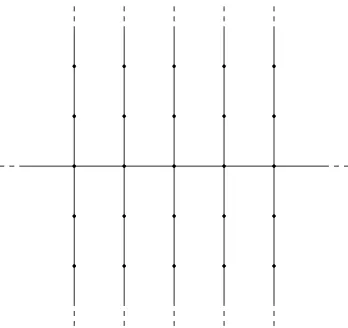
Figure 1: The 2-dimensional comb.
1
Introduction and main results
The 2-dimensional comb C2 is maybe the simplest example of inhomogeneous graph. It is
obtained fromZ2 by removing all horizontal edges off thex-axis (see Figure 1). Many features of the simple random walk on this graph has been matter of former investigations. Local limit theorems were first obtained by Weiss and Havlin (19) and then extended to higher dimensions by Gerl (10) and Cassi and Regina (4). More recently, Krishnapur and Peres (14) have shown that on C2 two independent walkers meet only finitely many times almost surely. This result,
together with the space-time asymptotic estimates obtained in (3) for the n-step transition probabilities, suggests that the walker spends most of the time on some tooth of the comb, that is moving along the vertical direction. Indeed in (3, Section 10), it has been remarked that, if
k/ngoes to zero with a certain speed, then p(2n) (2k,0),(0,0)/p(2n) (0,2k),(0,0) n−→→∞0. Moreover the results in (3) imply that there are no sub-Gaussian estimate of the transition probabilities on C2. Such estimates have been found on many graphs: by Jones (12) on the
2-dimensional Sierpi´nski graph, by Barlow and Bass (1) on the graphical Sierpi´nski carpet and on rather general graphs by Grigor’yan and Telcs ((11; 18)). These estimates involve three exponents which are usually associated to infinite graphs: the spectral dimension δs (which is by definition twice the exponent ofn−1 in local limit theorems), thefractal dimensionδf (which is the growth exponent) and the walk dimension δw (by definition the expected time until the first exit from the n–ball around the starting point is of order nδw). These dimensions are in
typical cases linked by the so-called Einstein relation: δsδw = 2δf (see Telcs (16; 17)). The first two dimensions are known forC2: δs = 3/2 andδf = 2. In this paper we computeδw= 2, thus showing that the relation does not hold for this graph.
In order to point out the different behaviour of the random walk along the two directions we analyze the asymptotic behaviour of the expected values of the horizontal and vertical distances reached by the walker innsteps. Different concepts of distance are considered: position aftern
steps, maximal deviation and maximal span (see Section 2 for the definitions).
the expected values of the “distances” (i.e. position, maximal deviation and maximal span) inn
steps for the simple random walk onZare of ordern1/2(the estimates for the maximal deviation
and maximal span were obtained by combinatorial methods by Panny and Prodinger in (15)). By comparison it is clear that the asymptotics coincide (to leading order) with the corresponding estimates for the vertical projection of the simple random walk onC2. We sketch the ideas of
the proof at the end of Section 2.
The behaviour of the horizontal projection of the random walk is less obvious: in Sections 3, 4 and 5 we prove that the expected values of the horizontal distance, of its maximal deviation and of its maximal span after nsteps are all of order n1/4 (the exact constants are determined in Theorem 3.1, Theorem 4.4 and Theorem 5.1 respectively).
The proofs are based on a Darboux type transfer theorem: we refer to (9, Corollary 2), but one may also refer to (2) and to the Hardy-Littlewood-Karamata theorem (see for instance (8)). This theorem (as far as we are concerned) claims that if
F(z) :=
∞
X
n=0
anzn z→1
− ∼ (1 C
−z)α, α6∈ {0,−1,−2, . . .},
and F(z) is analytic in some domain, with the exception ofz= 1, then
ann→∞∼
C
Γ(α)n α−1,
(byan∼bnwe mean that an/bnn→∞→ 1). Hence the aim of our computation is to determine an explicit expression of the generating functions of the sequences of expected values of the random variables we are interested in. This is done employing the combinatorial methods used by Panny and Prodinger in (15).
Since the notions of maximal deviation innsteps and of first exit time from a k-ball are closely related, we determine the walk dimension ofC2 in Section 4. This is again done by comparison
with the simple random walk onZ.
In Section 6 we deal with the limit of the process obtained dividing byn1/4 and byn1/2
respec-tively the continuous time interpolation of the horizontal and vertical projections of the position afternsteps. As one would expect the limit of the vertical component is the Brownian motion, while the limit of the horizontal component is less obvious (it is a Brownian motion indexed by the local time at 0 of the vertical component). This scaling limit is determined in Theorem 6.1. Finally, Section 7 is devoted to a discussion of the results, remarks and open questions.
2
Preliminaries and vertical estimates
The simple random walk on a graph is a sequence of random variables {Sn}n≥0, where Sn represents the position of the walker at timen, and if xandy are vertices which are neighbours then
p(x, y) :=P(Sn+1 =y|Sn=x) = 1
deg(x),
where deg(x) is the number of neighbours of x, otherwise p(x, y) = 0. In particular on C2 the
Givenx, y∈C2, let
p(n)(x, y) :=P(Sn=y|S0 =x), n≥0,
be the n-step transition probability from x to y and P(S0 = (0,0)) = 1. Recall that the
generating function of a sequence{an}n≥0is the power seriesPn≥0anzn; by definition the Green function associated to the random walk on a graph X is the family of generating functions of the sequences{p(n)(x, y)}n≥0,x, y∈X, that is
G(x, y|z) =X n≥0
p(n)(x, y)zn.
The Green function, with x= (0,0), on C2 can be written explicitly as (see (3))
G (0,0),(k, l)|z =
( 1
2G(z)(F1(z))|k|(F2(z))|l|, if l6= 0,
G(z)(F1(z))|k|, if l= 0,
where
G(z) =
√
2
p
1−z2+√1−z2;
F1(z) = 1 + √
1−z2−√2p1−z2+√1−z2
z ;
F2(z) =
1−√1−z2
z .
We refer to (21, Section 1.1) for more details on the random walks on graphs, transition proba-bilities and generating functions.
An interesting feature of a random walk is the distance reached inn steps. This distance may be defined as kSnk, the distance at time n from the starting point, k · k denoting a suitable norm. On C2 the choice is between the usual distance on the graph k(x, y)k1 = |x|+|y| and k(x, y)k∞= max{|x|,|y|}.
Other “distances” are the maximal deviation and the maximal span innsteps.
Definition 2.1. [a.]
1. The maximal deviation in n steps is defined as
Dn:= max{kSik: 0≤i≤n}.
2. The maximal span in nsteps is defined as
Mn:= max{kSi−Sjk: 0≤i, j≤n}.
When we need to stress the use of a particular norm k · k+, we use the notations Dn(k · k+)
and Mn(k · k+). In order to deal with the two components of the walk, we writeSn= (Snx, Sny) and benote byDxn and Dny the maximal deviations of the two processes {Sxn}n≥0 and {Sny}n≥0
(defined on Z) respectively. By Mx
0 1 2 3 −1
−2 −3
1/4 1/2
1/2 1/2
1/2 1/2
1/4 1/2 1/2
1/2 1/2
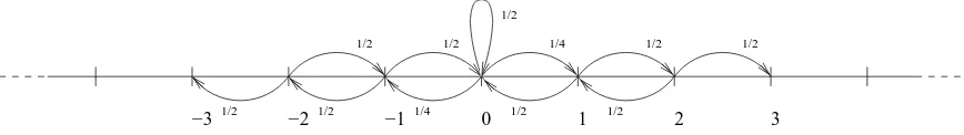
Figure 2: The vertical component of the simple random walk on C2.
Moreover we denote by| · |the usual norm onZ. It is worth noting that onZthe maximal span
may be equivalently defined as max{Si−Sj : 0≤i, j≤n}.
Among the issues of this paper are the asymptotics of E(|Sn∗|), E(Dn∗) and E(Mn∗), where ∗ is
eitherx ory.
Let us note that the asymptotics of the vertical component are already determined since they coincide (to leading order) with the corresponding estimates for the simple random walk on Z.
Indeed the vertical component of the simple random walk onC2(represented in Figure 2) differs
from the simple random walk onZonly in the presence of the loop at 0. Hence we may associate
to {Sny}n≥0 two sequences of random variables: {Yn′}n≥0 and {Ln}n≥0, such that {Yn′}n≥0 is a
simple random walk on Z, andLn is the number of loops performed by {Sny}n≥0 up to time n.
Thus Sny =Yn′ −En, where the error term En is the (random) sum of Ln iid random variables
Zi withP(Zi =±1) = 12. One easily proves that Enis negligible in all three estimates (for more details aboutY′
n and Ln see Section 6).
For the simple random walkYn′ onZ,E[|Yn′|]∼p2/π n1/2 may be obtained from the generating
function of the walk using the technique of Theorem 3.1, while the asymptotics of its maximal deviation,pπ/2n1/2, and of its maximal span,p8/π n1/2, may be found in (15) (Theorem 2.14 and Theorem 3.4 respectively). Thus the following result is obvious.
Theorem 2.2. [a.]
1. E[|Sny|]n→∞∼ q
2
πn1/2; 2. E[Dyn]n→∞∼ pπ
2n1/2;
3. E[Mny]n→∞∼ q
8
πn1/2.
3
Mean distance
The estimate ofE[|Snx|] is quite easy and may be considered as a warm-up for the use of generating
functions techniques.
Theorem 3.1.
E[|Snx|]n→∞∼ 1
23/4Γ(5/4)n 1/4.
Proof. Since for k6= 0,
P(|Snx|=k) = 2X
l∈Z
it is clear that (exchanging the order of summation)
∞
X
n=0
E[|Snx|]zn= 2
∞
X
k=1
kX
l∈Z
G (0,0),(k, l)|z.
By elementary computation one obtains
∞
X
n=0
E[|Sx
n|]zn=G(z)
F1(z)
(1−F1(z))2
1 1−F2(z)
z→1−
∼ 1
23/4(1−z)5/4.
Thus, applying (9, Corollary 2) we obtain the claim.
The following Corollary is now trivial.
Corollary 3.2. On C2, E[kSnk1] and E[kSnk∞] are both asymptotic, as n goes to infinity, to
q 2
πn1/2.
4
Mean maximal deviation and walk dimension
4.1 Maximal horizontal deviation
In order to compute the generating function of {E[Dnx]}n≥0, we first need an expression for
another generating function.
Lemma 4.1. Let h ∈ N, l ∈ {0, . . . , h}. The generating function of the sequence {P(Dxn≤h, Sxn=l)}
n≥0 is
ψh,l
1−√1−z2
2z
!
· 2(1− √
1−z2)
z(√1−z2−1 +z),
whereψh,l(z) is the generating function of the number of paths onZof lengthn, from0tol with
maximal deviation less or equal toh.
Proof. Note that the paths we are interested in have no bound on the vertical excursions. Thus
we may decompose the walk into its horizontal and vertical components, and consider each horizontal step as a vertical excursion (whose length might be zero) coming back to the origin plus a step along the horizontal direction.
Keeping this decomposition in mind, it is clear that the generating function of the sequence
{P(Dxn≤h, Sn= (l,0))}n≥0 is
ψh,l
zGe(0,0|z) 4
!
,
Moreover we must admit a final excursion from (l,0) to (l, j) for some j ∈ Z, that is we must
multiply by
E(z) :=Ge(0,0|z) + 2
∞
X
j=1 e
G(0, j|z),
and the generating function of{P(Dnx≤h, Snx =l)}
n≥0 is
ψh,l
zGe(0,0|z) 4
!
·E(z).
Using (21, Lemma 1.13) and reversibility (see (21, Section 1.2.A)), it is not difficult to compute
e
G(0,0|z) =
21−√1−z2
z2 ,
e
G(0, j|z) = 1
2Ge(0,0|z)
1−√1−z2
z
!j
, j6= 0.
The claim is obtained noting that
zGe(0,0|z)
4 =
1−√1−z2
2z ,
E(z) = 2(1−
√
1−z2)
z(√1−z2−1 +z).
Proposition 4.2.
∞
X
n=0
E[Dxn]zn= 21 + 6v
2+v4
(1−v)4 X
h≥1
vh
1 +v2h,
where v is such that
v
1 +v2 =
1−√1−z2
2z . (1)
Proof. Let ψh,l(z) be as in Lemma 4.1, and put ψh(z) = P|l|≤hψh,l(z). Then the generating
function of{P(Dnx≤h)}n≥0 is
Hh(z) :=ψh
1−√1−z2
2z
! ·
21−√1−z2
z(√1−z2−1 +z).
Thus we may write the generating function ofE[Dnx] as
∞
X
n=0 ∞
X
h=0
P(Dx
n> h)
!
zn=
∞
X
h=0
1
1−z −Hh(z)
An explicit expression for ψh has been determined by Panny and Prodinger in (15, Theorem 2.2):
ψh(w) =
(1 +v2)(1−vh+1)2 (1−v)2(1 +v2h+2),
where w=v/(1 +v2). By the definition of Hh(z) it is clear that the relation between z and v is set by equation (1). Then it is just a matter of computation to obtain
Hh(z) =
(1 + 6v2+v4)(1−vh+1)2 (1−v)4(1 +v2(h+1)) ,
1 1−z =
1 + 6v2+v4
(1−v)4 ,
whence, substituting in (2), the claim.
Lemma 4.3.
X
h≥1
vh 1 +v2h
v→1− ∼ 4(1π
−v).
Proof. The proof is quite standard, we report it here for completeness. Put v = e−t, g(w) =
e−w/(1 +e−2w) and consider
f(t) :=X h≥1
e−ht 1 +e−2ht =
X
h≥1
g(ht).
The Mellin transform of f is:
f∗(s) =
Z ∞
0 X
h≥1
g(ht)ts−1dt
=ζ(s)
Z ∞
0 X
λ≥0
(−1)λe−(2λ+1)wws−1dw,
whereζ(s) =Ph≥1h−s is the Riemann zeta function. The knowledge of the behaviour off∗(s)
in a neighbourhood of 1, will give us the behaviour of f(t) in a neighbourhood of 0. Substitute
y= (2λ+ 1)w to obtain
f∗(s) =ζ(s)κ(s)Γ(s),
whereκ(s) =Pλ≥0 (1+2(−1)λλ)s, and Γ(s) = R∞
0 e−yys−1dy is the gamma function. Since ass→1+
ζ(s) = 1
s−1+O(1), Γ(s) = 1 +O(s−1),
we are left with the computation of the asymptotic behaviour ofκ(s). We may write
κ(s) = 1
whereζ(s, a) =Ph≥0(a+h)−sis the Hurwitz zeta function. Thus using the expansion ofζ(s, a) forsclose to 1 (see (20, Formula 13.21)) we obtain
κ(s) = π
4 +O(s−1). Hence we get
f∗(s)s→1
+
∼ π
4(s−1). Applying (6, Theorem 1, p.115),
f(t)t→∼0+ π 4t,
which, substitutingt=−log(1−(1−v)), gives the claim.
Theorem 4.4.
E[Dxn]n→∞∼ 2
−7/4π
Γ(5/4)n
1/4.
Proof. By Proposition 4.2 and Lemma 4.3, it is clear that
X
n≥0
E[Dxn]zn v→∼1− 4π
(1−v)5. (3)
Choosing the solution v of equation (1) which is smaller than 1 when z is smaller than 1, and substituting it in (3) we obtain
∞
X
n=0
E[Dnx]zn z→∼1− 2
−7/4π
(1−z)5/4,
and (by (9, Corollary 2)) the claim.
Recalling Theorem 2.2, and the inequalities
Dny ≤ max
0≤i≤nkSik∞≤0max≤i≤nkSik1 ≤D x n+Dyn.
the following corollary is obvious.
Corollary 4.5. OnC2, bothE[Dn(k·k1)]andE[Dn(k·k∞)], asngoes to infinity, are asymptotic
topπ/2n1/2.
4.2 Walk dimension
The maximal deviation of a random walk is linked to the first exit time from a ball of radiusk. Indeed if we putTk= min{i:Si 6∈Bk}, where Bk is the ball of radiuskcentered in (0,0), then
(Dn≤k) = (Tk> n).
this choice will not affect the definition of the walk dimension, which, as we recalled in the introduction, is defined for a graphGasδw(G) =αifE[Tn] is of ordernα (andTn is computed with respect to the simple random walk onG).
By the results obtained so far it is clear that on C2, E[Tn] is of order n2, sinceδw(Z) = 2. It
is perhaps less obvious that the exact asymptotics aren2 and that this also holds when dealing withE[T∞
n ].
The first asymptotics are obtained by comparison with the simple random walk onZ: we sketch
here the derivation of the asymptotics of E[Tn(Z)] via generating functions techniques. The
behaviour of the latter sequence is well known, nevertheless we briefly report here a proof in order to give a hint as to how to proveE[Tn∞]∼n2.
Proposition 4.6. E[Tn]n→∞∼ n2 and E[T∞
n ] n→∞
∼ n2.
Proof. We write
E[Tn] =X
k≥0
P(Tn> k),
that is,E[Tn] = Θn(1), where Θn(z) is the generating function of the sequence{P(Tn> k)}k≥0= {P(max0≤i≤kkSik1 ≤ n)}k≥0. We claim that P(max0≤i≤kkSik1 ≤ n) = P(max0≤i≤k|Sei| ≤ n)
where {Sei}i≥0 is a suitable representation of the simple random walk on Z. Indeed it suffices
to consider the map that associates to each trajectory on C2 a trajectory on Z which jumps
fromj to j+ 1 whenever onC2 one of the two components increases and jumps from j toj−1
otherwise (i.e. when one of the components decreases).
The generating function of the number of paths onZof lengthk, with maximal deviation smaller or equal tonis Ψn(z) = (1+v
2)(1
−vn+1)2
(1−v)2(1+v2n+2) with the substitutionz=v/(1+v2), which was obtained
in Theorem 2.2 of (15). Thus
Θn(z) =
(1 +v2)(1 +v+· · ·+vn)2
(1 +v2n+2) (4)
with the substitutionz= 2v/(1 +v2). For z=v= 1 we get Θ
n(1) = (n+ 1)2.
The same methods used for E[Tn] apply to the evaluation of E[Tn∞] (one only has to carefully
decompose the walk much in the spirit of what was done in Lemma 4.1). The proof of this last estimate is omitted.
Corollary 4.7. The walk dimension of C2 is equal to2.
5
Mean maximal span
Theorem 5.1. E[Mnx]n→∞∼ 21/4
Γ(5/4)n1/4.
Proof. Letmx
n= max{Six : 0≤i≤n}. Then it is clear thatE[Mnx] = 2E[mxn]. Our first aim is to compute the generating function of{P(mx
n≤h)}n≥0, which we denote byΨeh(z). Then
e
Ψh(z) = lim k→∞
h
X
l=−k
e
where Ψeh,k;l(z) is the generating function of the probabilities of the n-step paths such that
−k≤Six ≤h for 0≤i≤n,Sn= (l,0) andSnx−1 6=l, whileE(z) was defined and computed in
Lemma 4.1. Let us note that Ψeh,k;l(z) = Ψh,k;l(zGe(0,0|z)/4), where Ψh,k;l(z) is the generating function of the number of the n-step paths onZ which stay in the interval between −k and h,
and end atl. The functions Ψh,k;l(w) are determined by the linear system used in (15, Theorem 4.1) to determine Ψh,k;0(w). Thus
Ψh,k;l(w) =
wlah−l−1(w)ak−1(w)
ah+k(w)
, ifl≥0,
Ψh,k;l(w) =
w−lah−1(w)ak+l−1(w)
ah+k(w)
, ifl≤ −1.
Then we put w = zGe(0,0|z)/4 = v/(1 +v2) and we obtain that (compare with the proof of Proposition 4.2)
lim k→∞
h
X
l=−k
e
Ψh,k;l(z) =
(1 +v2)(1−vh+1) (1−v)2 ,
E(z) = 1 + 6v
2+v4
(1 +v2)(1−v)2.
Then
e
Ψh(z) =
(1 + 6v2+v4)(1−vh+1)
(1−v)4 ,
∞
X
n=0
E[mxn]zn= 1 + 6v
2+v4
(1−v)4 X
h≥0
vh+1 z→∼1− 1
23/4(1−z)5/4,
whenceE[mx
n] n→∞
∼ 2−3/4n1/4/Γ(5/4) and we are done.
Corollary 5.2. OnC2, bothE[Mn(k·k1)]andE[Mn(k·k∞)], asngoes to infinity, are asymptotic
top8/π n1/2.
6
Scaling limits
In the preceding sections we have seen that the expected values of the distances (with various meanings of this word) reached in n steps are of order n1/4 for the horizontal direction and of order n1/2 for the vertical direction. These results lead us to a natural question: what is the
asymptotic behaviour of the process where the horizontal component of the position after n
steps is divided by n1/4 and the vertical component is divided by n1/2? Of course we have to make this question more precise.
In order to study the scaling of the process we choose a suitable realization for the sequence
{Sn}n≥0: let X = {Xn}n≥0 be a sequence of random variables representing a simple random
to Figure 2. ChooseX and Y to be independent and letX0=Y0 ≡0 almost surely. Moreover,
letLk be the number of loops performed byY up to time k, that is
Lk = k−1 X
i=0
1lYi=0,Yi+1=0.
Clearly, Sn = (XLn, Yn) is a realization of the position of the simple random walker on C2 at
time n. We are now able to define, by linear interpolation of the three discrete time processes
X, Y andL, a continuous time process (XLnt, Ynt).
Theorem 6.1.
XLnt 4
√
n , Ynt
√
n
t≥0
Law
−→WL0 t(B), Bt
t≥0, (5)
where W and B are two independent Brownian motions and L0t(B) is the local time at 0 ofB.
The theorem will be a consequence of Proposition 6.4 and Proposition 6.5. We introduce the following notion of convergence of stochastic processes (see Definition 2.2 of (5)).
Definition 6.2. A sequence of Rk-valued stochastic processes (Ztn;t ≥ 0)n≥0 converges to a
process (Zt;t≥0) in probability uniformly on compact intervals if for all t≥0, as n→ ∞
sup s≤tk
Zsn−Zsk−→P 0,
where k · k is a norm on Rk (for instance k · k1). We will briefly write
(Ztn;t≥0)−→U.P. (Zt;t≥0).
Since U.P. convergence of a vector is equivalent to U.P. convergence of its components and implies convergence in distribution, in order to prove Theorem 6.1 it will suffice to prove that each component in (5) U.P. converges to the corresponding limit.
The main idea is thatY and Lare not much different from, respectively, a simple random walk
Y′ onZand the processL′ which counts the visits ofY′ to 0. There is a natural correspondence
betweenY andY′, so let us defineY′ and some other auxiliary variables which will be needed in
the sequel. GivenY, letland N be the processes which respectively count its returns to 0 (not including the loops and counting time 0 as the first “return”) and the time spent not looping at 0. Namely, let l0 = 1, and lk = 1 +Pki=0−11lYi+1=0,Yi6=0 and Nk =
Pk−1
i=0 1lYi6=Yi+1 for k ≥1.
Clearly Nk=k−Lk. Moreover, note that fork≥1,
lXk−1
i=0
τi≤Lk≤ lk X
i=0
τi, (6)
whereτ ={τi}i≥0 is a suitable sequence of iid random variables with geometric distribution of
parameter 1/2. Now define a simple random walkY′onZbyYn=Y′
Nn. ThenL′k= Pk
i=01lY′
i=0
(L′ counts the visits at 0 or, equivalently, the returns to 0). We note that ln = L′Nn and
Lemma 6.3.
much different fromn. Indeed one can easily prove the first fact (for the distribution of (L′ 2n−1) see (7, Chapter III, Exercise 10)). By (6), the claim is a consequence of
Pln
By the strong law of large numbers and Slutzky’s theorem,
PL′
j be the number of visits to 0 before time
j of the random walk Ym′′ := Y′ is possible by the law of large numbers using the facts that L′′ and τe are independent and
Proposition 6.4.
Proof. Consider the processes Y′ and L′ defined before Lemma 6.3 and by interpolation define
the sequence of two-dimensional continuous time processes (√1
nYnt′ ,
by Theorem 3.1 of (5) we have that
To prove our statement, it suffices to show that these two properties hold:
(A) : are identically distributed, and maxk≤L⌊nt⌋
(9) it suffices to show that
1
√
The distribution of Mn is well known (see (7, Chapter III.7)), and it is easy to show that
Now, let us address to (B). We first note that we may consider a mapping between the number of steps taken by Y′ and the ones taken by Y. Indeed when Y′ has taken ⌊nt⌋ steps, then Y
has taken⌊nt⌋+Pi≤L′
⌊nt⌋τi steps (that is, ifY ′
⌊nt⌋= 0 we decide to count for Y all the loops it
performs after this last return to 0). Let us write
1
Now choose δ > 0. By independence of L′ and τ we have that the probability that maxk≤L′
The first term is smaller than δ if α and n are sufficiently large. As for the second term, it is clearly less or equal to
Observe that, by the law of large numbers, for any positive ε′ and δ there exists k0 =k0(ε′, δ)
Hence (11) is less or equal to
P
The first term clearly tends to 0 asngrows to infinity, while the second term is not larger than
δ+P
Using (8) and the definitions ofL′′ andτethereafter, we have thatPL
Choose α such that P
L′′⌊nε′⌋> α p
⌊nε′⌋ < δ for n sufficiently large, and then ε′ sufficiently
small such thatPP
i≤α√⌊nε′⌋τei > ε
larger than 1−δ. Hence, as in (12) we have that, forαandnsufficiently large andε′′ sufficiently small.
Proof. Clearly the statement may be rephrased as
X
Note that (writing L0
and both these summands tends U.P. to 0 (the first by Proposition 6.4). In order to show that
it suffices to prove that
P max probability may be written as
∞
can be made arbitrarily small ifnis picked large enough, while
Thus if δ > 0 is fixed, by choosing α sufficiently small we get P M
⌊nα⌋> ε√n
< δ if n is sufficiently large. This proves (A)U.P.→ 0.
Now note thatXn and L0s are independent, so we may think of X⌊nL0
whence (13). Thus, putting
7
Final remarks
The inhomogeneity of C2 results in the difference between the behaviour of the horizontal and
vertical components of the walk. Indeed while for any positive integerd the expected value of the distance from the origin of the simple random walker on Zd, aftern steps, is of order n1/2
(this may be easily proven via a conditioning argument, with respect to the proportions of time spent along each of thedmain directions), the expected value of the horizontal distance on C2
is of order n1/4, that is on this direction we have a subdiffusive behaviour.
The difference between the two projections of the walk is remarkable also when one properly rescales the process as we did in Section 6. Indeed although both components scale to a Brow-nian motion, the horizontal one is much slower (its clock is the local time at 0 of the vertical component).
Finally, also the failure of the Einstein relation on C2 is due to the inhomogeneity of this
particular graph. Indeed for strongly inhomogeneous graphs the growth exponent does not give an accurate description of the “fractal properties” of the graph (the assignment of the sameδf of
Z2 toC2 disregards the topology of the two structures). It seems that definingδf as the growth
exponent of the graph makes sense only for homogeneous graphs (likeZd) or self-similar graphs,
which have a clear fractal nature (like the Sierpi´nski graph). It is our opinion that the study of the sense in which a graph has a fractal nature and what is the proper definition of its fractal dimension should require further investigations.
Acknowledgments
I feel particularly indebted to Peter Grabner and Helmut Prodinger for raising the questions discussed in this paper and for the stimulating discussions during which they suggested the techniques used in Sections 3, 4 and 5. I would also like to thank Jean-Francois Le Gall for suggesting the limit of the rescaled process and giving me some precious hints.
References
[1] M.T. Barlow and R.F. Bass, (1999) Random walks on graphical Sierpi´nski carpets.
Ran-dom walks and discrete potential theory (Cortona, 1997), 26–55, Sympos. Math., XXXIX,
Cambridge Univ. Press, Cambridge. MR1802425
[2] E.A. Bender, (1974) Asymptotic methods in enumeration, SIAM Rev., 16, 485-515. MR0376369
[3] D. Bertacchi and F. Zucca, (2003) Uniform asymptotic estimates of transition probabilities on combs. J. Aust. Math. Soc. 75no.3, 325–353. MR2015321
[4] D. Cassi and S. Regina, (1992) Random walks on d-dimensional comb lattices. Modern
[5] A.S. Cherny, A.N. Shiryaev and M. Yor, (2002) Limit behaviour of the “horizontal-vertical” random walk and some extensions of the Donsker-Prokhorov invariance principle. Theory
Probab. Appl. 47no.3, 377–394. MR1975425
[6] G. Doetsch, (1956) Handbuch der Laplace-Transformation. Birkh¨auser Verlag, Basel-Stuttgart. MR0344808
[7] W. Feller, (1968)An Introduction to Probability Theory and Its Applications, vol. I 3rd ed., John Wiley and Sons, New York. MR0228020
[8] W. Feller, (1971) An Introduction to Probability Theory and Its Applications, vol. II 2nd ed., John Wiley and Sons, New York. MR0270403
[9] P. Flajolet and A. Odlyzko, (1990) Singularity analysis of generating functions. SIAM
J. Discrete Math. 3 no.2, 216–240. MR1039294
[10] P. Gerl, (1986) Natural spanning trees of Zd are recurrent. Discrete Math. 61 no. 2–3,
333–336. MR0855341
[11] A. Grigor’yan and A. Telcs, (2001) Sub-Gaussian estimates of heat kernels on infinite graphs.
Duke Math. J. 109 (2001) no.3, 451–510. MR1853353
[12] O.D. Jones, (1996) Transition probabilities for the simple random walk on the Sierpi´nski graph.Stochastic Process. Appl. 61, 4–69. MR1378848
[13] I. Karatzas and S. Shreve, (1991) Brownian motion and Stochastic Calculus, 2nd edition, Springer-Verlag, New York. MR1121940
[14] M. Krishnapur and Y. Peres, (2004) Recurrent graphs where two independent random walks collide finitely often. Electron. Comm. Prob. 9, 72–81. MR2081461
[15] W. Panny and H. Prodinger, (1985) The expected height of paths for several notions of height.Studia Sci. Math. Hungar. 20no.1-4, 119–132. MR0886012
[16] A. Telcs, (1990) Spectra of graphs and fractal dimensionsI.Probab. Theory Related Fields
85, 489–497. MR1061940
[17] A. Telcs, (1995) Spectra of graphs and fractal dimensionsII.,Probab. Theory Related Fields
8, 77–96. MR1308671
[18] A. Telcs, (2001) Local sub-Gaussian estimates on graphs, the strongly recurrent case.
Elec-tron. J. Probab.6 no.22, 1–33. MR1873299
[19] S. Havlin and G.H. Weiss, (1986) Some properties of a random walk on a comb structure.
Physica 134A, 474–482.
[20] E.T. Whittaker and G.N. Watson, (1962) A course of modern analysis. An introduction to the general theory of infinite processes and of analytic functions: with an account of
the principal transcendental functions. Fourth edition. Cambridge Univ. Press, New York.
MR0178117