Full Terms & Conditions of access and use can be found at
http://www.tandfonline.com/action/journalInformation?journalCode=ubes20
Download by: [Universitas Maritim Raja Ali Haji] Date: 12 January 2016, At: 23:41
Journal of Business & Economic Statistics
ISSN: 0735-0015 (Print) 1537-2707 (Online) Journal homepage: http://www.tandfonline.com/loi/ubes20
Long Swings in Exchange Rates
Franc Klaassen
To cite this article: Franc Klaassen (2005) Long Swings in Exchange Rates, Journal of Business & Economic Statistics, 23:1, 87-95, DOI: 10.1198/073500104000000505
To link to this article: http://dx.doi.org/10.1198/073500104000000505
View supplementary material
Published online: 01 Jan 2012.
Submit your article to this journal
Article views: 45
View related articles
Long Swings in Exchange Rates: Are They
Really in the Data?
Franc K
LAASSENDepartment of Economics, University of Amsterdam, Roetersstraat 11, 1018 WB, Amsterdam, The Netherlands (f.klaassen@uva.nl)
Several authors have reported evidence of long swings in U.S. dollar exchange rates by rejecting the random walk in favor of a Markov regime-switching model. We show that this evidence is not robust to an extension of the sample period. One should, however, not conclude that long swings are thus absent, because the tests may have insufficient power. A possible reason for this is the low data frequency, because existing tests are based on quarterly data, and we find that the power can be increased substantially by raising the data frequency. Indeed, weekly data reject the random walk, so we conclude that long swings are in the data. This conclusion is supported by significant superiority of regime switching over random walk out-of-sample forecasts of the direction of change.
KEY WORDS: Data frequency; Forecasting; Markov regime switching; Random walk; Testing; Unidentified parameters.
1. INTRODUCTION
Modeling exchange rates has been a main endeavor. Several structural models of exchange rate determination have been de-veloped, but their empirical validity is often questioned, espe-cially in the short run (MacDonald and Taylor 1992). Hence many researchers have used the random walk, particularly since Meese and Rogoff’s (1983) conclusion that random-walk fore-casts outperform those from structural exchange rate models.
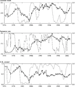
Nevertheless, the random walk remains unsatisfactory from an economic standpoint, because it ignores the impact of eco-nomic fundamentals. Moreover, time plots of exchange rates suggest some structural pattern. For instance, the thick lines in the three panels of Figure 1 (representing logarithms of weekly dollar prices of a German mark, Japanese yen, and U.K. pound from April 1974 to July 2003) indicate persistent appreciation and depreciation periods, that is, long swings.
But swings may also be just a pattern imposed by the eye on the realization of a random walk. To resolve the question whether long swings are a systematic part of exchange rates requires a formal test. The aim of this article is to do such a test using data on the aforementioned three dollar rates.
The outcome of the test not only will help understand the time path of exchange rates, but also is worthwhile for other reasons. For example, swings may originate from economic fundamentals. After all, if economic growth is relevant for ex-change rates, then business cycle differences between countries can lead to long swings in exchange rates. Moreover, changes in economic policy may affect the exchange rate–generating process (Lucas 1976). Kaminsky (1993), for example, showed theoretically that a change from a contractionary to an expan-sionary monetary policy regime increases the exchange rate de-preciation, resulting in long swings. Hence, knowing whether swings exist could guide future research on exchange rate de-termination.
To test for long swings, we use a Markov regime-switching model, introduced by Hamilton (1989) and used by many others thereafter. Engel and Hamilton (1990), Kaminsky (1993), Engel (1994), Evans and Lewis (1995), and Dewachter (1997) mod-eled long swings in exchange rates. Hamilton (1989), Hansen (1992, 1996), Goodwin (1993), Ghysels (1994), and Coe (2002)
used regime-switching models to analyze recessions and expan-sions in the U.S. business cycle, whereas Garcia and Perron (1996) and Ang and Bekaert (1998) model interest rates as a regime-switching process.
The Markov-switching model has two regimes (i.e., states) with potentially different mean exchange rate changes, presum-ably an appreciation regime and a depreciation regime. If the means are indeed different across both regimes, and if these “mean” regimes are persistent, then there exist long swings. If the means are the same across regimes, then the exchange rate follows a random walk (with drift). The test for long swings is therefore a test of the null hypothesis that the means are equal across regimes against the alternative of different means and persistent regimes.
Several authors have already tested for long swings (e.g., Engel and Hamilton 1990; Engel 1994). Using quarterly data up to about 1986, they concluded that long swings exist.
Given that we now have more data, we can redo their tests with quarterly data up to 2003. The results are changed in the sense that there is no longer convincing evidence of long swings. This lack of evidence is confirmed by applying Hansen’s (1992, 1996) testing methodology, which is particu-larly designed for testing null hypotheses such as the one given earlier in a Markov-switching model.
The lack of evidence is no proof of the absence of long swings, however; it may be due to insufficient test power. A pos-sible reason for this is the data frequency; even if swings exist and last for some quarters, sampling at the quarterly frequency may result in too few observations per swing to enable one to distinguish the swings from a random walk. We confirm this reasoning by a Monte Carlo simulation study.
To obtain a more powerful test for long swings, we thus in-crease the data frequency of the three observed dollar rates from quarterly to monthly and then to weekly. Applying Hansen’s test yields our final answer concerning the existence of long swings in exchange rates.
© 2005 American Statistical Association Journal of Business & Economic Statistics January 2005, Vol. 23, No. 1 DOI 10.1198/073500104000000505
87
88 Journal of Business & Economic Statistics, January 2005
Figure 1. Logarithm of Exchange Rates (dollars per foreign cur-rency, thick line, left axis) and Smoothed Regime Probabilities (thin line, right axis).
In the next section we describe the regime-switching model and the procedure to test for long swings. In Section 3 we give the empirical results. There we actually test for the existence of long swings and examine the role of the data frequency. We also present the estimation results and an out-of-sample fore-casting study that compares long swings to random walk based forecasts. We conclude in Section 4.
2. MODEL AND TEST FOR LONG SWINGS
2.1 Regime-Switching Model
Because we want to use a regime-switching model for weekly exchange rates, we have to generalize the basic Hamilton (1989) regime-switching model to incorporate the high-frequency features of exchange rates, particularly condi-tional heteroscedasticity and leptokurtosis of the innovation. Therefore, we introduce an extended regime-switching model that includes a generalized autoregressive conditional het-eroscedasticity (GARCH) model for the variance (see Bollerslev, Chou, and Kroner 1992 for an overview of GARCH) and at-distribution for the innovation. The model consists of four elements: the mean, regime process, variance, and distri-bution. We discuss these elements subsequently and relate our specification to the one given by Engel and Hamilton (1990).
Let St denote the logarithm of the spot exchange rate at
timet, that is, the domestic currency price of one unit of for-eign currency. We concentrate on the exchange rate change
st=100(St−St−1), so thatst is the percentage depreciation of
the domestic currency from timet−1 tot.
The mean ofst depends on which (unobservable) regime the
process is in. Following Engel and Hamilton (1990), we assume that there are two regimes. Letrt∈ {1,2}denote the regime at
timet. Within this regime, the mean exchange rate depreciation isµrt, and we identify the first regime as the low mean regime,
µ1≤µ2.
We assume that within each regime the mean conditional on previous exchange rate changes is constant over time, although it is possible to allow for autoregressive terms, among other things. Hence the mean equation is
st=µrt+εt, (1)
where the expectation of the innovation εt is 0 conditional
on the current regime rt and the information set of the
data-generating process. This set consists of two parts. The first part,It−1=(st−1,st−2, . . . ), denotes the information observed by the econometrician; the second part,rt−1, is the regime
path (rt−1,rt−2, . . . ), which is not observed. We thus get
E{εt|It−1,rt} =0. Using the subscriptt−1 below an
opera-tor (probability, expectation, or variance) as shorthand notation for conditioning onIt−1, this givesEt−1{εt|rt} =0.
The persistence of both regimes depends on the regime-staying probabilities. Letpt−1(rt|rt−1)denote the probability of going to regimert at timetconditional on the information set
of the data-generating process. Following Engel and Hamilton (1990), we assume thatrtfollows a first-order Markov process
with constant staying probabilities, so that
pt−1(rt|rt−1)=p(rt|rt−1)=
p11, ifrt=rt−1=1
p22, ifrt=rt−1=2. (2) The mean and regime processes just described are able to capture long swings in exchange rates. After all, if µ1< µ2 and ifp11andp22are high, then being in the first regime leads to probably a long period of appreciation (assuming, for sim-plicity, thatµ1<0) and, after a switch to the second regime, to probably a long period of depreciation (assuming thatµ2>0). Hence there are long swings. Note, however, that the model does not impose the existence of swings; we do allow for µ1=µ2, so that exchange rates can have a constant mean, as in the random walk with drift.
When specifying the conditional variance,Vt−1{εt|rt}, Engel
and Hamilton (1990) assumed that this variance is constant within a regime. This may well be fine for the quarterly data of Engel and Hamilton, but is problematic for our weekly data. After all, if mean regimes are persistent (a few years according to Engel and Hamilton), then the variance is also constant for a long time. This is particularly problematic for high-frequency data, because it is well known that there is conditional het-eroscedasticity. Moreover, if the model with constant regime-specific variances is estimated with weekly data, then it may well be that the regimes are exploited to capture the strong con-ditional heteroscedasticity instead of the long swings in which we are interested. This may yield a significant test for the exis-tence of two regimes, even if there are no long swings.
The second feature of the Engel and Hamilton (1990) vari-ance specification is that the varivari-ance is different across the two mean regimes. As the authors admitted, the perfect dependence between mean and variance can be problematic. For instance, if the appreciation regime is associated with high volatility, then
a period of unusual volatility can force the process into this ap-preciation regime, even when the currency is actually depreci-ating. Moreover, economists are not convinced that there is any relation between the mean and the variance of exchange rates (see, e.g., Engle, Ito, and Lin 1990).
As a solution for both issues, we disconnect the variance from the regime process, which thus is completely focused at the long swings. For the variance specification, we use the pop-ular GARCH approach.
A direct application of the standard GARCH(1,1)formula in our regime-switching model would define the conditional error variance as
Vt−1{εt|rt} =ω+αε2t−1+βVt−2{εt−1|rt−1}. (3) This specification appears practically infeasible when estimat-ing the model, however. In buildestimat-ing the sample log-likelihood, the econometrician first uses (1) to express the unobservedεt2−1 in terms of the conditioning variables byε2t−1=(st−1−µrt−1) quently, the conditional variance in (3) depends on the entire sequence of regimes up to time t−1. Because the number of possible combinations grows exponentially witht−1, this leads to an enormous number of regime paths tot−1. The econome-trician, who does not observe regimes, must integrate out all possible regime paths. This renders estimation intractable.
To avoid this path-dependency problem, it is interesting to realize that the same problem also hampered the application of regime-switching GARCH models, where the conditional vari-ance depends on the varivari-ance regime that the process is in and where the conditional variance within each variance regime is governed by a GARCH process. For such models, Gray (1996) introduced a way to remove the path dependence from the like-lihood.
We apply the basic idea behind that technique to solve the problem in our regime-switching mean model as well. That is, we directly average out the regimes rt−1 in the source of the path dependence,εt2−1=(st−1−µrt−1)
2, instead of only in the likelihood. This removes the regime dependence ofVt−1{εt|rt}.
To average out the regimes, we follow Klaassen’s (2002) ap-proach, because it improves on Gray’s method. That is, we use the observed informationIt−1, so thatVt−1{εt|rt}becomes
The fourth and final element of the regime-switching model concerns the conditional distribution of exchange rate changes. Engel and Hamilton (1990) chose a normal distribution for their quarterly series. However, to allow for extra leptokurtosis in our weekly data, we follow other authors by taking at-distribution (see Bollerslev, Chou, and Kroner 1992). It has ν degrees of freedom, mean 0, and varianceVt−1{εt},
εt|It−1,rt∼t(ν,0,Vt−1{εt}). (5)
Equations (1), (2), (4), and (5) describe the complete regime-switching model. We estimate it by maximum likelihood using a sample ofstfort=1, . . . ,T. The likelihood function, which
has a convenient recursive structure, can be derived in a simi-lar way as done by Klaassen (2002). To start up the recursive process, we set the required variables equal to their expectation without conditioning on observable informationIt−1.
2.2 Testing Procedure for Long Swings
The central feature of the model presented in the previous section is the allowance for two persistent regimes with differ-ent mean depreciations,µ1 andµ2, because these are able to capture long swings. Hence, to test for the existence of long swings, we test for the existence of such regimes. More for-mally, we test the null hypothesis of a single-regime model (µ1=µ2)—that is, the random walk with drift—against the regime-switching model of Section 2.1. In this section we set out the testing procedure; the empirical outcomes follow in the next section.
Testing the null restrictionµ1=µ2 is not straightforward. For instance, under the null there is in fact only one regime that governs the exchange rate, so that the regime-staying prob-abilitiesp11 andp22 are not identified (see Hansen 1992 for a discussion of other problems involved). This makes the asymp-totic distribution of the usual tests (likelihood ratio, Wald and Lagrange multiplier) no longer chi-squared (Hansen 1992).
Garcia (1998) proposed one way to overcome the problems. He derived the asymptotic distribution of the likelihood ratio test for several variants of the regime-switching model. How-ever, the model of Section 2.1, with the GARCH-based vari-ance andt-distribution for the innovation, was not included in Garcia’s article.
A generally applicable solution for the aforementioned test-ing problems was given by Hansen (1992, 1996). His ap-proach can be summarized as follows. The null restriction is equivalent to µ2−µ1=0. Under this null, p11 and p22 are not identified. The other parameters(µ1, σ2, α, β, ν)are iden-tified, however. Hansen proposed considering a fixed value for (µ2 −µ1,p11,p22). For this point, maximize the log-likelihood across the other five parameters; that is, concentrate out(µ1, σ2, α, β, ν). Subtracting the log-likelihood under the null and dividing this difference by its standard deviation yields the standardized likelihood ratio for the(µ2−µ1,p11,p22) un-der consiun-deration. Hansen’s test statisticLR∗is the supremum of these standardized likelihood ratios over all parameter com-binations(µ2−µ1,p11,p22)possible under the alternative. In practice, Hansen suggested taking the supremum over a finite grid of parameter combinations. The asymptoticpvalue ofLR∗
is not known by itself, but Hansen showed that it is smaller than or equal to the asymptoticpvalue using the distribution of another variable. He advised using this upper bound, although it makes the test conservative (i.e., too few rejections of the null). He also explained how the bound can be approximated via simulation. Finally, thepvalue bound depends on a band-width numberM, and Hansen suggested computing thepvalue for differentM(see Hansen 1996 for details).
In this article we follow Hansen’s method. Details on the im-plementation are given in the next section.
90 Journal of Business & Economic Statistics, January 2005
3. EMPIRICAL RESULTS
In this section we use the regime-switching model and the testing apparatus developed earlier to address the central ques-tion of this article—whether long swings really exist. First, we describe the data. Then we investigate existing tests for long swings. In Section 3.3 we perform our own test. After that, we analyze the estimates of the regime-switching model. In Sec-tion 3.5 we examine whether taking the long swings into ac-count leads to better out-of-sample exchange rate forecasts than those generated by the random-walk model.
3.1 Data
We use three U.S. dollar exchange rates, namely, the dol-lar vis-à-vis the German mark, the Japanese yen, and the U.K. pound. We chose these exchange rates because of their impor-tant role on foreign exchange markets and because they be-have relatively independently, for instance, compared to several dollar–EMS exchange rates. We have weekly data on exchange rate levels over the post–Bretton Woods period from April 2, 1974 to June 17, 2003; for the euro period, the German mark rates have been derived from the dollar/euro rates and the of-ficial mark/euro conversion rate. This givesT =1,524 obser-vations of the percentage dollar depreciations,st. These were
obtained from Datastream.
The thick lines in the three panels in Figure 1 show the be-havior of the logarithm of the three exchange ratesSt over the
sample period. At first sight, exchange rates indeed seem to be characterized by long swings. However, this graphical sugges-tion of course provides no formal evidence, because the long swings may be only a pattern imposed by the eye on the real-ization of a random walk. Hence we need a test.
3.2 Existing Tests for Long Swings
As explained in Section 2.2, testing for long swings is not straightforward. For instance, the regime-staying probabil-ities are not identified under the random-walk null hypothesis (a single-regime model), which makes the asymptotic distrib-ution of conventional tests no longer chi-squared. Several au-thors, including Engel and Hamilton (1990) and Engel (1994), circumvented the testing problems by introducing an auxiliary assumption to nevertheless be able to test for long swings. In this section we describe their approach and investigate the ro-bustness of their results to an extension of their sample period. Following their work, here we use quarterly data, obtained by elimination from the weekly level series described earlier.
The Engel and Hamilton (1990) approach, also followed by Engel (1994), is embedded in a Markov regime-switching model where the exchange rate change is normally distributed with mean µ1 and variance σ12 in the first regime and nor-mally distributed withµ2andσ22in the second regime, where (µ1, σ12)=(µ2, σ22). The model thus imposes that there are al-ways two regimes. This is the auxiliary assumption that the authors made to circumvent the testing problems mentioned earlier, which originated from the allowance for one regime.
Those authors used two tests for the existence of long swings. The first test is based on the fact that there are no long swings
if the two regimes have the same mean. The test thus concerns the null hypothesisµ1=µ2against the alternativeµ1=µ2.
The second Engel and Hamilton test investigates whether the regimes are persistent in the sense that the probability of being in a regime depends on the previous regime. If this is not the case, then the probability of staying in the first regime equals the probability of switching from the second to the first regime, so that there are no long swings. Hence they testp11=1−p22 versusp11=1−p22.
For both tests, the authors used the conventional likelihood ratio test with 5% critical value 3.84. We use the same signif-icance level throughout this article. Because the existence of long swings implies that bothµ1=µ2andp11=1−p22, only a rejection of both tests is evidence in favor of long swings.
We first compute both tests using similar data as used by Engel and Hamilton (1990) and Engel (1994), that is, the 1974:II–1986:IV subsample of our dataset. The likelihood ra-tios for theµ1=µ2andp11=1−p22tests are (3.15, 3.07) for Germany, (6.86, 4.35) for Japan, and (9.43 , 8.01) for the U.K. The results point at the existence of long swings and thereby corroborate the conclusion of Engel and Hamilton (1990) and Engel (1994).
Now we extend the data range by including 1987:I–2003:II. The likelihood ratios become (3.23, 1.04), (7.95, 2.73), and (3.31, 17.99), so that there is no longer evidence of long swings, except perhaps some indication for the U.K. For instance, the estimates for Japan, whereµ1=µ2is rejected butp11=1−p22 is not, reveal that the estimated regime-staying probabilityp11 is .441, implying that the low mean regime is short-lived instead of persistent, so that the estimates do not point to long swings.
We conclude that existing evidence of long swings depends on the sample period. Prolonging the data range no longer yields convincing evidence of long swings.
3.3 Long Swings in Exchange Rates: Are They Really in the Data?
As indicated in Section 1, the lack of evidence of long swings from quarterly data may be caused by the low data frequency. Therefore, in this section we analyze the effect of increasing the data frequency for the test outcome. To take account of the po-tential conditional heteroscedasticity and leptokurtosis, we re-turn to the model of Section 2.1. We use Hansen’s (1992, 1996) testing methodology described in Section 2.2, so that we do not have to make the auxiliary assumption that there undoubt-edly exist two regimes as in the previous section. To get fur-ther insight into the test, we first apply it to the same quarterly data as used in the previous section. After that we increase the frequency, so as to derive our final answer to the question of whether long swings exist.
3.3.1 Quarterly Data. As usual for quarterly data, we find no evidence of conditional heteroscedasticity and nonnormality. Hence, for the sake of parsimony, in this section we consider the model of Section 2.1 restricted byα=β =0 andν= ∞. We test the null hypothesisµ1=µ2, so the null model is the random walk with drift.
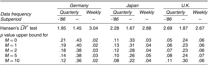
Because Hansen’s test is computed in practice by maxi-mizing the standardized likelihood ratio over a grid of(µ2− µ1,p11,p22), we first have to choose such a grid. This requires specification of the parameter space for these coefficients un-der the alternative hypothesis of long swings. Hence, what val-ues for (µ2−µ1,p11,p22)are reasonable in the case of long swings? We think that for the countries under consideration reasonable long appreciation and depreciation swings are not more than about 10 percentage points different on a quarterly basis, so thatµ2−µ1should be at most 10. We take the grid µ2−µ1∈ {.5,1,2, . . . ,10}.
The grid for the regime-staying probabilitiesp11 andp22 is based on what degree of persistence in swings is considered “long.” One usually thinks in terms of quarters or even years. Therefore, we assume that swings are called “long” if they last for at least, say, two quarters. Because the expected duration of a regime r is (1−prr)−1 (see Hamilton 1989), this
con-dition implies thatprr≥.5. However, if both p11 andp22 are small, thenp11+p22 is close to 1, which implies that the cur-rent regime is almost independent of the previous regime. This is in contrast with the idea of long swings. We therefore impose the extra restriction thatp11+p22is at least 1.2, say. The grid is
p11,p22∈ {.50, .55, .60, . . ., .95}such thatp11+p22≥1.2. The total number of grid points(µ2−µ1,p11,p22)is 990. The pre-cise grid choice is inevitably arbitrary. For many Hansen tests in this article, we thus have experimented with other grids. The results from those grids are essentially the same.
Table 1 presents the test results. The first column for each country reports them for the series from 1974:II–1986:IV, sim-ilar to the data used by Engel and Hamilton (1990) and Engel (1994). The Hansen statisticLR∗is 1.95 for Germany, 2.28 for Japan, and 2.69 for the U.K. The p value upper bounds are presented for different bandwidth parametersMand are based on 10,000 simulations. The bounds are above the level of 5%. Extending the sample period by including data from 1987:I– 2003:II raises the bounds even further. Hence we again find no evidence of long swings in quarterly data.
3.3.2 The Relevance of Data Frequency for Test Power.
The inability to reject the random walk may be caused by the absence of long swings. However, it may also be due to a lack of
power of the tests in a situation where swings are present. One possible reason for this is that the data frequency is too low. Af-ter all, even if swings are part of the exchange rate–generating process and last for some quarters, a sample of quarterly data may result in too few observations per swing to enable one to distinguish the swings from a random walk. Although this argu-ment may sound intuitively appealing, there is no direct support for it yet. Therefore, we explore that idea in this section.
The most closely related work is that of Coe (2002), who performed a Monte Carlo experiment to compute the power of Garcia’s (1998) test for the presence of regimes in a ho-moscedastic normal model. He first took estimates based on annual gross domestic product (GDP) data over 95 years as true parameter values for the Monte Carlo simulations of the regime-switching model. Then he repeated the study using esti-mates from quarterly GDP data over 37 years. Although Coe’s focus is not on the relevance of data frequency for test power, he did report an interesting result for the present article, that is, he found a power of .48 for datasets containing 100 observations based on the annual estimates and a power of .89 for datasets of 400 observations generated from the quarterly estimates. This gain in power may come from an increase in data frequency for a fixed time span. However, because the underlying annual and quarterly estimates are essentially different, so that the simu-lated annual series are not simply the time-aggregated versions of the simulated quarterly series, the actual contribution of the increase in data frequency to the gain in power is not clear. In addition, the impact of conditional heteroscedasticity and ex-cess kurtosis cannot be inferred.
The relevance of data frequency for test power has received considerably more attention in the literature on unit root tests. The common idea is that a longer span of the data is more im-portant than a higher frequency to increase the power, but that a higher frequency for a given time span can also provide signif-icant improvements in the finite-sample power (Maddala and Kim 1998, p. 130). The latter part, which is the relevant one for this article because we have a fixed time span, is based on homoscedastic normal processes, as used by Choi and Cheung (1995), among others.
Table 1. Tests for Existence of Long Swings in Exchange Rates
Germany Japan U.K.
Data frequency Subperiod
Quarterly Weekly Quarterly Weekly Quarterly Weekly -’86 – – -’86 – – -’86 – –
Hansen’sLR∗test 1.95 1.45 3.04 2.28 1.67 2.88 2.69 1.87 2.67
pvalue upper bound for
M=0 .21 .43 .02 .11 .33 .03 .05 .24 .06
M=1 .19 .40 .02 .13 .31 .04 .06 .23 .06
M=2 .18 .38 .03 .12 .28 .04 .07 .23 .06
M=5 .14 .38 .03 .10 .26 .05 .08 .24 .07
M=10 .12 .36 .02 .08 .22 .04 .11 .30 .06 NOTE: The test for long swings is a test of the null hypothesis of the random walk against the alternative of the regime-switching model of Section 2.1, which contains the null as the special caseµ1=µ2. For the quarterly frequency, both models have been restricted by imposing conditional homoscedasticity (α=β=0) and normality (ν−1=0).
The left column for the quarterly frequency uses data only through 1986:IV, that is, similar data as used by Engel and Hamilton (1990) and Engel (1994).
TheLR∗statistic is based on Hansen’s (1992,1996) method. Hence the upper bounds for thepvalues may depend on a bandwidth parameterM; the bounds are based on 10,000 simulations. For the quarterly data, the grid isµ2−µ1∈ {.5, 1.0, 2.0, . . . , 10.0}and
p11,p22∈ {.50, .55, .60, . . . , .95}, such thatp11+p22≥1.2, a total of 990 points. For the weekly data, the grid isµ2−µ1∈ {.01, .10, .20, . . . , 1.00}andp11,p22∈ {.950, .955, . . . , .995, .999}, a total of 1,331 points.
The required CPU times on a Pentium 733 computer are .2, .5, and 15 hours for the three columns per country.
92 Journal of Business & Economic Statistics, January 2005
There is also recent evidence that for conditionally het-eroscedastic and leptokurtic processes, the power of unit root tests increases substantially if one explicitly accounts for both features (Seo 1999). Because they can usually be captured with high-frequency data but not with low-frequency data, the result suggests a second reason why increasing the data frequency can lead to improvements in the power of unit root tests.
Because in this article we examine exchange rates, which have conditional heteroscedasticity and excess kurtosis in high-frequency data, and because our testing approach can account for this, the results from the unit root literature suggest that in-creasing the data frequency may indeed improve the power of long swings tests, as argued earlier.
To further support this claim, we perform a Monte Carlo experiment. We generate a sample of 1,000 exchange rate changes st that exhibit long swings. As the data-generating
process we use the GARCH-tregime-switching model of Sec-tion 2.1 with parameters similar to the estimates for weekly data discussed later (µ1= −.2, µ2=.2,p11=.98,p22=.98, σ2=1, α=.1, β=.85, ν=5); the data-generating process is initialized by regimer1=1 with probability .5 and by the varianceV0{ε1} =σ2. We call this the high-frequency sample. We carry out Hansen’s test forµ1=µ2taking account of the GARCH-tfeatures in the data and using the grid{.1, .2, . . . , .8}
forµ2−µ1and{.96, .97, .98, .99}forp11 andp22. Note that the number of grid points, 128, is much less than that used for the real data analyzes, because we want to limit the computer time for the Monte Carlo. (For 128 points, it already takes sev-eral days per parameter combination.) We have experimented with denser grids and found similar results.
Next we derive the low-frequency sample by dividing the high-frequency sample in groups of 10 consecutive exchange rate changes and adding up the changes, so that the low-frequency sample contains 100 observations. Because there ap-pears to be no evidence of GARCH-teffects in this sample, we apply Hansen’s test under homoscedasticity and normality. The grid forµ2−µ1is{1,2, . . . ,8}, and the grid forp11andp22is
{.6, .7, .8, .9}.
The foregoing procedure is repeated 500 times. The power is estimated by the relative frequency of rejections at the 5% nom-inal size using the bandwidth parameterM=10 for Hansen’s test.
The estimated power using low-frequency data turns out to be .27. For the high-frequency data it is .91. Hence the power improves considerably when the frequency is increased. This conclusion appears robust when experimenting with other Monte Carlo designs (various parameter values and grids), al-though the magnitude of the power improvement depends on the specific setup.
The results in the unit root literature as discussed earlier sug-gest that the gain in power originates from two sources, namely the increase in frequency for a homoscedastic normal data-generating process and the fact that only with high-frequency data one can account for conditional heteroscedasticity and lep-tokurtosis in the data-generating process. To examine to what extent this is true for long swings tests, we repeat the simula-tion study but now without the GARCH-teffects, that is, with α=β=0 andν= ∞. The low-frequency power becomes .36, and the high-frequency power becomes .62. Hence, from the to-tal gain of .64, we attribute .26 to the increase in frequency for
homoscedastic normal processes and .38 to the fact that high-frequency data allows one to capture conditional heteroscedas-ticity and excess kurtosis.
The gain in power may reflect that the actual size of the test using high-frequency data is much higher than for low-frequency data. To study this, we redo the original Monte Carlo but now withµ1=µ2=0 for the data-generating process. The size for the low-frequency data is estimated as .014, and that for the high-frequency is estimated as .006. Hence the concern just mentioned is not supported empirically.
The fact that both sizes are lower than the nominal size of .05 reflects the conservativeness of Hansen’s bound-based pro-cedure. The extent of conservativeness here may seem to con-tradict Hansen’s (1992) conclusion that the conservativeness is small for his application. However, concentrating on the high frequency, if we take a similar setup as done by Hansen (1992) by using a homoscedastic normal data-generating process (α=
β =0 and ν= ∞) and widening the grid for p11 andp22 to
{.1, .3, .5, .7, .9}, keeping the other elements the same, then the size becomes .04, in line with Hansen’s finding. Hence the lower size in our original setup is caused by the characteristics of that setup. Further analysis reveals that the GARCH effects, thet-distribution, and the narrower grid are all relevant, because adding either one of them to the Hansen-type setup already re-duces the size.
3.3.3 Weekly Data. The positive effect of data frequency on test power suggests redoing the long swings test for the three dollar exchange rates using a greater-than-quarterly frequency. We first increase the data frequency to monthly, but the tests remain insignificant.
Then we use weekly data. The grid choice is based on similar arguments as in Section 3.3.1, which leads to µ2− µ1 ∈ {.01, .10, .20, . . .,1.00} and p11,p22 ∈ {.950, .955, . . ., .995, .999}, in total 1,331 grid points. As Table 1 shows, the
p value upper bounds now yield evidence of the existence of long swings, particularly if one realizes that the test is conserv-ative, so that the truepvalues are smaller.
Our final conclusion is thus that the data really suggest that long swings exist. The previous inability to find long swings us-ing quarterly data is due not to the absence of swus-ings but rather to statistical reasons; the low data frequency leads to too few ob-servations per swing to enable one to significantly distinguish long swings from a single-regime process. Weekly data give the test enough power.
3.4 Estimation Results
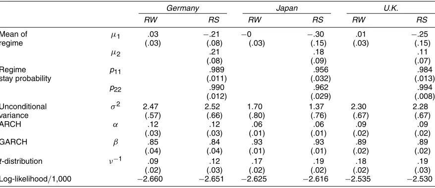
We now present the estimation results for the regime-switching model and, for comparison, the results for the ran-dom walk, all for the weekly data. For Germany, we add a first-order autoregressive term to mean equation (1), so that the mean equation for Germany isst=µrt+θ (st−1−µrt−1)+εt instead of (1).
As shown in Table 2, all three exchange rates are charac-terized by an appreciation swing (µ1<0) and a depreciation swing (µ2>0). The strong persistence of these swings is rep-resented by the large regime-staying probabilitiesp11andp22. Conditional homoscedasticity and conditional normality are
Table 2. Estimation Results
Germany Japan U.K.
RW RS RW RS RW RS
Mean of µ1 .03 −.21 −0 −.30 .01 −.25
regime (.03) (.08) (.03) (.15) (.03) (.15)
µ2 .21 .18 .11
(.08) (.09) (.07)
Regime p11 .989 .956 .984
stay probability (.011) (.032) (.013)
p22 .990 .962 .994
(.012) (.029) (.008)
Unconditional σ2 2.47 2.52 1.70 1.37 2.30 2.28
variance (.57) (.66) (.80) (.76) (.67) (.67)
ARCH α .12 .12 .06 .06 .09 .09
(.03) (.03) (.01) (.01) (.02) (.02)
GARCH β .85 .84 .93 .93 .89 .89
(.04) (.04) (.01) (.01) (.02) (.02)
t-distribution ν−1 .09 .12 .17 .19 .18 .19
(.02) (.03) (.02) (.02) (.02) (.03)
Log-likelihood/1,000 −2.660 −2.651 −2.625 −2.616 −2.535 −2.530
NOTE: Standard errors are in parentheses.
RW denotes the random walk, and RS the regime-switching model of Section 2.1. For Germany, however, the regime-switching model is extended by a first-order autoregressive term to correct for some short-term serial correlation; the estimate for the autoregressive parameter is .05 (.03).
We report the inverse of the degrees of freedom of thet-distribution, because testing for conditional normality then boils down to simply testing whetherν−1differs from 0.
strongly rejected. Finally, the autocorrelations of the normal-ized residuals and their squares (not reported) support the model specification.
To get a better idea about the degree of regime persistence that the staying probabilities imply, we first compute the ex-pected duration of a regime r, which is (1−prr)−1. The
av-erage estimates ofp11 andp22 imply an expected duration of about a year for both regimes. These are comparable to those of Engel and Hamilton (1990), despite the fact that our estimates are based on weekly data instead of quarterly data.
A second way to examine the persistence of regimes is by inspecting smoothed regime probabilities. The smoothed probability of a particular regime at time t is the probability that the process was in that regime at time t using the com-plete datasetIT (see Klaassen 2002 for its computation). The
smoothed regime probabilities, plotted in Figure 1, confirm that regimes are persistent.
3.5 Forecasting Performance
Given the existence of long swings, a natural question is whether this can be exploited to forecast exchange rates. There-fore, in this section we compare the out-of-sample forecast quality of the regime-switching models estimated in Section 3.4 to the random walk.
The forecast under consideration isEt−1{Sτ}, the expected exchange rate at some future time τ using information at timet−1. The forecasts for the regime-switching model are computed using similar formulas as used by Klaassen (2002); for the random walk, the forecasts are the previous exchange rate St−1 plus a drift term. We examine three horizons, τ − (t−1), namely 1 week, 1 month (4 weeks), and 1 quarter (13 weeks). There are 1,524 out-of-sample forecasts, resulting from the procedure described in the note for Table 3.
We evaluate the forecasts in two ways. First, we examine how well a forecastEt−1{Sτ}predicts the level of the future ex-change rateSτ. This is point prediction. As usual, we take the
mean squared error (MSE) criterion,T1Tt=1(Sτ−Et−1{Sτ})2. The left panel of Table 3 reports the MSE of the regime-switching model (left column for each country) and the MSE difference with respect to the random walk (right column). Their standard errors are heteroscedasticity and autocorrelation consistent (see the note in Table 3).
Table 3 shows that the regime-switching model does not out-perform the random walk in terms of MSE. This corroborates the findings of Engel (1994), but it contrasts with the conclu-sion of Engel and Hamilton (1990) that the regime-switching forecasts are better. However, the latter article used a different out-of-sample period, that is, of 1984:I–1988:I. If we take the same period (but still weekly data), then we also find that the regime-switching model does better. Apparently, the difference in out-of-sample periods explains the difference in results.
One may ask whether comparing point predictions is a good way to evaluate forecasts for our data. First, exchange rates are very volatile, so that relating point forecasts to realizations in-troduces a great amount of noise. This makes it difficult to find a forecast improvement of using swings, even if swings exist.
A second potential objection to using point predictions is that the point prediction errors are only weakly related to trading profits (Leitch and Tanner 1991). Leitch and Tanner showed that directional accuracy of the forecasts, on the other hand, is highly correlated with profits. Forecasting the direction instead of the exact magnitude of exchange rate changes may also be of interest to central banks when deciding whether to intervene (Engel 1994).
Our second forecast evaluation is thus based on the direc-tion of change. That is, we compute how often the sign of Et−1{Sτ} −St−1equals the sign ofSτ −St−1. The percentage
of correctly forecasted exchange rate changes is presented in the right panel of Table 3. The left column for each country gives the percentage for the regime-switching model; the right column gives the percentage after subtracting the one for the random walk.
94 Journal of Business & Economic Statistics, January 2005
Table 3. Out-of-Sample Forecasting Statistics
MSE Percentage correct direction of change Forecast
horizon
Germany Japan U.K. Germany Japan U.K.
RS −RW RS −RW RS −RW RS −RW RS −RW RS −RW
Week 2.08 −0 2.20 −.01 1.94 0 55.12∗ 2.69 53.22∗ 4.07∗ 52.53∗ 3.74∗
(.14) (.01) (.19) (.01) (.20) (.01) (1.39) (1.88) (1.21) (1.74) (1.39) (1.94)
Month 9.64 .05 10.55 −0 8.35 .06 55.82∗ 5.26∗ 54.31∗ 6.25∗ 52.01 2.83
(.68) (.09) (.99) (.10) (1.03) (.10) (2.20) (3.16) (1.78) (2.86) (2.10) (3.03)
Quarter 35.46 1.28 41.16 1.02 31.09 .77 55.56∗ 3.90 51.92 8.60 49.31 −.20
(2.87) (1.28) (4.84) (.85) (4.99) (.81) (3.37) (4.69) (3.53) (6.06) (3.29) (5.17)
NOTE: Standard errors are in parentheses. They are heteroscedasticity and autocorrelation consistent, based on work of Newey and West (1987). They result from a regression of, for instance, (Sτ−Et−1{Sτ})2on a constant and following West and Cho (1995) by taking Bartlett weights and using the same data-dependent automatic lag selection rule. This rule, introduced by Newey
and West (1994), has certain asymptotic optimality properties.
“Percentage correct direction of change” denotes the percentage of forecasts that imply the same direction of exchange rate change as observed in the data. The columns headed by RS contain the forecasting statistic of the regime-switching model, the columns headed by−RW give the forecasting statistic of the regime-switching model minus that of the random walk. A∗reflects that the regime-switching model is significantly better than the benchmark at the 5% level (one-sided tests), where the benchmark for the RS columns in the direction of change panel is 50% and for the−RW columns in both panels it is the random walk.
Each statistic is based on 1,524 out of sample comparisons (for the one-week horizon; for longer horizons somewhat fewer), generated as follows. One commonly splits the sample into two parts, reestimates a model using only the first part (estimation period) and generates forecasts for the second part (out-of-sample period). The estimation period must be long enough, particularly for a regime-switching model on exchange rate data, as exchange rate swings are quite long and we need sufficiently many swings to get accurate estimates. Suppose we take the first three quarters of the data. This leaves only one quarter (381 observations) for the out of sample analysis. This may result in a lack of power of the tests. Therefore, we also take the three other combinations, that is, quarters 2, 3, and 4 for estimation with 1 for forecasting, 1, 3, and 4 with 2, and 1, 2, and 4 with 3. This gives 1,524 out-of-sample observations.
Table 3 reveals that the regime-switching model predicts the correct direction in more than 50% of cases, particularly at the 1-week and 1-month horizons, where five of the six out-performances are significant. Regime-switching forecasts are also better than those from the random walk, and four of the six improvements at the 1-week and 1-month horizons are sig-nificant. For the 1-quarter horizon, the outperformance is less clear. Further investigation shows that the improvement is ro-bust across the four out-of-sample quarters. Hence, taking into account long swings helps predict the direction of exchange rate changes for a few weeks. Other authors have pointed in the same direction, although our evidence is stronger. For in-stance, Engel (1994) concluded that there is weak evidence that the regime-switching model outperforms the random walk in predicting the direction of change, and that this evidence is smaller for longer horizons. Although this outperformance is interesting in itself, it also strengthens our conclusion from the Hansen (1992, 1996) test in Section 3.3 that the regime-switching model improves on the random walk.
4. CONCLUSION
In this article we have tested the null hypothesis of a ran-dom walk against the alternative of long swings in exchange rates, where the long swings are modeled by a Markov regime-switching model. Earlier work has concluded from quarterly data through 1986 that long swings exist. However, we showed that there is no longer evidence when the quarterly sample is extended to 2003.
We then tried to explain the lack of evidence by investigat-ing the power of the test. In particular, we examined the role of data frequency. Because high-frequency exchange rates exhibit conditional heteroscedasticity and leptokurtosis, we extended the basic Hamilton (1989) regime-switching model by includ-ing a GARCH variance and at-distribution for the innovations. Indeed, a Monte Carlo study based on Hansen’s (1992, 1996) testing methodology demonstrated a substantial gain in power when the data frequency was increased. Apparently, one needs
sufficient observations per swing to distinguish them from a random walk.
Hence we redid the long swings test with weekly data instead of quarterly data. Now Hansen’s test rejected the random walk in favor of the long swings model. An out-of-sample forecast-ing study also supported the existence of swforecast-ings in the sense that the regime-switching model yielded better forecasts for the direction of exchange rate change than the random walk. Hence we conclude that there is really evidence of long swings in the data. More specifically, we found an appreciation regime and a depreciation regime, with expected durations of about a year.
Our results are useful in several other ways. First, the long swings show that there is some systematic component in ex-change rates. This may originate from the relevance of eco-nomic fundamentals for exchange rates. Hence the finding of long swings may guide future research on exchange rate deter-mination.
Second, our conclusion provides a basis for work that already used the existence of long swings as a starting point to exam-ine other economic issues, such as that of Engel and Hamilton (1990) on uncovered interest parity, Kaminsky (1993) on peso problems, and Evans and Lewis (1995) on foreign exchange risk premia.
Third, the relevance of data frequency for the power of long swings tests may serve as a motivation to reconsider tests for other long-run phenomena when the variables involved can be observed on a high-frequency basis. For instance, redoing unit root tests using high-frequency data may change the outcome from nonrejection to rejection because of a gain in power.
Finally, the rejection of the random walk shows that there is some structural long-run serial dependence in exchange rates and that the regime-switching model is able to make this vis-ible. However, this does not imply that the regime-switching model is the best model. Maybe there is a better model, per-haps an extension of our model. We have a few suggestions in this respect. First, other variables, such as forward rates, can be included in the mean equation. Second, the assumption of time-constant regime-switching probabilities can be relaxed. For in-stance, one can let them depend on deviations from purchasing
power parity (PPP) to examine whether PPP governs exchange rates (see Klaassen 1999). Alternatively, one can make the prob-abilities depend on indicators of economic policy and directly analyze the role of policy changes for switches in the exchange rate regime; in this respect, monetary policy announcements may have an effect, as reported by Kaminsky (1993). Finally, one can test whether foreign exchange interventions affect the regime-switching probabilities, because such interventions may signal changes in future monetary policy. These suggestions are left for future research.
ACKNOWLEDGMENTS
The author thanks Geert Bekaert, Herman Bierens, Peter Boswijk, Bas Donkers, Harry Huizinga, Henk Jager, Frank de Jong, Frank Kleibergen, Siem Jan Koopman, Bertrand Melenberg, Dirk Veestraeten, Kenneth West, Jeffrey Wooldridge, coeditor Alastair Hall, an associate editor, and two referees for very useful and constructive comments.
[Received February 1999. Revised October 2003.]
REFERENCES
Ang, A., and Bekaert, G. (1998), “Regime Switches in Interest Rates,” Working Paper 6508, National Bureau of Economic Research.
Bollerslev, T., Chou, R. Y., and Kroner, K. F. (1992), “ARCH Modeling in Fi-nance,”Journal of Econometrics, 52, 5–59.
Choi, I., and Chung, B. S. (1995), “Sampling Frequency and the Power of Tests for a Unit Root: A Simulation Study,”Economics Letters, 49, 131–136. Coe, P. J. (2002), “Power Issues When Testing the Markov Switching Model
With the Sup Likelihood Ratio Test Using U.S. Output,”Empirical Eco-nomics, 27, 395–401.
Dewachter, H. (1997), “Sign Predictions of Exchange Rate Changes: Charts as Proxies for Bayesian Inferences,”Weltwirtschaftliches Archiv, 133, 39–55. Engel, C. (1994), “Can the Markov-Switching Model Forecast Exchange
Rates?”Journal of International Economics, 36, 151–165.
Engel, C., and Hamilton, J. D. (1990), “Long Swings in the Dollar: Are They in the Data and Do Markets Know It?” American Economic Review, 80, 689–713.
Engle, R. F., Ito, T., and Lin, W.-L. (1990), “Meteor Showers or Heat Waves? Heteroskedastic Intra-Daily Volatility in the Foreign Exchange Market,”
Econometrica, 58, 525–542.
Evans, M. D. D., and Lewis, K. K. (1995), “Do Long-Term Swings in the Dol-lar Affect Estimates of the Risk Premia?”Review of Financial Studies, 8, 709–742.
Garcia, R. (1998), “Asymptotic Null Distribution of the Likelihood Ratio Test in Markov Switching Models,”International Economic Review, 39, 763–788. Garcia, R., and Perron, P. (1996), “An Analysis of the Real Interest Rate Under
Regime Shifts,”Review of Economics and Statistics, 78, 111–125. Ghysels, E. (1994), “On the Periodic Structure of the Business Cycle,”Journal
of Business & Economic Statistics, 12, 289–298.
Goodwin, T. H. (1993), “Business-Cycle Analysis With a Markov-Switching Model,”Journal of Business & Economic Statistics, 11, 331–339.
Gray, S. F. (1996), “Modeling the Conditional Distribution of Interest Rates as a Regime-Switching Process,”Journal of Financial Economics, 42, 27–62. Hamilton, J. D. (1989), “A New Approach to the Economic Analysis of
Non-stationary Time Series and the Business Cycle,”Econometrica, 57, 357–384. Hansen, B. E. (1992), “The Likelihood Ratio Test Under Nonstandard Con-ditions: Testing the Markov Switching Model of GNP,”Journal of Applied Econometrics, 7, S61–S82.
(1996), “Erratum: The Likelihood Ratio Test Under Nonstandard Con-ditions: Testing the Markov-Switching Model of GNP,”Journal of Applied Econometrics, 11, 195–198.
Kaminsky, G. (1993), “Is There a Peso Problem? Evidence From the Dol-lar/Pound Exchange Rate, 1976–1987,” American Economic Review, 83, 450–472.
Klaassen, F. (1999), “Purchasing Power Parity: Evidence From a New Test,” Discussion Paper 9909, CentER for Economic Research, Tilburg University. (2002), “Improving GARCH Volatility Forecasts With Regime-Switching GARCH,”Empirical Economics, 27, 363–394.
Leitch, G., and Tanner, J. E. (1991), “Economic Forecast Evaluation: Profits versus the Conventional Error Measures,”American Economic Review, 81, 580–590.
Lucas, R. E. (1976), “Econometric Policy Evaluation: A Critique,” Carnegie-Rochester Series on Public Policy, 1, 19–46.
MacDonald, R., and Taylor, M. P. (1992), “Exchange Rate Economics: A Sur-vey,”IMF Staff Papers, 39, 1–57.
Maddala, G. S., and Kim, I. M. (1998),Unit Roots, Cointegration, and Struc-tural Change, Cambridge, U.K.: Cambridge University Press.
Meese, R. A., and Rogoff, K. (1983), “Empirical Exchange Rate Models of the Seventies: Do They Fit Out of Sample?”Journal of International Economics, 14, 3–24.
Newey, W. K., and West, K. D. (1987), “A Simple, Positive Semi-Definite, Het-eroskedasticity and Autocorrelation Consistent Covariance Matrix,” Econo-metrica, 55, 703–708.
(1994), “Automatic Lag Selection in Covariance Matrix Estimation,”
Review of Economic Studies, 61, 631–653.
Seo, B. (1999), “Distribution Theory for Unit Root Tests With Conditional Het-eroskedasticity,”Journal of Econometrics, 91, 113–144.
West, K. D., and Cho, D. (1995), “The Predictive Ability of Several Models of Exchange Rate Volatility,”Journal of Econometrics, 69, 367–391.