Full Terms & Conditions of access and use can be found at
http://www.tandfonline.com/action/journalInformation?journalCode=ubes20
Download by: [Universitas Maritim Raja Ali Haji], [UNIVERSITAS MARITIM RAJA ALI HAJI
TANJUNGPINANG, KEPULAUAN RIAU] Date: 11 January 2016, At: 20:33
Journal of Business & Economic Statistics
ISSN: 0735-0015 (Print) 1537-2707 (Online) Journal homepage: http://www.tandfonline.com/loi/ubes20
From Amazon to Apple: Modeling Online Retail
Sales, Purchase Incidence, and Visit Behavior
Anastasios Panagiotelis, Michael S. Smith & Peter J. Danaher
To cite this article: Anastasios Panagiotelis, Michael S. Smith & Peter J. Danaher (2014) From Amazon to Apple: Modeling Online Retail Sales, Purchase Incidence, and Visit Behavior, Journal of Business & Economic Statistics, 32:1, 14-29, DOI: 10.1080/07350015.2013.835729
To link to this article: http://dx.doi.org/10.1080/07350015.2013.835729
View supplementary material
Accepted author version posted online: 06 Sep 2013.
Submit your article to this journal
Article views: 1492
View related articles
Supplementary materials for this article are available online. Please go tohttp://tandfonline.com/r/JBES
From Amazon to Apple: Modeling Online Retail
Sales, Purchase Incidence, and Visit Behavior
Anastasios PANAGIOTELIS
Department of Econometrics and Business Statistics, Monash University, P.O. Box 197, Caulfield East, Victoria 3145, Australia
Michael S. SMITH
Melbourne Business School, University of Melbourne, 200 Leicester Street, Carlton, Victoria 3053, Australia ([email protected])
Peter J. DANAHER
Department of Marketing, Monash University, P.O. Box 197, Caulfield East, Victoria 3145, Australia
In this study, we propose a multivariate stochastic model for Web site visit duration, page views, purchase incidence, and the sale amount for online retailers. The model is constructed by composition from carefully selected distributions and involves copula components. It allows for the strong nonlinear relationships between the sales and visit variables to be explored in detail, and can be used to construct sales predictions. The model is readily estimated using maximum likelihood, making it an attractive choice in practice given the large sample sizes that are commonplace in online retail studies. We examine a number of top-ranked U.S. online retailers, and find that the visit duration and the number of pages viewed are both related to sales, but in very different ways for different products. Using Bayesian methodology, we show how the model can be extended to a finite mixture model to account for consumer heterogeneity via latent household segmentation. The model can also be adjusted to accommodate a more accurate analysis of online retailers like apple.com that sell products at a very limited number of price points. In a validation study across a range of different Web sites, we find that the purchase incidence and sales amount are both forecast more accurately using our model, when compared to regression, probit regression, a popular data-mining method, and a survival model employed previously in an online retail study. Supplementary materials for this article are available online.
KEY WORDS: Copulas; Marketing models; Online purchasing.
1. INTRODUCTION
Sales conversion rates for online retailers are notoriously low (Moe and Fader2004; Venkatesh and Agarwal2006), with Lin et al. (2010) estimating it at 2.3%. This contrasts markedly with offline retailers, who have much higher conversion rates (Moe and Fader2004). While an online nonsale incurs little monetary cost, there are many businesses that sell exclusively online (e.g., amazon.com, expedia.com, and orbitz.com) that would be frustrated by low online conversion rates (Lin et al.2010). Moreover, even retailers that have both an offline and an online presence can realize advantages from increasing their online sales. At the heart of increasing online sales is developing a Web site that engages the consumer. A simple and often-used measure for engagement with a Web site is the duration of a visit, sometimes referred to as “stickiness,” which has been linked to online retail profits (Bucklin and Sismeiro 2003; Johnson, Bellman, and Lohse 2003; Venkatesh and Agarwal 2006). Another related stickiness measure is the number of page views (Danaher, Mullarkey, and Essegaier2006), which Manchanda et al. (2006) showed is positively related to higher repeat purchase rates by online consumers.
Previous studies have linked duration with purchase incidence (Moe and Fader2004; Montgomery et al.2004; Van den Poel and Buckinx2005), page views with purchase incidence (Man-chanda et al.2006; Van den Poel and Buckinx2005), both dura-tion and page views to purchase incidence (Lin et al.2010), and
duration to sales amount (Danaher and Smith2011). However, what is missing from the literature is a simultaneous analysis of purchase incidence, sales amount, visit duration, and number of pages viewed. We address this here by developing a quad-variate stochastic model. The marginal distributions of these variables are very different, and the dependence structure highly nonlin-ear, so that there is no known suitable multivariate distribution to employ. Therefore, we construct one by composition, where the component distributions are flexible and shown to fit well empirically. One component is the bivariate distribution of sales and duration, conditional on page views, and purchase inci-dence, which is captured by a bivariate Gaussian copula model. While copula models are used widely in multivariate modeling (Nelsen2006; McNeil, Frey, and Embrechts2005), they have only recently been employed in marketing models; see Danaher and Smith (2011), Glady, Lemmens and Croux (2010), and Park and Gupta (2012), for examples. An advantage of our model is that it can be estimated rapidly using maximum likelihood, even for the very large sample sizes that can occur in online retail studies. In our study, we employ data from a panel of
© 2014American Statistical Association Journal of Business & Economic Statistics
January 2014, Vol. 32, No. 1 DOI:10.1080/07350015.2013.835729
Color versions of one or more of the figures in the article can be found online atwww.tandfonline.com/r/jbes.
14
approximately 100,000 Internet users in the United States, whose Internet activity was observed continuously over 2007. We fit our model to datasets from nine of the largest U.S. retail sites and use this to address a number of research questions.
First, we determine the impact of the Web site stickiness measures on sales. To do this, we derive analytically from our stochastic model the expected sales and probability of purchase, conditional on one or both of visit duration and page views. These conditional expections are difficult to estimate directly using regression style models, both because they are highly nonlinear, and because the four variables are determined si-multaneously. We also show how our model can be adjusted to account for online retailers with products at a very limited number of price points, such as apple.com, where the primary sale item is a$0.99 song.
Second, in a validation study we investigate the extent to which our model can be used to forecast both purchase in-cidence and sales amount, given the Web site visit variables. For all nine Web sites examined the forecasts from our model prove to be more accurate using both stickiness measures to-gether, compared to either alone, and a na¨ıve benchmark that uses neither. We also compare the accuracy of forecasts from our model to those from a linear regression and probit model us-ing the stickiness measures as covariates, a popular data-minus-ing method, and an adaptation of the survival model developed by Manchanda et al. (2006) for purchase incidence. Throughout, we find that our method dominates these alternatives in a statis-tically significant fashion.
Third, we demonstrate the versatility of our model by using it to investigate empirically the relationships between the visit and sales variables, both within and across different product categories. We examine the relationship for three Web sites in each of the three product categories: books and digital media, travel services, and apparel. Our model reveals that the relation-ship between sales and Web site visit duration and page views is complex, nonlinear, and occurs in a form that is not readily decomposed in an additive fashion. A number of strong similar-ities in the relationships for retailers with the same product cate-gories are uncovered. For example, even though amazon.com’s sales are consistently higher than barnesandnoble.com because of higher basket totals, the purchase probability as a function of visit duration and page views is nearly identical at these two Web sites. However, there can be strong differences across prod-uct categories. For example, there is evidence that consumers research products online first, before buying online later, when buying apparel, but not books and digital media. We also find that apple.com is the only Web site among those in our study where expected sale amounts for purchases decrease when the visit duration is longer than 4 min; the relationship is monotonically increasing for all other Web sites. This reflects the unique goal-directed behavior of customers who visit the apple.com Web site. Last, we extend our model to a latent class finite mixture model, where the mixture segments are quad-variate distribu-tions of the type developed here. Estimation is via Bayesian Markov chain Monte Carlo methodology and the number of latent segments is selected using a variant of the Deviance In-formation Criterion that is robust to label-switching. We find that latent segmentation at the household level improves fore-cast accuracy for two Web sites in the validation study, but either does not affect or decreases accuracy for six other sites.
How-ever, using the example of oldnavy.com, we show that there is strong evidence of consumer heterogeneity in purchase patterns. We identify three market segments that exhibit features which are consistent with the taxonomy of online consumer behavior discussed by Moe (2003) and Moe and Fader (2004).
2. MODELING WEB SITE VISITS AND ONLINE SALES
In this section, we first introduce the data used in the empirical analysis. We then develop and motivate our proposed stochastic model, highlighting some of its advantages over alternative ap-proaches. We show how to estimate the model, both in the case where sales amounts are considered continuously distributed, as well as for the case where retailers, such as apple.com, offer products mostly at only a few price points. From the model, we derive the expected sales amount and the probability of a pur-chase, conditional on pages viewed and duration of a visit. Last, we use these to derive predictions in a validation study, which we later show dominate forecasts from a number of alternative methodologies.
2.1 ComScore Data
The data used in this study were collected during 2007 by comScore and made available by subscription via the Whar-ton Research Data Service (WRDS). The database comprises a subsample of approximately 100,000 members of a panel of over two million Internet users from across the United States. Members of the panel have software installed on individual ma-chines in a household which passively captures all Web site visitation and online transaction activity. The smaller subsam-ple is formed in a proprietary manner based on demographic variables so that it is a representative of the wider population of U.S. Internet users. The domain names of Web sites visited are recorded, along with the total number of page views (P) at each domain visited and the total duration (D) of the visit to a particular Web site. An indicator denotes whether each visit re-sults in a purchase (B=1), or not (B=0). If one or more items are purchased during the visit, the total sale amount (S) for the basket is also recorded. The data are collected at a machine level and present an opportunity to investigate how the relationship between online transactions and visit behavior varies within and across online retailers.
Table 1gives the top 20 online retail Web sites during 2007, ranked both by total sale amounts and by the total number of purchases. Unsurprisingly, amazon.com is the top-ranked Web site for total sales, yet is ranked second behind apple.com for the total number of purchases. However, as we see later, a substan-tial number of purchases at apple.com correspond to purchases of a single song at the relatively low amount of$0.99, and so the Web site is only ranked 20th by total sales. The table reveals that online retail activity during 2007 was dominated by sales in apparel, print and digital media, travel services, shipping ser-vices, photo processing, computing and electronic equipment, homeware, and health and beauty products. We examine the first three of these product categories in detail in Section3, and se-lect the three major Web sites in each category. These are listed inTable 2, along with the sample sizes for each site, which are large; for example, there are 407,805 visits to amazon.com and
Table 1. Top ranking online retailers in the 2007 comscore panel. The retailers are ranked by both total sales (in$1000) over the panel and by total number of purchases, expressed as a percentage of the total number of purchases observed from the panel
Ranking by total sales Ranking by total number of purchases Rank Domain name Sales ($1000) Domain name Purchases
1 amazon.com 1921.1 apple.com 12.65%
2 southwest.com 1838.1 amazon.com 7.61%
3 expedia.com 1682.7 ups.com 4.13%
4 dell.com 1623.8 walmart.com 2.77%
5 orbitz.com 1188.0 jcpenney.com 2.37% 6 ticketmaster.com 1151.9 victoriassecret.com 2.02% 7 travelocity.com 1138.6 oldnavy.com 1.92% 8 jcpenney.com 831.0 staples.com 1.60% 9 cheaptickets.com 801.5 safeway.com 1.50%
10 walmart.com 751.7 yahoo.net 1.50%
11 aa.com 718.2 intuit.com 1.46%
12 staples.com 638.0 officedepot.com 1.46% 13 delta.com 632.8 quillcorp.com 1.42% 14 continental.com 623.4 orientaltrading.com 1.41% 15 qvc.com 607.5 papajohnsonline.com 1.38% 16 victoriassecret.com 598.9 yahoo.com 1.35%
17 quillcorp.com 547.4 qvc.com 1.16%
18 yahoo.com 543.2 vistaprint.com 1.15% 19 jetblueairways.com 500.3 columbiahouse.com 1.07%
20 apple.com 497.1 quixtar.com 1.02%
268,437 to apple.com. However, this represents less than 5% of the activity at these sites of the full comScore panel, and less than 0.1% of activity at these sites by all U.S. Internet users.
2.2 The Stochastic Model
We model the distribution of the two Web site visit vari-ables, duration time,D >0, and number of page views, P ∈ {1,2,3, . . .}, joint with the purchase indicator,B∈ {0,1}, and the sale amount S≥0. At first glance, it might appear that each margin can be modeled separately, with dependence cap-tured by a four-dimensional copula function. Copula modeling is a popular method for constructing multivariate distributions in statistical (Nelsen2006), econometric (Trivedi and Zimmer
2005), and financial (McNeil, Frey, and Embrechts2005) anal-ysis, although they have only been employed recently in the marketing literature (Danaher and Smith2011; Park and Gupta 2012). They permit the combination of univariate marginal dis-tributions that need not come from the same distributional fam-ily, yet still allow for dependence among variables. However, in this situation direct use of a copula model has limitations. First, the sale amount is zero when no purchase is made in a visit, so thatS is degenerate at 0 when B=0, and this cannot be ac-counted for using existing four-dimensional parametric copula functions. Second, the popular Gaussian andtcopulas (McNeil, Frey, and Embrechts2005; p. 191) only have six and seven pa-rameters, respectively, while most Archimedean copulas only have a single dependence parameter. This proves insufficient to
Table 2. Sample sizes for the nine Web sites in our study. Each observation corresponds to a visit, and the number of visits that ultimately result in a purchase are given, along with those that do not. The fifth column reports the number of households from which these visits originated. The last column contains the optimal number of page view partitions identified by cross-validation for each Web site, as discussed in Section2.3
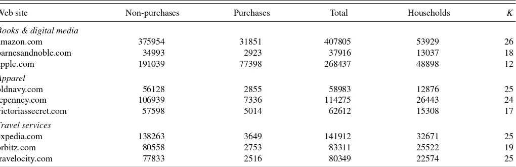
Web site Non-purchases Purchases Total Households K Books & digital media
amazon.com 375954 31851 407805 53929 26 barnesandnoble.com 34993 2923 37916 13037 18 apple.com 191039 77398 268437 48898 12
Apparel
oldnavy.com 56128 2855 58983 12876 25
jcpenney.com 106939 7336 114275 26443 24 victoriassecret.com 57598 5014 62612 15308 17
Travel services
expedia.com 138263 3649 141912 32671 25
orbitz.com 80558 2753 83311 25522 19
travelocity.com 77833 2516 80349 22574 25
capture the dependence structure between these four variables, which we show is more nuanced in our empirical work.
Instead, we construct the joint distribution via composition as
F(S, B, D, P)=F1(S, D|B, P)F2(B|P)F3(P), (2.1) from the component distributionsF1, F2, and F3. This has a number of advantages. First, with an appropriate choice of com-ponent distributions, nonlinearities, and other complexities in the dependence between the sales and Web site visit variables can be uncovered. We derive the purchase probability and ex-pected sales amount, conditional on the visit variables, to pro-vide insight into these relationships. Second, the degeneracy of
Sat 0 is easily accounted for by modelingF1differently when B=1 orB =0. Third, we identify parametric distributions for each component in Equation (2.1) that fit our Web site data well, distributions that have been used to model similar vari-ables previously. Furthermore, some of the components can be modeled semiparametrically, a property that will be exploited to handle retailers that make most sales at a small number of discrete price points. Fourth, estimation of the parameters of the distribution in Equation (2.1) is straightforward using maximum likelihood. Last, because Equation (2.1) is a fully specified joint distribution, it can be readily extended to account for market segmentation, as we show in Section4.
In building our model we first select an appropriate distribu-tion for the total number of page views per visit, denoted asF3. A popular model for page views is the negative binomial distribu-tion (NBD), which has been used previously by Danaher (2007) and Huang and Lin (2006). The distribution can be derived as a Gamma–Poisson mixture and is robust to observation-level heterogeneity. In our database, each observation corresponds to a visit to a retailer’s Web site, where at least one page is viewed, soP ≥1. To account for this we truncate the NBD by removing the zero case from the probability mass function.
The remaining two distributionsF1andF2in the decompo-sition of Equation (2.1) are both conditional on the number of page views. We account for this by making the parameters of the two distributions functions ofP. In particular, we partition
Pinto contiguous intervals ˜P1,P˜2, . . . ,P˜Kthat cover the range
ofP, and allow the parameters of F1 andF2 to differ in each partition, so they are step functions with respect toP. We select the partition cut points for each Web site so that there are ap-proximately an equal number of visits that result in a purchase within each partition. We select the number of partitions using five-fold cross-validation as discussed in Section 2.3. In our empirical work, we show that this greatly enhances the quality of fit, as well as substantially improving prediction accuracy. Conditional on the page view partition, we model the purchase indicator,F2(B|P ∈P˜k), with a Bernoulli distribution.
The bivariate distribution of sale amount and duration of visit, denoted asF1, differs depending on whether or not a purchase occurs during the visit. When there is no purchase (B=0), the bivariate distribution is degenerate atS=0, so thatF1(S= 0, D|B=0, P ∈P˜k)=F1D(D|B =0, P ∈P˜k). The
distribu-tionF1D(D|B =0, P ∈P˜k) is univariate and relates only to the
Web site duration, and is well-modeled as an inverse Gaussian. This distribution was identified as optimal using AIC and BIC from a list of alternative distributions that also included the
Gamma, Weibull, log-logistic, and log-normal. It has also been used previously to model duration over heterogeneous popula-tions (Hougaard1984; Johnson, Kotz, and Balakrishnan1994, p. 291), which is precisely the situation here.
However, when a purchase does occur, so that S >0, then F1 is a bivariate distribution which we model using a copula model, as now detailed. We label the two univariate distributions as F1S(S|B=1, P ∈P˜k) and F1D(D|B=1, P ∈P˜k), which
makes explicit the conditioning on purchase incidence and page views. We “couple” these together using a bivariate copula func-tionCwith dependence parameterθkthat varies over partition,
so that
1 is an inverse standard nor-mal distribution function and2is the distribution function of a bivariate normal distribution with zero mean, unit marginal vari-ances, and correlation−1< θ <1. The copula only accounts for any dependence between the two variables; with positive de-pendence whenθ >0, negative dependence whenθ <0,and independence when θ =0; see Song (2000) for a discussion of the Gaussian copula. Other bivariate copulasCcan also be employed easily here, with comprehensive lists given by Nelsen (2006), McNeil, Frey, and Embrechts (2005) and Trivedi and Zimmer (2005). The Gaussian copula has symmetric tail de-pendence (McNeil, Frey, and Embrechts 2005, pp. 208–222), which proves an unrealistic assumption in risk management applications. To investigate if this is also unrealistic here, we considered a copula constructed as a linear combination of a Clayton, Gumbel, and Gaussian copulas. The Clayton copula allows for lower tail dependence and the Gumbel for upper tail dependence. When estimated using maximum likelihood for the data from amazon.com, we found minor or no meaningful tail dependence for any page view partition, and therefore retain the Gaussian copula for its robustness and simplicity.
For the univariate distribution of visit duration we again em-ploy an inverse Gaussian, but for sales amount we emem-ploy a log-logistic distribution. These were identified as optimal, us-ing AIC and BIC, from alternatives that included the Gamma, inverse Gaussian, Weibull, log-logistic, and log-normal distri-butions. We note that the log-logistic has been used to model sales amount previously by Oyer (2000).
For apple.com, the 77,398 recorded sales occur at only 151 nonzero price points, with 87.33% of all purchases being for ex-actly$0.99, which corresponds to the sale of a single song from the iTunes store. The next most popular price point, representing 4.76% of total purchases is$9.99, and corresponds to the pur-chase of an album. Clearly, the sales amountSdoes not follow a log-logistic distribution, or any other well known parametric distribution. For this retailer, we therefore employ the empirical distribution function (EDF) forS in each page view partition, giving an estimated distribution function ˆF1S(s|B=1, P ∈P˜k)
for eachk. This is a nonparametric estimator for each ordinal-valued distribution, with values at all the unique observed price points. The ability to combine parametric copula functions with
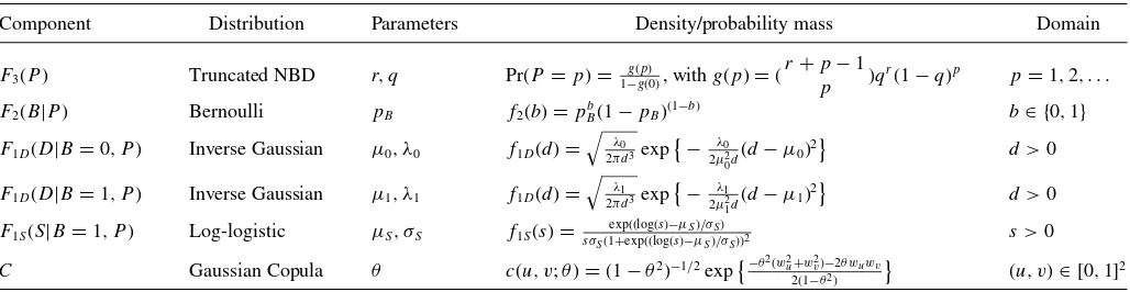
Table 3. Component distributions in the joint distribution of (S, B, D, P) in Section2. Apart from the truncated NBD, the parameters vary over theKpage view partitions. For the Gaussian copulawu=−1(u) andwv=−1(v), withbeing the standard normal distribution
function. Note that the log-logistic distribution is replaced by the empirical distribution function in the case of apple.com to account for highly discrete pricing
Component Distribution Parameters Density/probability mass Domain
F3(P) Truncated NBD r, q Pr(P =p)= 1−g(gp(0)) , withg(p)=(
one or more nonparametric marginal distributions is widely con-sidered a strength of the copula approach to constructing bivari-ate distributions (Shih and Louis1995).
Table 3lists the component distributions in the model, includ-ing their probability density or mass functions and unknown parameters. For the Web sites other than for apple.com, there are eight parameters for each page view partition and two for the modified NBD for the number of page views itself, resulting in 8K+2 parameters in total.
2.3 Estimation
When parametric distributions are used for the components in Equation (2.1), each component can be estimated using maxi-mum likelihood, and the resulting point estimates also maximize the joint likelihood. The parameters of the distributions ofF1 andF2are estimated separately for each partition, andF1 also for the two values ofB. WhenB=1, estimation of the bivariate copula model in Equation (2.2) is also straightforward using maximum likelihood, as outlined in Cherubini, Luciano, and Vecchiato (2004; pp. 154–156). The ease with which copula models can be estimated is one reason for their popularity.
In the case of discrete pricing, estimation of the bivariate distributionF1 differs becauseF1S(S|B=1, P ∈P˜k) is
mod-eled as a nonparametric discrete distribution using the EDF. The parameters of F1D(D|B =1, P ∈P˜k) are estimated
us-ing maximum likelihood, as is each copula parameterθk, but
conditional on the two estimated margins as follows. For each page view partition, given the EDF forSand estimated inverse Gaussian distribution for durationD, the likelihood can be cal-culated as follows. Let (si, di) be the ith observation of the
pair (S, D), uD,i =Fˆ1D(di|B=1, P ∈P˜k), bi =Fˆ1S(si|B=
1, P ∈P˜k) and ai =Fˆ1S(si−|B=1, P ∈P˜k) be the left-hand
limit of the step function ˆF1S atsi. Then, the mixed density of
(S, D) is obtained by differencing with respect to the discrete-valuedS, and differentiation with respect toD. The conditional likelihood for partitionkis
sian density, and the product is taken only over observations
iwhere sales are made (B=1) and with page views in par-titionk. This likelihood is easily maximized with respect to −1< θk <1 by grid search. This approach to estimating a
bi-variate copula model is widely called “inference for margins,” which Joe (2005) showed provides consistent estimates with only a very minor reduction in efficiency compared to full max-imum likelihood when the marginal distributions are known.
Last, we select the number of partitionsKfor each Web site using five-fold cross-validation (CV). For each foldj, the metric is the score CVj =i∈Foldjlog( ˆf(Si, Bi|Pi, Di)), where the summation is over the observations in foldj, and the mixed density is from the model fitted using the other four folds; the overall score is CV=5
j=1CVj. The mixed density is
computed asf(S, B|P , D)=f(S|B, P , D)f(B|P , D), where f(S|B, P , D) is derived from the copula model for F1, and f(B|P , D) is computed as in Equation (2.3). The last column ofTable 2gives the optimal number of partitions in the range 1–30 identified by this approach for all nine Web sites examined in our study.
2.4 Putting the Model to Use
Our primary aim is to understand the impact of the visit variables on both sales and purchase incidence. A simple, yet useful, summary measure is the overall (or “marginal”) level of pairwise dependence between all six pairs of variables. Spear-man’s rho is an appropriate measure of dependence even when the margins are far from Gaussian, and can be computed for the distribution in Equation (2.1) by first simulating many iter-ates from this distribution, and then computing the correlation coefficient of the ranked iterates. To simulate an iterate, first simulateP ∼F3, thenB ∼F2 and then (S, D)∼F1. For the latter, ifB=0 thenS=0 and onlyDneeds generating; while ifB =1 then the pair are generated from a bivariate Gaussian copula as outlined in Cherubini, Luciano, and Vecchiato (2004, p. 181). The pairwise dependence betweenSandD, conditional on a purchase made (B =1) and page views P, can also be computed for the bivariate Gaussian copula, with Spearman’s rhoρC
k =(6/π)arcsin(θk/2). We label this with a superscript
“C” to distinguish it from the marginal Spearman’s rho.
The impact of page views and duration can be assessed by evaluating the expected sales amount and probability of pur-chase, conditional on the visit variables as follows. The proba-bility of a purchase is
verse Gaussian densities computed at pointD, and Pr(B|P) is the Bernoulli purchase probability.
The expected salesE(S|D, P)= sf(s|D, P)dsis obtained via univariate numerical integration, except in the case of ap-ple.com where the discrete domain of sales is summed over in-stead. The density (or mass function for apple.com)f(s|D, P) can be derived analytically from the components as follows. First, note that
wheref1,f1D, andf1Sare the density functions of distributions
F1, F1D, andF1S, andc(u, v;θ)= ∂ 2C
∂u∂v is the copula density.
The copula density for a bivariate Gaussian copula is given in Table 3. For sales amount with a discrete distribution
f(s|B=1, D, P)=[ ˜C(b|F1D(D|B=1, P);θ)
−C˜(a|F1D(D|B =1, P);θ)], (2.4)
whereb=F1S(s|B=1, P) anda=F1S(s−|B =1, P) is the
left-hand limit ofF1Sats.
An advantage of computing the conditional expectation E(S|D, P) and probability Pr(B=1|D, P) from Equation (2.1), rather than modeling them explicitly, is that it captures the contemporaneous and nonlinear dependence between all four variables. We use the conditional expectation and purchase probability derived above in our empirical work in Section3. We also use them to make predictions in a validation study to further motivate our model, as discussed below.
2.5 Model Validation
We demonstrate that our model improves prediction of sales, conditional on both visit variables, compared to some alternative approaches. These include a na¨ıve forecast as a benchmark, linear modeling, a popular data-mining method, and a survival model from the marketing literature. We also show that forecasts constructed using both visit variables are more accurate than those that use only one.
We apply these approaches to the nine Web sites examined in detail in Section 3. The holdout sample size is nf =5000
for seven sites, and nf =10,000 for the two sites with the
largest number of observations, amazon.com and apple.com. The holdout sample is stratified with respect to sales amountS, so that it is more representative than a simple random sample, although the conclusions are the same in either case. We fit our model to the data for each Web site and compute the probability of a purchase ˆbi, and expected sales ˆsi, for each observationiin
the holdout sample using the expressions in Section2.4. These are used to predict purchase incidence and sales amount. We label our method “SM,” and compare it to alternative methods which construct forecasts as follows.
• Na¨ıve (N): The historical purchase incidence ( ˆbi =B¯), and
the average sales amount ˆsi =S¯.
• Linear model (LM): A probit model for purchase inci-dence, and a regression model for the logarithm of the sales amount of transactions, both with D andP as lin-ear covariates. The probability of a sale ˆbi is computed
from the probit model, and expected sales as ˆsi=E(S|B=
1, Di, Pi)×bˆi, whereE(S|B=1, Di, Pi) is the expected
sales for a transaction obtained from the regression model. • CART: We employ the popular “Classification and Re-gression Tree” data-mining method withDandPas input variables; once for purchase incidence, and a second time for the logarithm of sales amount of transactions. Fore-casts for sales amount for all visits are then computed by multiplication in the same manner as for the linear model. • Survival model(M06): This is an adaptation of the basic survival model proposed by Manchanda et al. (2006) for online purchase incidence. These authors employ a propor-tional hazard model with an advertising exposure measure as a covariate, a step function for the baseline hazard, and only observe purchases. In comparison, we employ page views as a covariate, an empirical distribution function for the baseline hazard (i.e. a Cox proportional hazards model), and employ both purchase and nonpurchase visits. • SMP: This is a trivariate variant of our model excluding
du-ration, so that forecasts are constructed conditioning only on page views.
• SMD: This is a trivariate variant of our model excluding page views, so that forecasts are constructed conditioning only on duration.
For each method, we compute the root mean square error (RMSE), both for predictions of purchase incidence and sales amount, except for M06 which only provides predictions of purchase incidence.Table 4summarizes the predictive accuracy of all methods over the holdout samples for all nine Web sites. The RMSE value is reported for SM, and percentage deviations from this value are reported for other methods. Positive deviations correspond to increases in RSME and therefore lower accuracy. If the squared errors are not significantly different using a matched-pairs test at the 95% confidence level, then the percentage difference figure is given in italics.
A number of conclusions can be drawn from the results. First, our proposed model (SM) provides forecasts that are more ac-curate than the na¨ıve benchmark,N, and the competing methods
Table 4. Predictive performance of the different methods for all nine Web sites in the validation study, including the mixture model in Section4
(MIX). The root mean square error (RMSE) of forecasts for purchase incidenceB, and also sales amountS, are reported for method SM (our proposed stochastic model). For the other methods, the percentage difference between the RMSE values for each method, and that for SM, is reported. Positive percentages correspond to an increase in RMSE compared to method SM, and therefore lower predictive accuracy. When these are not significantly different from zero, then the percentage figure is given in italics. A mixture model was not considered for the Web
site apple.com, so that no value is reported for this case
Purchase incidence Sales amount
Retailer SM N LM M06 CART SMP SMD MIX SM N LM CART SMP SMD MIX
Books & digital media
bn.com 0.245 8.8% 5.7% 7.0% 9.8% 0.4% 3.7% −0.9% 21.53 2.1% 2.1% 2.1% 0.8% 0.8% 1.9%
amazon.com 0.247 8.6% 5.7% 7.6% 2.9% 0.7% 4.6% −3.7% 26.29 2.8% 3.0% 2.7% 0.3% 1.4% −1.4% apple.com 0.440 3.0% 1.2% 8.9% 0.7% 1.3% 0.8% – 1.62 4.9% 3.5% 0.1% 6.6% 4.6% –
Travel Services
expedia.com 0.151 5.7% 3.7% 4.0% 11.2% 2.7% 0.5% 1.1% 111.87 3.1% 3.4% 7.5% 0.4% 1.4% 2.2% travelocity.com 0.165 5.8% 3.1% 2.7% 10.0% 1.1% 1.4% 0.8% 114.65 3.3% 5.8% 11.0% 0.9% 0.5% 4.7% orbitz.com 0.168 6.9% 4.8% 4.8% 7.8% 1.6% 1.9% 0.9% 97.53 4.1% 5.4% 6.5% 1.1% 1.3% 3.2%
Apparel
vic’ssecret.com 0.248 9.5% 2.5% 5.6% 9.6% 3.4% 2.0% −2.4% 37.60 8.4% 3.1% 7.9% 2.9% 1.6% −2.0%
oldnavy.com 0.196 9.0% 2.4% 4.5% 10.9% 1.5% 2.8% 1.3% 20.13 7.5% 3.1% 8.8% 1.2% 2.5% 4.2%
jcpenney.com 0.231 5.8% 2.3% 3.2% 7.9% 2.5% 0.6% −0.8% 38.83 3.2% 1.6% 8.1% 1.3% 0.3% 1.4%
LM, M06, and CART. The differences are significant for both forecasts of purchase incidence and sales amount, except for CART forecasts for apple.com. Second, it is clear that the du-ration of a visit and the number of page views are useful in forecasting sales incidence and amount, withNdominated, par-ticularly for retailers of apparel. Third, including bothDandP
as predictors improves forecast accuracy over-and-above using either separately. Fourth,Table 4also includes validation results for a mixture model, but we discuss these in Section4where it is introduced. Last, we note that small improvements in forecast accuracy for each visit have the potential to make a substantial impact because of the very large number of visits. For example, our panel of approximately 100,000 users made over 407,000 visits to amazon.com in 2007, so the total number of visits by U.S. Internet-enabled households to this Web site alone would number in the hundreds of millions during that year.
3. EMPIRICAL ANALYSIS
We now demonstrate the usefulness of our stochastic model for investigating the relationship between the Web site visit vari-ables, purchase incidence, and sales for major online retailers in three product categories: books and digital media, travel ser-vices, and apparel. We showcase apple.com separately, given its unique online retail product assortment and its highly discrete pricing structure.
3.1 Books and Digital Media
The first Web site we examine is amazon.com, which was the world’s largest online retailer by total sales in 2007. Amazon.com sells products in a wide variety of classes, but has a particular focus on books (47% of sales) and digital media products, such as DVDs and CDs of movies and music (28% of sales). There are 407,805 visits by comScore panelists to
amazon.com in our data, with 31,851 (7.81%) of these visits re-sulting in a purchase.Table 5contains the page view partitions, and the number of observations in each page view range.
Table 6reports the parameter estimates and 95% confidence intervals for the component distributions in Equation (2.1), and it can be seen that all the parameters vary substantially over the page view ranges. From the estimates for the distribution F2, the probability of a purchase being made when the number of page views is between 1 and 7 is low at Pr(B =1|1≤P ≤ 10)=0.6%. As one would expect, this increases monotonically with the number of page views, so that for visits with between 76 and 99 page views the probability of a purchase rises to Pr(B=1|76≤P ≤99)=30.9%. For each bivariate Gaussian copula, we also compute Spearman’s rho for the dependence between sale amount and visit duration, assuming a purchase occurs. This is also reported inTable 6, and is positive for all but one page view partition, with the largest value being 0.106. Thus, it might initially appear that dependence between the duration of a visit and the sale amount is quite low. However, Table 7reports the matrix of pairwise marginal Spearman cor-relations, and that between duration and sale amount is ˆρS,D =
0.259. To illustrate the usefulness of our model,Table 7also contains the marginal Pearson sample correlations, which differ from the Spearman correlations because they do not take into ac-count the highly non-Gaussian distribution of the variables. The Pearson correlations understate substantially the relationship be-tween both visit variables (DandP) and the sales amount (S).
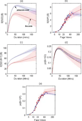
We also compute expected sales, conditional on both duration, and page views.Figure 1plots the results as a three-dimensional surface “sliced” at the mid-point of each page view partition. As the number of page views increase there is a corresponding increase in the expected sale amount. However, the same is not true for duration, with there being a visit duration that results in a maximum level of expected sales for each page view level. The relationship of the two visit variables with expected sales
Table 5. Optimal page view partitions for the two book retailers, presented as two adjacent partitions per row. The sample sizes in the paired partitions are reported, broken down by observations where no sale was made, and those visits where one or more items were purchased
amazon.com (K=26) bn.com (K=18)
k P˜k No sale Purchases P˜k No sale Purchases
1 & 2 1–7, 7–9 244266 2523 1–10, 11–13 26261 394 3 & 4 10–11, 12–12 33360 2732 14–15, 16–16 1879 283 5 & 6 13–13, 14–14 15163 2105 17–18, 19–20 1699 370 7 & 8 15–16, 17–17 17009 2964 21–22, 23–23 935 254 9 & 10 18–18, 19–20 12481 2640 24–26, 27–29 1260 373 11 & 12 21–21, 22–23 9168 2348 30–32, 33–35 795 281 13 & 14 24–24, 25–26 7296 2045 36–40, 41–46 848 326 15 & 16 27–28, 29–30 7126 2316 47–54, 55–66 681 319 17 & 18 31–33, 34–35 6368 2395 67–92, 93–500 635 323 19 & 20 36–39, 40–43 6924 2747
21 & 22 44–47, 48–54 5811 2295 23 & 24 55–62, 63–75 5313 2353 25 & 26 76–99, 100–500 5651 2388
Total 375954 31851 34993 2923
cannot be represented in an additive fashion and is instead a bivariate nonlinear iteration.
Figure 1shows that the link between the two visit variables and expected sales is very different for each variable. We ex-amine this further by computing expected sales, marginalizing, respectively, over page views and duration. These expectations can be computed in a closed form, as detailed in the Appendix. Starting with the expected sale amount and duration relationship
(marginalizing over page views), denotedE[S|D],Figure 2(a) shows that expected sales peak at $14.50 for visits of duration of 59 minutes. In contrast, a plot of expected sales against page views (E[S|P]) inFigure 2(b) shows that sales simply increase monotonically as page views increase.
Figure 2(c) graphs the expected sales conditional on duration when a purchase is made (i.e.,E[S|D, B=1]), showing that expected sales increase monotonically as a function of duration
Table 6. Estimates of the parameters of the stochastic model for amazon.com, with 95% confidence intervals given below in parentheses. To save space, only estimates for the 13 odd numbered partitions are given
Page views Copula dependence F1S(S|B=1, P) F1D(D|B=1, P) F1D(D|B=0, P) F2(B|P)
(P) θˆ ρˆC μˆ
S σˆS μˆ1 λˆ1 μˆ0 λˆ0 pˆB
1≤P ≤7 0.085 0.081 3.24 0.481 4.76 5.21 4.41 2.98 0.006
(0.018,0.15) (3.19,3.28) (0.46,0.504) (4.51,5.00) (4.81,5.61) (4.39,4.43) (2.97,3.0) (0.006,0.007)
10≤P ≤11 0.064 0.061 3.23 0.477 8.54 13.6 10.1 9.38 0.067
(0.013,0.115) (3.19,3.27) (0.459,0.496) (8.22,8.86) (12.7,14.5) (10.0,10.3) (9.2,9.5) (0.064,0.07)
13≤P ≤13 −0.001 −0.001 3.28 0.469 10.2 21.1 12.3 12.9 0.118
(−0.062,0.061) (3.233.33) (0.446,0.493) (9.80,10.7) (19.3,22.9) (12.0,12.5) (12.5,13.3) (0.111,0.124)
15≤P ≤16 0.053 0.051 3.31 0.487 12.3 27.9 14.5 16.8 0.143
(0.01,0.096) (3.27,3.35) (0.469,0.505) (11.9,12.7) (26.2,29.7) (14.3,14.7) (16.3,17.2) (0.138,0.149)
18≤P ≤18 0.078 0.075 3.39 0.496 15.5 35.1 16.3 20.1 0.164
(0.015,0.141) (3.34,3.45) (0.47,0.523) (14.8,16.1) (31.9,38.3) (15.9,16.7) (19.2,20.9) (0.155,0.174)
21≤P ≤21 0.111 0.106 3.42 0.481 17.5 46.6 18.7 25.3 0.184
(0.043,0.178) (3.36,3.48) (0.454,0.511) (16.7,18.2) (41.9,51.2) (18.2,19.3) (24.1,26.4) (0.173,0.196)
24≤P ≤24 0.065 0.062 3.48 0.498 19.4 55.2 21.1 31.6 0.209
(−0.004,0.134) (3.42,3.54) (0.468,0.53) (18.6,20.3) (49.4,61.0) (20.4,21.7) (29.9,33.3) (0.195,0.223)
27≤P ≤28 0.054 0.051 3.55 0.483 22.9 69.8 23.0 37.4 0.239
(−0.002,0.109) (3.50,3.60) (0.461,0.507) (22.2,23.7) (64.2,75.4) (22.5,23.6) (35.7,39.1) (0.227,0.251)
31≤P ≤33 0.043 0.041 3.56 0.503 26.0 79.9 26.0 42.5 0.268
(−0.007,0.092) (3.52,3.60) (0.482,0.524) (25.3,26.8) (74.2,85.7) (25.4,26.6) (40.7,44.4) (0.256,0.279)
36≤P ≤39 0.013 0.013 3.60 0.519 28.8 104.7 29.5 56.4 0.281
(−0.036,0.062) (3.55,3.64) (0.498,0.542) (28.0,29.5) (97.2,112.2) (28.8,30.2) (54.0,59.0) (0.269,0.293)
44≤P ≤47 0.071 0.068 3.62 0.544 35.5 119.7 34.4 65.5 0.273
(0.011,0.131) (3.56,3.68) (0.516,0.574) (34.2,36.7) (108.9,130.5) (33.4,35.3) (61.9,69.1) (0.258,0.288)
55≤P ≤62 0.049 0.047 3.71 0.559 43.8 178.0 42.7 88.0 0.297
(−0.007,0.106) (3.65,3.77) (0.532,0.587) (42.5,45.1) (163.3,192.7) (41.5,43.8) (83.3,92.7) (0.283,0.312)
76≤P ≤99 0.079 0.075 3.79 0.580 59.7 224.7 55.0 143.0 0.309
(0.023,0.134) (3.73,3.85) (0.553,0.608) (58.0,61.5) (206.5,242.7) (53.7,56.3) (135.3,150.7) (0.294,0.323)
Parameters of the NBDF3: ˆr=0.7660 (±4.27×10⁻⁶); ˆq=0.0600 (±2.97×10⁻⁷); E(P)=13.56; Std. Dev.(P)=15.033
Table 7. Marginal pairwise Spearman dependence measures from the fitted model for amazon.com, and the Pearson sample correlations. The high Spearman dependence betweenSandBis due to the very strong zero-inflation of the sales data, which is commonplace in
online retail
among just those who eventually make a purchase. Clearly, pur-chase incidence has a role to play.Figure 2(d) and (e) give the purchase probability conditional on, respectively, duration and page views. These are computed by marginalizing out the other variable as outlined in the Appendix.Figure 2(d) reveals that, for amazon.com, purchase incidence as a function of duration (Pr(B =1|D)) increases then declines, whileFigure 2(e) shows that purchase incidence always increases as a function of page views. Hence, the reason for the differences betweenFigure 2(a) and (b) is that purchase incidence rises then declines as dura-tion increases, but purchase incidence always increases as more pages are viewed. A likely reason for the effect observed in Figure 2(d) is that there is one or more segments of buyers who are goal-directed and therefore time-efficient in their purchase behavior. By contrast, members of other segments are simply browsing a Web site and are eventually tempted to purchase af-ter a lengthy visit (see also Bucklin and Sismeiro2003; Danaher and Mullarkey2003). Hence,Figure 2(d) plots likely due to a
0 50
Figure 1. Expected sale amount at amazon.com as a function of duration of visit and number of page views (on the logarithmic scale) resulting from the parametric model. Note that the impact of duration and page views on expected sales is not additive in form.
mixing of these broad segments. In Section 4, we show how our model can be extended to incorporate latent segmentation household-level heterogeneity.
Barnes and Noble are the second largest online book retailer in the United States, so we also look at their Web site bn.com for comparison. The site offers a product range based primarily around books, in contrast to Amazon’s broader offering. In 2007, Barnes and Noble had approximately 9% of the traffic and 6% of the total sales of the much larger retailer Amazon. Nevertheless, Table 5shows that the partitions for the page view deciles for these two retailers are broadly similar.
Figure 2also plots expected sale amount and probability of purchase for visits to bn.com, conditional on the Web site visit variables for the fitted model. In comparison to amazon.com, expected sale amount peaks for slightly shorter visits of duration 52 min, but at a much lower value of just over $10.08. Clearly, amazon.com proves to be more successful at converting each individual visit to a higher sales amount. Moreover, if a purchase does occur, Figure 2(c) shows that the expected sale amount does not increase as quickly with duration as for amazon.com. However, there appears to be little difference in the underlying purchase rates for these two Web sites. Figure 2(d) and (e) reveal that the purchase probability conditional on, respectively, duration and page views are similar for both Web sites. Hence, the difference in expected sale amount appears to result from higher basket totals at amazon.com. Interestingly, visits with very similar durations of 42.4 and 41.2 min have the maximum purchase probability for amazon.com (0.23) and bn.com (0.23), respectively.
3.2 Apparel and Travel Services
Table 1 shows that the retailers jcpenny.com, victoriasse-cret.com, and oldnavy.com are the fifth, sixth and seventh largest retailers as measured by total number of purchases. All three are major apparel retailers, although jcpenny.com has the most di-versified product lineup, victoriassecret.com is a niche retailer, and oldnavy.com sells family fashion and accessories. In addi-tion,Table 1shows that the sites expedia.com, orbitz.com, and travelocity.com are the third, fifth, and seventh largest retailers as ranked by total value of sales. They all provide travel services and have a product portfolio that is more homogenous than the three apparel retailers. We estimate our stochastic model for each of these six sites and present some of the key relationships between sales and visits inFigure 3.
Figures 3(a) and (c) show that victoriassecret.com and jcpenny.com both derive higher sales from visits than old-navy.com; presumably due to their differing product lineups. More interestingly, it appears that victoriassecret.com is par-ticularly successful in translating visits with longer durations into higher sale amounts when a purchase is made. Moreover, all three apparel retailers appear to convert higher duration vis-its into higher sales more effectively than either the two book retailers or three travel service providers.
Figure 3(b) shows that the three travel service providers have differing degrees of success at converting visits of longer duration into sales amounts. Travelocity.com is most successful, with the highest expected sale amount of $141.80 for visits
Figure 2. Expected sale amount and purchase probabilities per visit at amazon.com and bn.com for the stochastic model. Panel (a) plots expected sale amount conditional on visit duration; panel (b) plots expected sale amount conditional on the number of page views; panel (c) plots expected sale amount conditional on visit duration for situations where a purchase is made (i.e.,B=1); panel (d) is the purchase probability against the visit duration; panel (e) is the purchase probability against the number of page views. Ninety percent confidence intervals, calculated using the bootstrap, are plotted as light shaded intervals in each panel and for both Web sites.
of duration 112 min. The differences between the three sites appear driven entirely by differing abilities to convert longer duration visits into purchase events. Once the expected sale amount is computed, conditional on a purchase being made, there is minimal difference between the three travel service providers as depicted in Figure 3(d), which likely reflects the similarity of the products offered at these travel Web sites.
Figure 3(e) and (f) depict the probability of a sale being made against the number of page views for the six Web sites. Gen-erally, higher page views correspond to a higher probability of purchase. Interestingly, the sites that are least successful at con-verting longer duration visits into sales are not necessarily poor at converting more page views into more purchases. For exam-ple, oldnavy.com has the highest purchase probability among all retailers, as the number of page views increases.
0 50 100 150 0
20 40 60 80
Duration (mins)
E[S|D] ($)
(a)
0 50 100 150
0 50 100
Duration (mins)
E[S|D] ($)
(b)
0 50 100 150
0 50 100 150 200
Duration (mins)
E[S|D, B=1] ($)
(c)
0 50 100 150
0 200 400 600 800
Duration (mins)
E[S|D, B=1] ($)
(d)
10 20 60 200 0
0.1 0.2 0.3 0.4
Page Views
pr(B=1|P)
(e)
10 20 60 200 0
0.05 0.1 0.15 0.2 0.25
Page Views
pr(B=1|P)
(f)
victoriassecret.comjcpenney.com
oldnavy.com
travelocity.com
orbitz.com
expedia.com
Figure 3. Relationships between sales and visitation variables for online apparel retailers in panels (a), (c), and (e), and online travel service providers in panels (b), (d), and (f). Panels (a) and (b) present the expected spend conditional on duration of visitE(S|D). Panels (c) and (d) present the expected spend conditional on duration and that a purchase is made,E(S|B=1, D). Panels (e) and (f) depict purchase probability conditional on the number of page views, Pr(B=1|P).
3.3 Research Online and Buy Online Later
A final observation that applies just to the apparel retailers concernsFigure 3(c). A subtle feature of this plot is a small dip in sales between 5 and 10 min. This is due to some short-duration visits (less than 10 min) where the expected sales are relatively high. We conjecture that this is due to recent
prior visits to the Web site that are strictly browsing, without a sale being made. During this time a shopper likely peruses the merchandise, possibly checking out competing Web sites. Eventually when the decision to purchase is made, the transac-tion time is relatively quick, because product research has been completed prior to the actual purchase visit. The likelihood of such behavior is very plausible because online research prior to
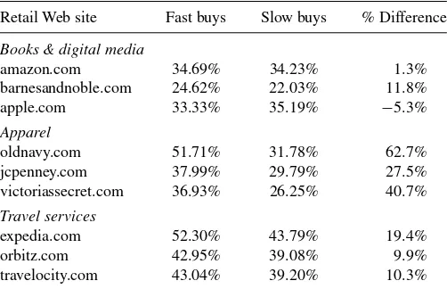
Table 8. Proportion of households who visit a site 48 hr prior to ultimately making a purchase. The values are broken down into two
groups: those where the purchase is made quickly within duration
D≤10 min, and those made slowly inD >10 min. The final column reports the percentage difference between these two proportions Retail Web site Fast buys Slow buys % Difference
Books & digital media
bricks-and-mortar purchase is commonplace (Krillion 2008; Mendelsohn, Johnson, and Meyer2006). All we are suggest-ing here is the eventual purchase is made online rather than in-store.
We test this conjecture by dividing purchase visits into those that are fast (≤10 min) and slow (>10 min), and then calculate the proportion of households in these two groups that have visited the same Web site within 48 hr prior to the eventual purchase visit, but have not purchased anything during those prior visits.Table 8reports these proportions. Fast purchasers of apparel products research online before making the purchase much more often than slow purchasers (between 27.5% more often for jcpenney.com and 62.7% more often for oldnavy.com), consistent with our conjecture. This behavior is replicated by purchasers of travel services, but to a lesser extent. However, there is very little difference between the online product research undertaken by fast and slow purchasers of books or digital media products, where the purchase risk is lower.
3.4 Discrete Sales Categories for Apple.com
Apple.com has a high rate of conversion of visits into pur-chases at 29.1% in 2007. Moreover, the estimated relationship between Web site visit and sales variables is very different to that of the other retailers in our study.Figure 4shows the prob-ability of purchase against duration inFigure 4(a) and number of page views inFigure 4(b). Apple.com visitors have much fewer page views on average than other online retailers, but these convert much more rapidly into higher purchase proba-bilities compared with retailers in our study. The expected sale amount is low because sales are predominantly for a single song. For visits where a purchase is made, Figures4(c) and (d) plot the expected sale amount against duration and page views, re-spectively. The expected sale amount peaks strongly at visits of duration 4 min. Compare this to the relationship for retail-ers of books, apparel, and travel services (Figures2(c), 3(c), and (d)), where purchasing visits have a higher expected sale amount as duration increases. For visits with a small number of
page views, the expected sale amount at apple.com is close to $0.99. However, this increases markedly for visits with 10 or more page views.
We also compute the Spearman’s correlations between the variables for the fitted stochastic model. There is a lower de-pendence between the visit and sales variables when compared with amazon.com in Table 7. This is particularly true for the purchase indicator, with ˆρB,D=0.223 and ˆρB,P =0.183. This
suggests that visitors to apple.com are more goal-directed than those at amazon.com, as might be anticipated for a Web site that is tailored primarily toward transactions rather than browsing.
4. LATENT SEGMENTATION
4.1 Bayesian Model
While both the NBD and inverse Gaussian are popular model choices for data that arise from heterogeneous populations, it is likely the data exhibit further heterogeneity. For example, Moe and Fader (2004) proposed a taxonomy of four groups of on-line shoppers, based on visit behavior and purchase incidence. Therefore, to further account for household-level consumer het-erogeneity we employ a finite mixture model with latent seg-mentation. This approach is well established in marketing (Ka-makura and Russell1989; Allenby and Rossi1998), although usually using a mixture of normals, whereas we consider a mix-ture of the quad-variate stochastic models in Equation (2.1).
Consider a mixture withMlatent segments, and probabilityπl
that a household is a member of segmentl, then the distribution of the visit and sales variables is
F(S, B, D, P)=
where segments are denoted with a superscript.
Bayesian estimation of mixture models is popular, with pos-terior inference computed using Markov chain Monte Carlo (MCMC) methods; for example, see Diebolt and Robert (1994). This includes the ability to profile the segments, which can be difficult using other likelihood-based methods (Wedel and DeSarbo 2002). Latent multinomial variables are introduced to specify segment membership for each household h, where Lh=lif householdhis a member of segmentl. We denote the
set of latent variables for allHhouseholds asL= {L1, . . . , LH}.
Conditional on L, the likelihood of the mixture model is sim-plified with respect to the parameters of segment Fl. MCMC
samplers that generate the latent variables explicitly, and the pa-rameters conditional upon these, are popular; for example, see Diebolt and Robert (1994) and Lenk and DeSarbo (2000). In the supplementary material, we outline such a sampling scheme to generateJiterates from the posterior distribution of the mix-ture model parameters, augmented with the household latent variables.
In our Bayesian analysis, we adopt a Dirichlet prior for π =(π1, . . . , πM)∼Dirichlet(α), which is a common choice
0 50 100 150 0
0.1 0.2 0.3 0.4 0.5 0.6
Duration (Mins)
pr(B=1|D)
(a)
5 10 20 60 200 0
0.1 0.2 0.3 0.4 0.5
Page Views
pr(B=1|P)
(b)
0 50 100 150
0 0.5 1 1.5 2 2.5
Duration (Mins)
E[S|D,B=1] ($)
(c)
10 20 60 200 0
0.5 1 1.5 2 2.5
Page Views
E[S|P,B=1] ($)
(d)
Figure 4. Estimated relationships for apple.com. Panels (a) and (b) plot the purchase probability against visit duration and the number of page views. Panels (c) and (d) plot the expected spend against duration and number of page views for visits which result in a purchase.
because it has the Bayesian property of being conjugate to the multinomial. To make the mixture model more flexible, we makeαa hyperparameter with a uniform hyperprior on [0,2]M,
which ensures the prior onπis flat at the prior expected value of E(α)=1. The priors on the parameters of the component dis-tributionsF1l, F2l, F3l are the same across segments and proper, which is important to facilitate model selection, but noninfor-mative, so that the posterior distribution of the parameters is dominated by the likelihood. We select the number of seg-ments using a deviance information criterion (DIC), suggested by Celeux et al. (2006), which is more appropriate for model choice in mixture models than that introduced by Spiegelhalter et al. (2002). Adopting the notation of Fr¨uhwirth-Schnatter and Pyne (2010), this is defined for each value ofMas
DIC4a(M)= −4E[logL(;y)|y]+2 logL( ˆ;y)
+2E[EN()|y].
In the above,ydenotes the data,is the parameters of allM
segments, ˆis the posterior mode,Lis the likelihood, EN is the entropy, and the expectations are with respect to the posterior distribution. This criterion is more robust to label-switching; see
Lenk and DeSarbo (2000) and Stephens (2000) for discussions of this problem. The likelihoodLis from Equation (4.1), and the criterion can be computed efficiently using the output of the sampling scheme as discussed in Fr¨uhwirth-Schnatter and Pyne (2010, Sec. 3.3). We compute DIC4a(M) forM=1,2,3,4, and
selectM that maximizes its value. We found that for all Web sitesM=4 was the optimal value, except for oldnavy.com, which hadM=3 segments.
4.2 Predictions
Parameter estimates and other inference can be readily com-puted using the output from the sampling scheme. We es-timate the mixture model using the calibration data y, and then forecast purchase incidence and sale amount using the Bayesian predictive mass and expectation Pr(Bi =1|Di, Pi, y)
andE(Si|Di, Pi, y) for each visitiin the holdout sample of the
validation study. These differ depending on whether, or not, the householdhassociated with visit ialso had visits recorded in the calibration data. Nevertheless, they can be computed using the MCMC output in both cases, as outlined in the supple-mentary materials.Table 4includes the performance of these
forecasts in the MIX column. For amazon.com and victoriasse-cret.com, there is a significant increase in forecast accuracy. For the remaining sites forecasts are either not meaningfully im-proved, or slightly less accurate for sales amounts at the three travel sites.
4.3 Segmentation for Oldnavy.com
Also of interest are the profiles of the market segments. In Bayesian estimation, these are computed with the parameters and latent variables integrated out with respect to the posterior distribution, rather than conditional on their point estimates. For example, ifl denotes the parameters of thelth segment, then the mean of thelth fitted segment is
E(S, B, D, P|Lh=l, y)
=
E(S, B, D, P|Lh=l, l)f(l|y)dl
≈ 1 J
J
j=1
(S, B, D, P)[j].
Here, each iterate (S, B, D, P)[j] ∼f(S, B, D, P|L
h=
l, l,[j]) is generated from segment l with parameter values l,[j]∼f(l|y) obtained at sweepj of the MCMC sampling
scheme. Estimates of other moments or distributional sum-maries for each segment can also be computed in a similar fashion.
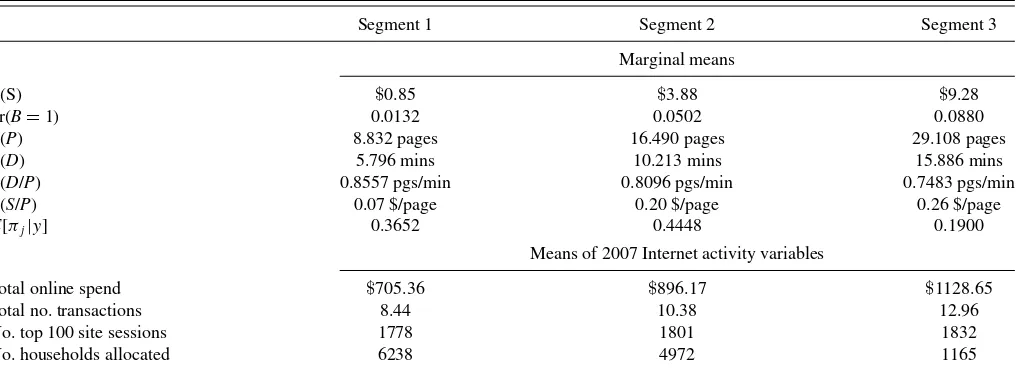
To illustrate,Table 9provides profiles for each of the three segments of oldnavy.com obtained using the calibration data. The top portion of the table reports the expectations of the four variables, and also the two ratiosP /DandS/P. The first ratio is a measure of how fast a visitor progresses through the site (i.e., search velocity), while the second ratio is a measure of a visitor’s expected spend in response to page exposure. Households in seg-ment 1 have low purchase incidence, low expected spend, and progress through the pages with the highest search velocity. In comparison, households in segment 3 have the highest purchase incidence, highest expected spend, and highest expected spend
per page. Moe (2003) and Moe and Fader (2004) characterize online shoppers into four groups:directed buyers, deliberation visitors, hedonic browsers,andknowledge-building visitors. For our oldnavy.com segmentation, Segment 1 has characteristics consistent with those of knowledge-building behavior, while households in Segment 3 exhibit goal-directed behavior that is more consistent with directed buyers and deliberation visi-tors. Segment 2 households have characteristics consistent with hedonic browsers.
The posterior probability that a specific household h is in segmentlis
Pr(Lh=l|y)=
Pr(Lh=l|π, , y)f(π, |y)d(π, )
≈ 1 J
J
j=1
Pr(Lh=l|π[j], [j], y)=ωˆhl. (4.2)
Here,{π[j], [j]}J
j=1 are the Monte Carlo iterates output from the MCMC scheme, and the supplementary material shows how to compute the conditional probability in Equation (4.2). The estimates ˆωlhdiffer for each household in the sample and should not be confused with an estimate of the probabilityπlin
Equa-tion (4.1), which is not household specific.
To see if the behavior of households in each segment extends beyond their activity at oldnavy.com, we also construct three general Internet activity variables for each household using the comScore transaction and session data. These are the total online spend, total number of online transactions, and total number of sessions at the top 100 Web sites across the entire year of 2007. Using the oldnavy.com data, for each householdhwe also com-pute the posterior probability of membership of each segment,
ˆ
ωjh, and allocate each observation to the segment with the high-est probability. The bottom row ofTable 9reports the number of households that are allocated to each segment, and the middle portion reports the sample means of the three general Inter-net activity variables. These show that the consumer behavior identified in our latent segmentation using the oldnavy.com data extends into similar general Internet activity at a household level.
Table 9. Profile of the segments in the fitted three segment mixture model for oldnavy.com. Top section: expected values of sales, purchase incidence, page views and duration, as well as the search velocity and sales per page viewed. Bottom section: means of the three household Internet activity variables for households allocated to each segment. Bottom Row: number of households in the calibration dataset allocated to
each segment using the mode of the household specific posterior probabilities
Segment 1 Segment 2 Segment 3 Marginal means
E(S) $0.85 $3.88 $9.28
Pr(B=1) 0.0132 0.0502 0.0880
E(P) 8.832 pages 16.490 pages 29.108 pages
E(D) 5.796 mins 10.213 mins 15.886 mins
E(D/P) 0.8557 pgs/min 0.8096 pgs/min 0.7483 pgs/min
E(S/P) 0.07 $/page 0.20 $/page 0.26 $/page
E[πj|y] 0.3652 0.4448 0.1900
Means of 2007 Internet activity variables
Total online spend $705.36 $896.17 $1128.65 Total no. transactions 8.44 10.38 12.96 No. top 100 site sessions 1778 1801 1832 No. households allocated 6238 4972 1165
5. CONCLUSION
In this research, we develop a stochastic model for Web site visit duration, page views, purchase incidence, and sales amount. Previous work has modeled the bivariate distributions of visit duration and purchase incidence (Lin et al.2010; Moe and Fader 2004; Montgomery et al.2004; Van den Poel and Buckinx2005), and visit duration and sales (Danaher and Smith 2011). However, ours is the first study to simultaneously handle all four of these key elements of online browsing and purchasing. From a managerial perspective, we show that the two stick-iness measures are important indicators of whether a sale will occur, and for the amount of the sale. This is consistent with an earlier empirical result by Montgomery et al. (2004), who were able to predict eventual purchase incidence with 40% accuracy using information from just the first six pages of a Web site visit. Interestingly, for books, digital media, and travel service Web sites there is a value of duration that maximizes expected sales, while expected sales generally increases monotonically with page views. Managers will also be interested to learn that while much attention has been devoted to research online, buy offline (e.g., Thackston2009), there is a parallel phenomenon of research online prior to purchasing (also) online. Such situa-tions are flagged by prior visits to a Web site, but the eventual purchase is comparatively quick in a subsequent visit. There-fore, online retailers should not necessarily be discouraged by the high proportion of nonsale visits (Moe and Fader 2004; Venkatesh and Agarwal2006). We found prior online research to be especially prevalent for apparel and travel products, no doubt because such categories entail more involved purchases, and the monetary amounts are higher, than for books, DVDs, and songs. We find that although Web sites within the same product category have different expected sales as a function of duration and page views, the relationship of these two visit variables with purchase incidence is similar. Therefore, it seems most likely that the difference in sales amounts is due to the product offer-ings. Our latent class segmentation for oldnavy.com identified three distinct market segments. The smallest segment consists of more engaged customers who exhibit greater goal-directed be-havior. Members of the largest segment exhibit browsing behav-ior, while those of the remaining segment are very low spending customers. Such segmentation is consistent with the classifica-tion discussed by Moe and Fader (2004), while profiling of the wider online activities of these households suggests that this behavior extends beyond their visits to oldnavy.com.
On the methodological front, we propose a quad-variate dis-tribution for the Web site visit and sales variables that is con-structed by composition from carefully selected components that fit well empirically. The framework has a number of prac-tical advantages. First, estimation is fast, so that the approach is practical given the very large size of the data that arise in studies of online retail behavior. Second, expectations of the sales variables, conditional on either visit variable separately, or both together, can be computed from the stochastic model without reverting to bivariate and trivariate numerical integra-tion. Third, computing these expectations from the quad-variate distribution, rather than modeling them directly in a regression style framework, accounts for the simultaneous determination of all four variables. Fourth, the model can extended to a finite mixture of the quad-variate distributions, so that consumer
het-erogeneity can be accounted for at the household level. Last, we adapt the model to cope with the discrete pricing used by retail-ers such as apple.com. To achieve this we exploit the flexibility of the bivariate copula component to model a combination of continuous and discrete marginals; something that would other-wise be difficult.
Our validation exercise shows that the proposed model out-performs a number of alternative approaches for the Web sites examined. This indicates that the nonlinear dependence between the variables is better captured by the model, and that the two Web site stickiness measures provide valuable information when predicting purchase incidence and sales. Importantly, our model is parametric and easy to extend into a variety of directions. Fu-ture work could include adding another layer to the model to incorporate Web site-level covariates, as used by Bucklin and Sismeiro (2003) and Danaher et al. (2006). This is straightfor-ward by making the parameters of the component distributions functions of the covariates, with estimation undertaken using maximum likelihood in the same manner as outlined. By us-ing time-based covariates, this also allows for the modelus-ing of dynamic behavior similar to that examined by Moe and Fader (2004). In addition, following Manchanda et al. (2006), a pos-sible further extension is a hierarchical model that incorporates household-level heterogeneity. This would provide an alterna-tive to latent class segmentation.
APPENDIX: SALES SUMMARIES
In this Appendix, we show how to use the stochastic model in Section
2.2to compute several summary measures of sales. These include both the probability of a purchase and the expected spend, both conditional upon only one visit variable and marginalized over the second. Page views can be marginalized over as follows:
Pr(B=1|D)=
Because the page view variable is partitioned intoK ranges in our stochastic model, the summations inPcan be replaced with summations over theKpartitions, so that
Pr(B=1|D)
summation over the mass function, and all other components in the expression above are known from the model definition, so that it can be computed analytically. Derivation of the expected spend con-ditional on duration only is similar. We first note that E(S|D)=
B=0,1
P=1,2,...E(S|D, P , B)Pr(P , B|D), but becauseS=0 when
B=0, this expression simplifies to
E(S|D)=
P=1,2,...
E(S|D, P , B=1)Pr(P , B=1|D).
The rest of the derivation follows the same expansion of Pr(P , B=
1|D) as above, and the substitution of the summations inPwith those