Full Terms & Conditions of access and use can be found at
http://www.tandfonline.com/action/journalInformation?journalCode=ubes20
Download by: [Universitas Maritim Raja Ali Haji] Date: 12 January 2016, At: 23:52
Journal of Business & Economic Statistics
ISSN: 0735-0015 (Print) 1537-2707 (Online) Journal homepage: http://www.tandfonline.com/loi/ubes20
A Failure in the Measurement of Inflation
Mick Silver & Saeed Heravi
To cite this article: Mick Silver & Saeed Heravi (2005) A Failure in the Measurement of Inflation, Journal of Business & Economic Statistics, 23:3, 269-281, DOI: 10.1198/073500104000000343
To link to this article: http://dx.doi.org/10.1198/073500104000000343
Published online: 01 Jan 2012.
Submit your article to this journal
Article views: 51
View related articles
A Failure in the Measurement of Inflation:
Results From a Hedonic and Matched
Experiment Using Scanner Data
Mick S
ILVERStatistics Department, International Monetary Fund, Washington, DC 20431 (msilver@imf.org)
Saeed H
ERAVICardiff Business School, Cardiff University, Cardiff CF10 3EU, U.K. (heravis@cf.ac.uk)
Statistical offices use the matched-model method to compile consumer price indexes to measure infla-tion. In markets where models turn over rapidly, the matched sample may, by the end of a year, be quite unrepresentative of what is and what was bought. An analytical model is derived to show how bias in a matched-model index arises and extended to shed further light on the influential Aizcorbe, Corrado, and Doms methodology. The empirical work on the bias is undertaken using monthly scanner data for five products: washing machines, dishwashers, television sets, cameras, and vacuum cleaners. Different strate-gies are explored that might ameliorate the bias, including using replacement models for old unmatched models, with hedonic adjustments to prices, more frequent sample rotation, and hedonic indices.
KEY WORDS: Consumer price index; Hedonic index; Hedonic regression; Index number; Inflation; Quality adjustment.
1. INTRODUCTION
The central issue explored in this article is the potential bias introduced by the methods used to construct price indexes in product categories where there is a frequent turnover in avail-able models (with rapid technological change being the most likely cause of this turnover). The standard way in which price changes are measured by most national governments is by us-ing the matched-model method. In this method the details and prices of a representative selection of items are collected in a base/reference period and their matched prices are collected in successive periods so that the prices of “like” are compared with “like.” However, if there is a rapid turnover in available mod-els, then the sample of prices of models used to measure price changes becomes unrepresentative of the category as a whole as a result of both new models being introduced (but not in-cluded in the sample) and older models being retired (and thus dropping out of the sample).
We empirically demonstrate that the items omitted from the sample (i.e., older models in the process of being retired and newer models in the process of being introduced) differ system-atically in how they are priced. Specifically, we find that older items that are being retired tend to be priced below the level that one would expect given their hedonic characteristics, whereas newly introduced items are often, but not always, priced above the level that would be expected given their hedonic character-istics. We conjecture that the former effect is due to inventory clearance pricing (or “dumping”) of the models being retired, whereas the latter (weaker) effect is due to the use of a price-skimming strategy. Empirically, the net effect of the systematic differences in pricing for items included and items excluded in the matched-model method sample is to overstate the rate of price change for the category as a whole when the matched-model method is used. If hedonic indexes are used instead of the matched-model method, then the prices of the older retired items and newly introduced items can also be included.
The loss of older and newly introduced models under matching and the resulting sample degradation can be se-vere. Koskimäki and Vartia (2001) found that of the 83 spring prices of PCs collected for the Finnish consumer price index (CPI), only 55 matched paired comparisons could be made af-ter 2 months, and then only 16 matched comparisons could be made after another 2 months (see also Cole et al. 1986; Dulberger 1989; Pakes 2003 for examples). Yet the matched-model method has it supporters. Alan Greenspan, in comment-ing on the need for better micro data for price measurement, justified the (chained) matched-model method on the grounds that it was conceptually simpler than the hedonic approach and gave comparable results to the hedonic approach when detailed micro data were available (Greenspan 2001, citing Aizcorbe, Corrado, and Doms 2000; hereafter ACD).
In Section 2 we first outline the hedonic regression approach. A hedonic analytical model is then developed that decomposes the price change into three parts: the contribution of matched models present in both periods being compared (say 1 and 2), the contribution of newly introduced models available in pe-riod 2 but not in pepe-riod 1, and the contribution of older models available in period 1 but not in period 2. The decomposition is undertaken for unweighted (equally weighted) and weighted hedonic indexes in turn. Section 3 continues the use of the he-donic analytical model to shed further light on the influential ACD study. Section 4 presents the scanner data for the empir-ical work. Sections 5–8 give the results. Section 5 considers the extent of sample degradation; Section 6 considers whether and how matched and unmatched prices (after being quality ad-justed) differ on average. Section 7 gives the results on bias to the index in keeping to matched models, with a discussion of how different pricing and supply strategies by retailers and
© 2005 American Statistical Association Journal of Business & Economic Statistics July 2005, Vol. 23, No. 3 DOI 10.1198/073500104000000343 269
manufacturers will influence the nature and extent of the bias. Statistical offices have a number of strategies that they can use to reduce such bias. Section 8 discusses these and includes more frequent updating of the sample (sample rotation and chaining), the selection of replacement models for missing models (with hedonic adjustments when they are noncomparable), and hedo-nic indexes. Section 9 concludes the article with a brief sum-mary.
2. DECOMPOSING PRICE CHANGES INTO MATCHED AND UNMATCHED COMPONENTS
The hedonic time dummy variable method is an alternative approach to the matched-model method. The hedonic regres-sion equationis defined by (1),
lnptm= T
t=1 αtDt+
K
k=1
zmtkβk+εtm,
m∈S(t); t=1,2, . . . ,T, (1)
whereS(t)is the set of models available in periodt,ptmis the period t price of modelm,Dt is a time dummy variable that is 1 if the left-side observation is the log of a periodtprice and 0 otherwise,zmtkis the amount of characteristickthat modelm in periodthas, andεtmis an error term. Let the number of mod-els available in periodtbeN(t); that is, there areN(t)models in the setS(t)for eacht. The coefficientsαt andβk are typi-cally estimated using least squares. It should be mentioned that there is no constant term in (1); rather, there is a time dummy for every period. It is straightforward to show that this specification is equivalent to the usual hedonic model with time dummies that has a constant term. Hereαtis an estimate of the (logarithm of the) average price of models in periodt having controlled for thezmtkcharacteristics (although see Teekens and Koerts 1972 for an adjustment). Hedonic time dummy indexescan be de-rived as the antilog of the ratios ofαtfor different periodst(see Rosen 1974; Triplett 1988; Diewert 2003 for the theoretical ba-sis of hedonic regression indexes and Arguea, Hsiao, and Taylor 1994; Berndt, Griliches, and Rappaport 1995 for applications). Note that unlike the matched-model method, the forego-ing hedonic approach can use data for all of the models in the periods compared, whether matched or not. An analyti-cal model is now developed that decomposes the price change into components due to matched and unmatched models and thus allows identification of the bias in price index measure-ment using only matched data. The derivation is undertaken for unweighted (equally weighted) and weighted hedonic price indexes in turn.
2.1 Unweighted Hedonic Price Indexes
We use the hedonic formulation in (1) to derive the basic matched-model result for hedonic time dummy indexes over two periods, due originally to Triplett and McDonald (1977). In this special case of the general equation (1), there are only two periods, so T =2, and we assume that the models are matched in each of the two periods, so that S(1)=S(2)and
N(1)=N(2)≡M, and thus the sameM models are available in each period. Hence, the model characteristics are the same in each, that is, we have
zmtk=zmk say, fort=1,2, m=1, . . . ,M, andk=1, . . . ,K. (2) With these restrictions, the least squares estimates for the un-known parameters in (1) are denoted by α1∗, α∗2, and βk∗ for k=1, . . . ,K.
Defineprice levelsfor periods 1 and 2,P1andP2, in terms
of the least squares estimates forα1andα2, as follows:
lnP1≡α1∗, lnP2≡α2∗. (3)
Hence, the logarithm of the price index going from period 1 to 2 is defined as
lnP2/P1≡α2∗−α
∗
1 (4)
A property of least squares regression estimates is that the umn vector of least squares residuals is orthogonal to each col-umn vector of exogenous variables. (This follows a technique of proof used in Diewert 2001.) Using this property for the first two columns of exogenous variables corresponding to the time dummy variables leads to the following two equations, also us-ing (2):
M
m=1
lnpm1=Mα∗1+
M
m=1
K
k=1
zmkβk∗ (5)
and
M
m=1
lnpm2=Mα∗2+
M
m=1
K
k=1
zmkβk∗. (6)
Divide both sides of (5) and (6) byM and solve the resulting equations for the least squares estimates,α1∗andα2∗. Substitut-ing these expressions forα1∗andα∗2into (4) leads to the follow-ing formula for the log of thehedonic price index:
lnP2/P1=α∗2−α
∗
1=(1/M)
M
m=1
ln[pm2/pm1]. (7)
Exponentiating both sides of (7) shows that the hedonic model price index going from period 1 to 2 under the foregoing matched-model conditions is equal to theequally weighted geo-metric mean of the M model price relatives, which would be a conventional matched-model statistical agency estimate of the price index for this elementary group of commodities.
Now let us relax the matched-model restriction, but still as-sume thatT=2, that is, there are only two periods in the hedo-nic regression model defined by (1). Some additional notation is required to model this case. Define the following sets of mod-els:
S(1∩2)≡S(1)∩S(2), (8)
S(1¬2)≡S(1)¬S(2), (9)
and
S(2¬1)≡S(2)¬S(1). (10)
Thus S(1∩2) is the set of models present in both periods 1 and 2,S(1¬2)is the set of models present in period 1 but
not in period 2, andS(2¬1)is the set of models present in pe-riod 2 but not in pepe-riod 1. Let the number of models in the sets S(1∩2),(1¬2), andS(2¬1)be denoted byN(1∩2),N(1¬2),
The least squares estimates for the equation defined by (1) when T =2 can now be obtained. Again recalling that the column vector of least squares residuals is orthogonal to each column vector of exogenous variables, we obtain the following two equations, where this orthogonality property was used for the first two columns of the exogenous variables corresponding to the time dummy variables:
If (13) and (14) are divided by the number of common models in the two periods,N(1∩2), then expressions forα1∗andα2∗can be obtained. Substituting these expressions into (4) and using zm1k=zm2k for the common modelsm∈S(1∩2)leads to the following formula for the log of the hedonic price index:
lnP2/P1=α2∗−α
The first set of terms on the right side of (15) is the matched-model contributionto the overall index, lnP2/P1. The next two
set of terms are the change in price due to unmatched models existing in period 2 but not in period 1 and unmatched mod-els existing in period 1 but not in period 2. These expressions are not captured in a matched-model index. If the second set of terms,[1/N(1∩2)]
m∈S(2¬1)⌊lnpm2−kK=1zm2kβk∗−α∗2⌋,
is positive, then the matched-model price index is too low and must be adjusted upward. Consider a new model m in-troduced in period 2. If (the logarithm of ) its price (lnpm2) were above that predicted from a period 2 hedonic regression
(K
k=1zm2kβk∗−α2∗), then this would raise the overall price in-dex, and a matched-model index would be too low if it ignored such new models. (Triplett and McDonald 1977 had a similar interpretation.) Similarly, consider the last set of terms in (15) and an unmatched old model introduced in period 1 but no longer available in period 2. If it were priced in period 1 above its period 1 predicted price, then the matched-model price in-dex would be too high (note the negative sign). The extent and nature of the bias depends on the pricing strategy of new and old models.
2.2 Weighted Hedonic Price Indexes
The hedonic price index in (15) is an unweighted (or, more accurately, equally weighted) index. Each model in each period receives the same weight. For the index to be representative of the quantity of transactions of modelmin periodt,qmt, quan-tity weights should be applied. Yet quanquan-tity weights give too little weight to models with relatively high prices and too much weight to cheap models. Sales values weights,vmt=pmtqmt, are a natural alternative to quantity weights, although we follow Diewert (2002) in using sales value shares,smt=vmt/vmt, as opposed to sales values, because with high inflation, the period 2 values may be very much bigger than the period 1 values and the residuals from the estimated equation (1) het-eroscedastic. The weights are applied using a weighted least squares (WLS) estimator for (1). If a model is available only in period 1, then we use(sm1)1/2as weights, and if the model is available only in period 2, then we use(sm2)1/2. If the model is
present in both periods, then we uses1m/2= [1/2(sm1+sm2)]1/2 in each period. Diewert (2002) has shown that the resulting in-dex is a generalization of a Törnqvist inin-dex to cover cases where models may not be matched in both periods. The Törnqvist index is a superlative index and has been shown by Diewert (1976, 1978) to have highly desirable properties. Following the foregoing derivation of the unweighted index in Section 2.1, the weighted counterparts to (13) and (14) are
+ for the matched models, the estimating equation for a WLS he-donic index is
There are two caveats to using weights in WLS to achieve representativity. First, Balk (2002) has argued that the sample design underpinning the selection of models may be based on selection with probability proportional to sales. If, for exam-ple, the selection of the sample is proportional to sales value shares, then the WLS estimator outlined earlier may provide quadratic weights. Second, Silver (2002) has shown that mod-els with above-average or below-average values of characteris-tics and residuals may have undue leverage and influence in the estimation of the coefficients (see App. A).
3. CHAINED INDEXES, FIXED–EFFECT ESTIMATORS, AND THE ACD APPROACH
In Section 1 note was made of an influential article by ACD that was taken to demonstrate that a chained matched index provided similar results to hedonic indexes. Greenspan (2001) used this finding to argue that matched indexes were preferred because of their simplicity. The formulation in the empirical work by ACD differed from (1) in that instead of including vari-ables on thekcharacteristicszmtkof each modelmin periodt, a dummy variable for each model was introduced in addition to the usual time dummies, as in a fixed-effects panel estimator. The use of such estimators for price index number work was proposed by Summers (1973) for “filling holes” in incomplete data tableaux for cross-country price comparisons. Thus their estimated equation had no other characteristics other than these model-specific dummy variables and was not a hedonic regres-sion equation. We consider how the ACD approach works in the case of two periods and compare their overall price index with the general two-period hedonic model with real characteristics.
We show that the ACD approach implicitly limits the estimator to matched-model data, the finding of an equivalence between the two, for this two-period comparison, being an artefact of the methodology.
Using the notation already developed and takingzmtk in (1) to be the dummy variables for each modelmpresent in both periods, the period 1 equation for models that are present in both periods can be written as follows:
lnpm1=α1+βm+ε1m, m∈S(1∩2). (19)
For models that are present in period 1 but not in period 2, we introduce model dummy variablesγmfor these models, and the period 1 equation for these models are
lnpm1=α1+γm+ε1m, m∈S(1¬2). (20)
The period 2 equation for models present in both periods can be written as
lnpm2=α2+βm+ε2m, m∈S(1∩2). (21)
Note that theβm in (19) and (21) are the same parameters. For models that are present in period 2 but not in period 1, we in-troduce model dummy variablesδm for these models and the period 2 equation for these models are
lnpm2=α2+δm+ε2m, m∈S(2¬1). (22)
Consider the estimates for a least squares regression on the equations defined by (19)–(22). Again recalling that the umn vector of least squares residuals is orthogonal to each col-umn vector of exogenous variables, we obtain the following two equations, where this orthogonality property was used for the first two columns of the exogenous variables corresponding to the time dummy variables:
Subtracting (23) from (24) leads to the following equation:
But this is not the end of the story. Using the least squares orthogonality properties of the vector of residuals with the columns corresponding to theγmandδm columns leads to the
following equations:
lnpm1=α1∗+γ
∗
1, m∈S(1¬2), (26)
and
lnpm2=α2∗+δ
∗
1, m∈S(2¬1). (27)
Using (26) and (27), it can be seen that the last two terms on the left side of (25) cancel out with the last four terms on the right side of (25). The resulting equation is equivalent to
lnP2/P1=α2∗−α
∗
1=
1 N(1∩2)
m∈S(1∩2)
ln[pm2/pm1]. (28)
Thus for the case of only two time periods, the ACD approach to hedonic price change reduces to a statistical agency matched-model estimate of price change; that is, their hedonic estimate of the price change going from period 1 to 2 is equal to the equally weighted geometric mean of the price relatives of the models that are present in both periods. Note that this estimate can be quite different from the answer given by the two-period hedonic regression model that uses real characteristics instead of model dummies. (See Silver and Heravi 2003 for some em-pirical results and explanation of the equivalence of these meth-ods, and compare (15) with (28).)
The equivalence of the ACD measure of price change in the two-period case to the equally weighted geometric mean of the price relatives of the models present in both periods does not carry over to the case where there are more than two periods. However, it can be seen that even in the many-period case, the ACD measures of price change will have a tendency to follow the chained matched-model results. In any case, the ACD mea-sures of price change can be quite different from what a “true” hedonic model would yield, with the differences depending not only on how well the hedonic regression is specified, but also on the exit/entry selectivity bias of the estimator.
4. DATA
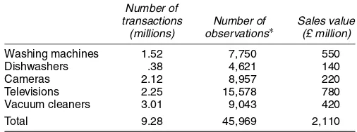
The empirical work uses monthly 1998 “scanner” data for five products: washing machines, dishwashers, television sets, cameras, and vacuum cleaners. In each month, all of the trans-actions from the bar-code readers (scanners) of retailers are aggregated for each model (“branded variety”) of the prod-uct in each of four outlet types to provide for each model in each month sold in each outlet type, unit values (“price”), sales volumes, and sales values. The scanner data also include for each model a unique model identifier and a set of variables on quality characteristics. Table 1 shows the dataset to be quite extensive, comprising nearly 46,000 observations (models in an outlet type in a month) made up from more than 9 billion transactions worth more than £2 billion. Details of the qual-ity characteristic sets for each product are given in Appen-dix B.
The analysis uses the scanner data to simulate the matched-model method. We start by taking a January fixed basket of all models of, say, washing machines in each of the four out-let types: chain stores, department stores, catalog stores, and independents. The unique identifier for each model in each out-let type allows us to identify in each subsequent month which
Table 1. Coverage of the Scanner Data
Number of
transactions Number of Sales value (millions) observations∗ (£ million)
Washing machines 1.52 7,750 550 Dishwashers .38 4,621 140 Cameras 2.12 8,957 220 Televisions 2.25 15,578 780 Vacuum cleaners 3.01 9,043 420 Total 9.28 45,969 2,110
∗Model of a product in an outlet type and month.
observations are matched (with January) models, newly intro-duced unmatched models, and old unmatched models to allow the decompositions in (15) and (18). The scanner data also in-clude an extensive variable set on quality characteristics for each model in each outlet type, which are also necessary for the decomposition in (15) and (18). Equations (15) and (18) show the extent of sample degradation and differences between hedonic-adjusted prices of matched, unmatched new, and un-matched old models in outlet types to be responsible for the bias; we examine these in turn in Sections 5 and 6. Although the empirical work is generally for all five products, in some instances, for the sake of brevity, the focus is on washing ma-chines for illustration.
5. IS THE SAMPLE DEGRADATION FROM MATCHING SUBSTANTIAL?
First, (15) and (18) show that if the number or sales share of unmatched models (hereafter “models” refers to models in an outlet type) in the sample is high, so too might the bias from estimates based on the matched sample. A necessary condition for significant bias from using matched pairs estimates is sig-nificant sample “degradation.” Table 2 shows that for matched models of washing machines, only 53% of models existing in January were still available in December for comparison, al-though such machines accounted for about 80% of their sales value in January. However, this January-to-December matched comparison of washing machines accounted for about 50% of the December sales value. There was a similar pattern for the other products, with falls in coverage to under two-thirds of the number of models in January but much smaller falls in the shares of January’s sales value attributed to those models still existing in December. By December 1998, the matched models covered less than 75% of December sales by value for dish-washers, vacuum cleaners, and cameras, but only about 50% for television sets and washing machines.
6. DO HEDONIC QUALITY–ADJUSTED MATCHED AND UNMATCHED PRICES DIFFER?
In this section we show that the prices of old unmatched mod-els, new unmatched modmod-els, and matched models are system-atically different, after controlling for hedonic characteristics. Equations (15) and (18) clearly show that differences between hedonic quality-adjusted prices for matched and old and new unmatched models were critical determinants of the extent and nature of any bias from using only matched models to estimate
Table 2. Summary of Coverage Results for Five Products
% of % of % of
January’s January’s current period’s observations∗ sales value sales value
Washing machines
∗Model of a product in an outlet type and month.
price changes. Hedonic regressions of the form given in (1) were estimated for bimonthly data on January (period 1) and in turn, each successive current montht,S(1)andS(t), for each of 2≤t≤12. The residualsεm for each model from each of the January (period 1) on current month (period t) compar-isons in 1998 [i.e., S(1)∪S(t)], are estimates of the price of
Table 3. Residuals and Leverage for Matched and Unmatched New and Old Models
Means
Residuals Leverage Unmatched Unmatched Matched Old New Matched Old New
Washing machines
OLS unweighted resid. .006 −.054 .009 .036 .068 .060 WLS∗unweighted resid. .011 −.068 .032 .041 .043 .055 Cameras
OLS unweighted resid. .015 −.077−.025 .055 .076 .081 WLS∗unweighted resid. −.070 −.184−.136 .063 .048 .047 Television sets
OLS unweighted resid. .006 −.032−.003 .015 .021 .022 WLS∗unweighted resid. −.040 −.113−.040 .017 .011 .018 Dishwashers
OLS unweighted resid. .001 −.008 .003 .033 .043 .049 WLS∗unweighted resid. .017 .006 .030 .040 .019 .033 Vacuum cleaners
OLS unweighted resid. .013 −.098 .019 .017 .022 .020 WLS∗unweighted resid. −.077 −.201−.042 .020 .007 .015
∗The weighting is by sales value shares as described in Section 2.2.
each model after adjustments for quality differences. The un-weighted means of the residuals, ε¯1 :mt =
mε1 :mt/N(m), and weighted means,wε¯m1 :t=
msmεm1 :t/
msm, were calculated for matched,m∈S(1∩t); unmatched old, m∈S(1¬t), and unmatched new, m∈ S(t¬1), observations, to see how the mean matched and unmatched quality-adjusted prices compare, and then averaged over the 11 month-on-month comparisons (i.e.,ε¯¯m=tε¯1 :mt/11 and
twε¯1 :mt/11) to provide summary results in Table 3.
We were also concerned that unmatched observations may have more or less leverage and influence in determining the re-gression estimates than warranted by their (equal) ordinary least squares (OLS) or WLS weights (see App. A). The primary rea-son for our use of weights in the WLS estimator is for the index to be representative of sales value shares (Diewert 2002), and undue leverage may adversely affect the weights. The means of leverage statistics [eq. (A.2) in App. A] were calculated for each January on current period comparison for matched, un-matched old, and unun-matched new models, and the annual aver-ages were summarized for all products in Table 3 as the average of the 11 monthly comparisons, that is,h¯1 :mt=
mh1 :mt/N(m) andh¯¯m=th¯1 :mt/11. The residuals and leverage were calcu-lated using both OLS and WLS (weighted by sales share, as defined in Sec. 3.1) estimators.
It is clear from Table 3 that for all products and both esti-mators, the average of the residuals from old unmatched obser-vations fellbelowthe average residuals of the matched ones. Furthermore, in all cases the average of the residuals for un-matched new models fell above the average for unmatched old ones. For washing machines, dishwashers, vacuum clean-ers, and television sets (WLS), the average of the residuals for the new unmatched models was equal to or exceeded those of their matched counterparts, and for cameras and televisions sets (OLS), the new unmatched model’s residuals on average ex-ceeded those of the old unmatched ones, but not the average residuals of the matched models. There is thus a clear
eral pattern of lower-than-average quality-adjusted prices for old unmatched models and higher-than-average prices for new unmatched quality-adjusted prices. Leverage effects were for the most part higher on average for unmatched new and old models than for matched models.
Tests of differences between quality-adjusted prices for matched and unmatched new and old models can be under-taken by estimating equation (1) for a comparison between the initial month January and each of the current months,t [i.e., S(1)∪S(t)for 2≤t≤12], but to include in the specification of (1) two further dummy variables. The first of these takes the value 1 if the observation present in periodt was not present in period 1 (i.e., is an unmatchednewmodel) and 0 otherwise. The second dummy variable takes the value 1 if the observa-tion present in period 1 is not present in period t (i.e., is an unmatchedoldmodel) and 0 otherwise. The coefficients are es-timates of how unmatched old and unmatched new prices differ from their benchmarked matched observations when adjusted for quality and time.
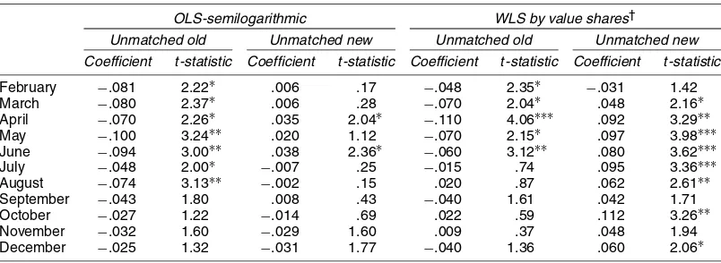
The results presented in Table 4 are for washing machines only for illustration and are given for the coefficients on the foregoing dummy variables for the new and old unmatched models, although the regressions included all variables in Ap-pendix B. The regression equations fitted well by the usual criteria with a mean R2 for the 11 comparisons of .85 and a standard deviation of a mere .0022. Full regression results for all products are available from the authors. It is appar-ent from Table 4 that there is a consistappar-entnegativeimpact on price, after adjusting for quality, for unmatchedold observa-tions in each month, generally statistically significant at the 5% level, and this holds regardless of whether an OLS or a WLS estimator is used. There is also evidence of apositive dif-ference between unmatched new models and (the benchmark) matched ones, after adjusting for quality, although it is less clear. The OLS semilogarithmic results found only two sig-nificant coefficients at the 5% level and they were both pos-itive. Yet the WLS counterpart had positive differences from the benchmarked matched models in all months, with these dif-ferences being statistically significant for 6 months. New en-trants seem to have higher quality-adjusted prices than matched ones.
7. WHAT IS THE NATURE AND EXTENT OF THE INDEX NUMBER BIAS IF ONLY MATCHED
ITEMS ARE USED?
7.1 Factors Determining the Bias
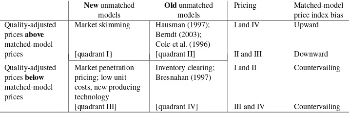
Equations (15) and (18) showed that sample degradation (es-tablished in Sec. 5) and differences in the (quality-adjusted) prices of unmatched new, unmatched old, and matched mod-els (established in Sec. 6) can lead to bias in matched-model price indexes. The nature and extent of such bias depends on the frequency with which manufacturers turn over their models and the pricing strategy that retailers use over the life cycle of the models (Parker 1992). It can be deduced from (15) and (18) that if the quality-adjusted prices of new unmatched models in, say, periodt=2, are higher than their matched counterparts in period 2, and if the quality-adjusted prices of old unmatched models in period 1 are lower than their matched counterparts in period 1, then there will be a largerfall in the matched mod-els index between periods 1 and 2 compared with a hedonic index that uses all of the data. Similarly, if the quality-adjusted prices of unmatched new models, arebelowmatched ones in pe-riod 2, and the quality-adjusted prices of old models areabove matched ones in period 1, then there will be asmallerfall in the matched-model index compared with a hedonic index that uses all of the data. The nature and extent of the matched-model in-dex bias thus depends on the pricing strategy adopted for new and old models. Indeed, if hedonic-adjusted prices are consis-tently above or consisconsis-tently below average for unmatched new andold models, then some of the bias will cancel out.
The case for old unmatched models having below-average quality-adjusted prices is based on an inventory-clearing argu-ment. For an old model near or at the end of its life cycle, re-tailers want to clear out the remaining inventory from both their warehouses and store shelves so they have room to stock and display the replacement model. They do not wish the old model to cannabalize some of the sales of the new model, which may well have a higher price (profit) margin. The extent of any such cannibalization will depend on the cross-price elasticities be-tween the new and old models (Bresnahan 1997). This inven-tory clearing argument is noted in quadrant IV of Figure 1.
Table 4. Hedonic Regression Coefficients (semilogarithmic) for Unmatched New and Old Dummy Variables
OLS-semilogarithmic WLS by value shares†
Unmatched old Unmatched new Unmatched old Unmatched new Coefficient t-statistic Coefficient t-statistic Coefficient t-statistic Coefficient t-statistic
February −.081 2.22∗ .006 .17 −.048 2.35∗ −.031 1.42 March −.080 2.37∗ .006 .28 −.070 2.04∗ .048 2.16∗ April −.070 2.26∗ .035 2.04∗ −.110 4.06∗∗∗ .092 3.29∗∗ May −.100 3.24∗∗ .020 1.12 −.070 2.15∗ .097 3.98∗∗∗ June −.094 3.00∗∗ .038 2.36∗ −.060 3.12∗∗ .080 3.62∗∗∗ July −.048 2.00∗ −.007 .25 −.015 .74 .095 3.36∗∗∗ August −.074 3.13∗∗ −.002 .15 .020 .87 .062 2.61∗∗ September −.043 1.80 .008 .43 −.040 1.61 .042 1.71 October −.027 1.22 −.014 .69 .022 .59 .112 3.26∗∗ November −.032 1.60 −.029 1.60 .009 .37 .048 1.94 December −.025 1.32 −.031 1.77 −.040 1.36 .060 2.06∗
∗∗∗,∗∗, and∗denote statistical significance at a .1%, 1%, and 5 % level for two-tailedt-tests. †The weighting is by sales value shares, as described in Section 2.2.
Newunmatched Oldunmatched Pricing Matched-model
models models price index bias
Quality-adjusted pricesabove matched-model prices
Market skimming
[quadrant I}
Hausman (1997); Berndt (2003); Cole et al. (1996) [quadrant II]
I and IV
II and III
Upward
Downward
Quality-adjusted pricesbelow matched-model prices
Market penetration pricing; low unit costs, new producing technology [quadrant III]
Inventory clearing; Bresnahan (1997)
[quadrant IV]
I and II
III and IV
Countervailing
Countervailing
Figure 1. Factors Determining the Bias.
New and old models may coexist for some time and the case for existing models having theirpostentrypricesincreased af-ter the introduction of a new model is of inaf-terest. In principle, our focus is on unmatched old items no longer available for the matched price comparison, and hence they have no postentry prices. However, the logic behind such postentry pricing ap-plies to a pricing strategy for a multiproduct firm that antici-pates the introduction of a new model. Hausman (1997) argued that a multiproduct monopolist can increase the prices of ex-isting models because some of the demand for exex-isting mod-els that would usually be lost to competitors, due to the price increase, will now not go to the competitor’s products (an as-sumption upon which the existing prices were set) but will go instead to the firm’s new model. The new model will canna-balize some of the existing model’s sales that would otherwise be lost due to the price increase in the existing model (Fig. 1, quadrant II). Bresnahan (1997) was critical of this position, ar-guing that any such effect may be outweighed by the need to cut the prices of the existing models to prevent the existing model’s sales cannibalizing sales of the new, more profitable model (Fig. 1, quadrant IV). Berndt, Ling, and Kyle (2003) also examined postentry prices of existing models and showed that prices of old branded pharmaceutical drugs can increase after the expiration of a patent and introduction of new generic mod-els. This is because of price discrimination with some market segments remaining with particularly strong preferences for the old models willing to pay higher prices (Fig. 1, quadrant IV). Cole et al. (1986), in their study of computer processors and disk drives, found that postentry quality-adjusted prices of old models may be higher than those of new models (Fig. 1, quad-rant II), but that this was a short-run phenomena:
. . .the introduction of products embodying new technology leads initially to multiple prices with the products based on “non-best” technologies selling for more. The prices for older products decline rapidly until they either match the quality-adjusted price of products based on the new technology or the prod-ucts disappear. The claim that improved technology leads to reduced costs and, hence, to a lower quality-adjusted price is consistent with a competitive market-place in which the only quality-adjusted price (the “best”) ultimately prevails. It was found that in many cases price reductions permit an older technology to compete with a newer one for a limited time, but as the new technology be-comes diffused, its own age-related cost and price reductions eventually drive the older technology out of production. The evidence presented here suggests that prices reflect this process of adjustment and that equilibrium is not reached within a period as short as 1 year (Cole et al. 1986, p. 47).
Our findings for old unmatched models, however, are con-sistent with the market clearing of the old models to minimize cannabalization, as might be expected for electrical consumer durables, rather than postentry price increases.
New models may haveaboveaverage quality-adjusted prices in their period of introduction because firms “price-skim” mar-ket segments willing to pay a premium for the new model over and above that due to its improved quality (Fig. 1, quadrant I). Indeed, marketing texts, such as that of Kotler and Armstrong (2001), advocate price-skimming as one of two “new prod-uct” pricing, strategies. The alternative strategy is “market-penetration” pricing, for which a low initial price is set for a new model to attract a large number of buyers quickly to win market share and take advantage of falling costs due to scale economies. Such pricing may initially be possible because the new model is based on new, lower-cost components that can provide a feature set comparable to existing models, but at a lower price point. In either event quality-adjusted prices of new models may havebelowaverage prices (Fig. 1, quadrant III).
Figure 1 summarizes these positions. Consider the right side of (15). The first summation is for matched models. The second summation is for new models,m∈S(2¬1), which has a posi-tive sign and potential upward bias to the matched-model index. The third summation is for old models, m∈S(1¬2), which have a potential negative, downward bias. The combination of above-average prices for new models in I and below-average prices for old models in III leads to an overall net upward bias. Similar pricing in quadrants II and III lead to matching-model indexes that are biased downward. However, pricing in quad-rants I and II lead to an indeterminate bias, with countervailing positive bias from the new above-average priced models and negative bias from old average-priced models. The bias from pricing in quadrants III and IV is also indeterminate, with pos-itive bias from the new above-average priced old models and negative bias from the old below-average priced models.
It is possible to say something about the likely pricing strate-gies of different products. Consider the case of digital cam-eras compared with film-based camcam-eras. Given the current differential in product costs for the two technologies and where the two categories are in their respective life cycles, we can speculate that relatively greater effort is likely to be placed on R&D in new models that reduces unit costs for digital cameras compared with R&D in film-based camera models that reduces unit costs. Products in a mature stage of their category life cy-cle, where R&D development is relatively small and product enhancing, as opposed to cost reducing, may be more likely to have above-average quality-adjusted prices for new mod-els. The products considered in this study take this form, and the results are consistent with this. The foregoing analysis has
demonstrated how the nature and the extent of bias from us-ing matched models is dictated by the pricus-ing and production strategies of the retailers and manufacturers. Our findings in Sections 5 and 6 are consistent with the price skimming of new models and inventory clearing of old models, and thus lower index numbers for matched hedonic indexes than models that rightfully use all of the data.
7.2 Empirical Results on the Bias
Table 5 provides the results for hedonic price index num-bers for washing machines using different samples of observa-tions; matched models with unmatched old models, matched models with unmatched new models, and matched models with unmatched old and new models—all of the data. In this way we can see how the sample selection affects the results for the index. The results for only matched samples and all of the data are summarized for other products in Table 6 for brevity, al-though they are available from the authors on request. The he-donic indexes for all of Tables 5 and 6 are estimated as exp(αt), whereαtare the coefficients on the time dummy variables in (1) that were estimated as direct fixed base comparisons between January 1998 and each month in question. Adjustments to the coefficient on the semilogarithmic form of half the squared standard error following Teekens and Koerts (1972) were neg-ligible given the small standard errors.
Table 5 shows first that the estimated quality-adjusted price index for washing machines fell faster when based on the matched samples than when based on all of the data, the matched and unmatched samples, with this result holding for both estimators (although with a single exception, October
WLS). Similar results held for linear forms; the results are available from the authors. Second, the differences between the estimates from the different samples were quite marked. By December 1998, quality-adjusted prices were estimated to have fallen by exp(−.099) 9.4% for matched data compared with an estimated fall of exp(−.070)=6.8% for all of the data. The exclusion of unmatched data can be seen to seri-ously overstate these price falls. Third, the index using matched plus unmatched new and old models does not fall as fast as the index using matched plus just new or matched plus just old models. The combined effect of lower old prices and higher new prices leads to lower overall falls. For example, for the WLS estimator in Table 5, the index using all of the data fell over the 12 months by only exp(−.061)=5.9% compared with falls of exp (−.089)=8.5% for the index using matched and old unmatched models, exp(−.077)=7.4% for the index us-ing matched and new unmatched models, but a higher fall of exp(−.095)=9.7% for just the matched model.
Table 6 provides the results for OLS and WLS hedonic in-dexes for all products using the full sample and the matched sample. The results are quite clear. Quality-adjusted hedonic in-dexes fell further for cameras, television sets, vacuum cleaners, and washing machines when just the matched data were used than when both the unmatched and matched data were used. The only exception was dishwashers, for which the OLS in-dexes fell at the same rate and the WLS inin-dexes were slightly lower when all of the data were used. In Table 3 the resid-uals for dishwashers for WLS were higher for OLS models than matched ones, giving rise to this exceptionally different pattern.
Table 5. Hedonic Regression (semilogarithmic) Coefficients for Dummy Variable on Time for Matched and Unmatched Samples: Washing Machines
Matched plus old and new Matched plus Matched plus Matched unmatched–all the data unmatched old unmatched new
Coefficient Coefficient Coefficient Coefficient
on time dummy t-statistic on time dummy t-statistic on time dummy t-statistic on time dummy t-statistic
OLS
February .008 .75 .017 1.52 .016 1.50 .008 .77 March .000 .02 .011 .96 .010 .79 .001 .08 April −.010 .83 .010 .84 .001 .07 −.001 .08 May −.013 1.16 .013 1.16 .006 .54 −.005 .45 June −.050 4.40∗∗∗ −.015 1.29 −.033 2.63∗∗ −.033 3.01∗∗ July −.055 4.07∗∗∗ −.034 2.36∗ −.012 3.15∗∗ −.049 3.40∗∗∗ August −.059 4.87∗∗∗ −.024 2.17∗ −.036 2.83∗∗ −.048 4.34∗∗∗ September −.070 5.21∗∗∗ −.034 2.69∗∗ −.049 3.34∗∗∗ −.053 4.14∗∗∗ October −.078 4.94∗∗∗ −.049 3.30∗∗ −.055 3.35∗∗∗ −.066 4.34∗∗∗ November −.080 6.02∗∗∗ −.054 4.20∗∗∗ −.056 3.85∗∗∗ −.076 5.59∗∗∗ December −.099 7.63∗∗∗ −.067 5.48∗∗∗ −.070 5.39∗∗∗ −.089 6.84∗∗∗ WLS by value shares∗
February −.008 .92 −.008 .92 −.007 .81 −.008 1.04 March −.009 1.17 −.007 .83 −.009 1.15 −.007 .86 April −.020 2.34∗ −.007 .78 −.019 2.21∗ −.009 .93 May −.032 3.53∗∗∗ −.015 1.50 −.031 3.45∗∗∗ −.017 1.72 June −.055 5.76∗∗∗ −.040 3.93∗∗∗ −.053 5.82∗∗∗ −.040 4.10∗∗∗ July −.072 4.53∗∗∗ −.051 3.67∗∗∗ −.070 4.57∗∗∗ −.053 3.65∗∗∗ August −.064 6.08∗∗∗ −.050 4.30∗∗∗ −.064 6.07∗∗∗ −.050 4.50∗∗∗ September −.067 6.68∗∗∗ −.050 4.45∗∗∗ −.064 6.62∗∗∗ −.060 5.23∗∗∗ October −.083 6.13∗∗∗ −.055 3.65∗∗∗ −.084 5.46∗∗∗ −.059 4.32∗∗∗ November −.084 7.86∗∗∗ −.063 5.64∗∗∗ −.084 7.95∗∗∗ −.070 6.04∗∗∗ December −.093 9.40∗∗∗ −.061 4.60∗∗∗ −.089 9.29∗∗∗ −.077 6.39∗∗∗
∗The weighting is by sales value shares as described in Section 2.2.
Table 6. Hedonic (semilogarithmic) Indices for Matched and All Data, January 1998=1.000
Matched data All data
WLS by WLS by
OLS value shares∗ OLS value shares∗
Cameras
February .986 .986 .979 .984 March .971 .975 .973 .975 April .953 .956 .948 .953 May .922 .938 .947 .940 June .920 .927 .921 .925 July .913 .911 .925 .909 August .898 .894 .930 .900 September .874 .873 .912 .874 October .876 .870 .905 .871 November .856 .867 .882 .867 December .853 .848 .878 .849 Dishwashers
February 1.010 1.003 1.012 1.003 March 1.005 1.001 1.005 .998 April .991 .991 1.002 .990 May .986 .978 .980 .976 June .963 .953 .976 .956 July .963 .964 .959 .964 August .948 .949 .966 .952 September .941 .938 .951 .937 October .936 .944 .921 .941 November .910 .922 .930 .918 December .932 .928 .932 .925 Washing machines
February 1.008 .992 1.017 .992 March 1.000 .990 1.012 .993 April .990 .980 1.010 .992 May .988 .969 1.013 .985 June .949 .946 .985 .962 July .946 .930 .966 .950 August .943 .938 .976 .953 September .932 .935 .966 .955 October .925 .920 .953 .947 November .919 .919 .948 .939 December .906 .911 .936 .940 Television sets
February .994 .996 .991 .997 March .979 .989 .980 .990 April .969 .982 .976 .990 May .954 .978 .971 .982 June .929 .963 .940 .965 July .921 .958 .939 .964 August .913 .939 .938 .951 September .885 .921 .876 .934 October .875 .905 .865 .919 November .854 .891 .883 .908 December .843 .876 .871 .896 Vacuum cleaners
February .997 .998 1.021 1.000 March .988 .994 1.018 .997 April .984 .992 1.012 .992 May .975 .992 1.001 .995 June .974 .982 1.008 .987 July .958 .962 .992 .966 August .943 .954 .979 .957 September .909 .945 .965 .951 October .897 .933 .967 .942 November .894 .938 .961 .954 December .902 .937 .961 .953
∗The weighting is by sales value shares as described in Section 2.2.
8. STRATEGIES FOR REDUCING THE BIAS
A strategy for reducing sample degradation, and thus the matched-model bias, is to rotate (update) the sample more fre-quently, say on a biannual, quarterly, or monthly (chained)
ba-Table 7. Illustration of Matching and Approaches to Quality Adjustment
Model January February March
1 p1Jan p1Feb p1Mar
2 p2Jan p2Feb
3 p3Mar
4 p4Feb p4Mar
5 p5Jan p5Feb p5Mar
6 p6Jan p6Feb
7 p7Mar
sis. Consider Table 7, which shows prices for seven models over the 3 months January to March. A direct comparison be-tween matched prices bebe-tween January and March would use only models 1 and 5. If the sample were rotated monthly, then a chained index for January compared with March would be made from the product of two links, January and February and February and March. For the first link, models 1, 2, 5, and 6 would be used, but notp4Feb;because the February to March
link matched price comparisons are possible only for models 1, 4, and 5, and pricesp2Feb,p3Mar,p6Feb, andp7Marwould not be
used. More frequent sample rotation including monthly chain-ing thus increases the use of sample information compared with direct fixed base comparisons, but does not use all of the price information. We noted in Section 3 the advocacy of chaining arising from the ACD study on the basis of it providing sim-ilar results to the more complicated hedonic indexes. In Sec-tion 3 we also saw how the ACD approach had an equivalence to the matched-model method, and we see here how chaining may still not use all of the data and thus lead to possible bias. Chaining also has the disadvantage that when prices oscillate around a trend, the price index may drift (Forsyth and Fowler 1981; Szulc 1983).
In Table 8 for washing machines, we consider the coverage of the matched sample with sample rotation conducted on bian-nual, quarterly, and then monthly (chained) bases. The cov-erage relates to the percentage of the current month’s sales value captured in the matching of prices between the reference month (January) and the current month. For example, for bian-nual sample rotation, about 80% of the sales value of models sold in August was from matched models that were also avail-able in June. Tavail-able 8 shows the use of biannual sample rota-tion improved the coverage of the matching to at worst a little over 70%, compared with 48.2% when rotating annually— a substantial improvement. Table 8 shows that upgrading the rotation to a quarterly basis further improved coverage to an at worst 76.7% (September) and monthly chaining to 83.3% (July). The average coverage over the 12 months for the bian-nual, quarterly, and monthly chained procedures were 73.5%, 79.8%, and 86.8%, compared with 67.7% for the annual sam-ple rotation.
An alternative strategy to the use of sample rotation to curtail the sample degradation from matching is to select replacement models if older models go missing. If a replacement model is not directly comparable in quality to the missing model, then a hedonic regression may be used to estimate the effect of the quality difference on price and remove this from the price comparison. This approach was called “patching” by Silver and Heravi (2003). Triplett (2004) provided a thorough ac-count of such approaches. We estimated hedonic regressions in
Table 8. Number of Observations and Sales Value Percentages Used Under Sample Rotation: Washing Machines
January sample without rotation:
Sample rotation
Biannual Quarterly Monthly chained % of current % of current % of current % of current period’s sales value period’s sales value period’s sales value period’s sales value
February 97.1 97.06 97.06 97.06 March 91.1 91.06 91.06 91.88 April 81.8 81.79 94.86 94.86 May 76.6 76.62 91.11 97.59 June 72.9 72.90 86.34 96.83 July 64.2 83.33 83.33 83.33 August 57.5 80.31 80.31 98.80 September 54.2 76.71 76.71 98.56 October 51.6 75.25 86.62 86.62 November 49.4 75.74 87.09 98.85 December 48.2 71.08 83.13 97.72
each month and then identified missing unmatched models and their nearest replacements. The replacement models were de-termined by first undertaking a search for the best match within each outlet type in each month undertaking a search for the best match by matching first by brand, then, in turn, by type, width, and spin speed (see App. B). If more than one replacement model was found, then the replacement was selected according to the highest sales value. The subset of thek characteristics that distinguished the old missing and replacement new models was ascertained, and the coefficients from the hedonic equa-tions were applied to the difference in the values of the char-acteristics. This was done to first correct the new model’s price to adjust it to the old model’s characteristics. This adjusted new price in the current period was compared to the old price in the reference period. Then a second similar procedure was under-taken to correct the old model’s price to make it comparable to the new one, and an estimate of the quality adjusted price change was made on this basis. A geometric mean was taken of the two resulting estimates, and this was used to measure the model’s price change (see Triplett 2004). Note that replace-ment patching does not cover all of the sample degradation. In Table 8, in March models 2 and 6 are missing, but only two of the three model prices (3, 4, and 7) are used as replacements.
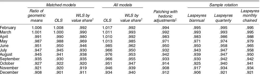
Table 9 compares the results of indexes for washing ma-chines using only matched models, all models with replace-ment patching, and more frequent sample rotation for matching. The first three columns use matched data only and are for fixed base comparisons: the simple geometric mean of matched price changes; the OLS estimator exp(αt), whereαtis the coefficient on the time dummy variable in (1); and the WLS estimator us-ing sales share weights as described in Section 2.2. The first two columns are equally weighted indexes and provide similar results 9% to 10% fall. The weighted estimator found a lower fall in prices at 8.9%. Yet when all of the data—matched and unmatched—were used in the fourth and fifth columns of ta-bles, we have even lower falls in prices: 6.6% without weights and 6.0% with weights. As predicted from (15) and (18), the combined effect of the relatively low unmatched old models and high priced unmatched new models combine to limit the fall in prices of the matched models. So do our strategies of patch-ing replacement models with hedonic adjustments and sample rotation help? The patching described at the start of this sec-tion when used in a weighted index led to a fall similar to its matched WLS counterpart: falls of 8.8% compared with 8.9%. With patching some of the new models with their above-average (hedonic-adjusted) prices are excluded from the sample, be-cause new models can be brought in as substitutes only when a
Table 9. Results of Indexes∗Using Matching, Patching, and Sample Rotation: Washing Machines
Matched models All models Sample rotation
Ratio of Patching with
hedonic adjustments‡
Laspeyres
geometric WLS by WLS by Laspeyres Laspeyres monthly
means OLS value share† OLS value share† biannual quarterly chained
February 1.006 1.008 .992 1.017 .992 .994 .995 .995 .995 March 1.001 1.000 .990 1.011 .993 .992 .993 .993 .995 April .991 .990 .980 1.010 .992 .983 .983 .986 .988 May .987 .988 .969 1.013 .985 .971 .971 .974 .979 June .951 .950 .946 .985 .962 .950 .950 .958 .965 July .947 .945 .930 .966 .950 .932 .943 .947 .958 August .945 .941 .938 .976 .953 .942 .939 .947 .950 September .935 .930 .935 .966 .955 .933 .930 .942 .942 October .927 .922 .920 .951 .947 .914 .925 .940 .941 November .921 .920 .919 .946 .939 .908 .917 .934 .934 December .908 .901 .911 .934 .940 .912 .906 .921 .921
∗OLS and WLS dummy variable regression estimates use a semilogarithmic form and include an adjustment to the coefficient on the dummy for time in (1) of half the squared standard error following Teekens and Koerts (1972).
‡WLS with forced replacements quality-adjusted using hedonic coefficients. †The weighting is by sales value shares as described in Section 2.2.
model is no longer sold. Quarterly and monthly (chaining) sam-ple rotation went some way toward reduce the bias, with a price fall of 7.9% for a weighted index compared with 6.0% using all of the data. However, hedonic indexes using all of the data remained preferable on the grounds of sample selection.
9. CONCLUSIONS
The analytical models developed in Section 2 provide de-compositions of quality-adjusted price changes into matched, unmatched old, and unmatched new components, thus allow-ing a formal identification of the nature and extent of bias from using the matched-model method. A necessary condition for matched-model sample selectivity bias is that the product mar-ket has a high model turnover, and thus the matching of models leads to sample degradation. We found evidence of substantial sample degradation; for washing machines, for example, in the January to December price comparison, only 53% of models existing in January were still available in December for com-parison, although such machines accounted for about 80% of the sales value in January. However, the matched sample of washing machines accounted for less than 50% of the Decem-ber sales value.
The nature and extent of the bias from using the matched-model method was found to depend on the pricing policies and supply strategies of retailers and manufacturers for old unmatched retired models and newly introduced models. The empirical work found patterns of relatively high (hedonic-adjusted) prices for new unmatched models, consistent with price skimming, and relatively low (hedonic-adjusted) prices of old unmatched models, consistent with inventory clearing. These findings resulted in a substantial matched-model down-ward bias for the five electrical consumer durables studied. For example, for washing machines, the (weighted) fall of 6.0% using all of the data was overestimated at 8.9% using matched models. The empirical impact of strategies to amelio-rate the bias were examined. Such stamelio-rategies included the use of replacement models with hedonic adjustments for missing old models and sample rotation on a more regular biannual, quarterly, and monthly (chained) basis. Quarterly and monthly (chained) rotated indexes went some way toward alleviating the bias, but hedonic indexes that use all of the data are advocated. The analytical model from Section 2 was also used in Sec-tion 3 to shed some light on the influential ACD results. It was shown in Section 3 that for fixed base comparisons, the ACD model is equivalent to a matched-model method. The ACD ar-ticle has been cited by Greenspan as justification for the chained (matched-models) approach as against hedonic indexes because of (with good data) the similarity of their results and the sim-plicity of the former. In the empirical section we found that the similarity of hedonic and chained matched indexes need not hold.
ACKNOWLEDGMENTS
Different versions of this work have benefited from useful suggestions. In particular, the authors thank Erwin Diewert, University of British Columbia, who helpfully provided rig-orous derivations of results in a previous working version of
this manuscript. These contributed greatly to the article. Helpful comments were also received from Ana Aizcorbe (BEA), Ernst Berndt (MIT), Ellen Dulberger (IBM), Rob Feenstra (Univer-sity of California, Davis), David Fenwick (ONS), Vitor Gaspar (ECB), John Greenlees (BLS), Johannes Hoffman (Deutches Bundesbank), Brent Moulton (BEA), Ariel Pakes (Harvard University), Jack Triplett (Brookings Institution), Ralph Turvey (LSE), and anonymous referees. The usual disclaimers apply. The views expressed in this article are those of the authors and should not be attributed to their organizations. Some of the work was undertaken while an ASA/NSF Senior Research Fel-low at the Bureau of Labor Statistics, Washington DC.
APPENDIX A: MEANS FOR RESIDUALS AND LEVERAGE FOR MATCHED, UNMATCHED OLD,
AND UNMATCHED NEW SAMPLES
An OLS vector ofβestimates is a weighted average of the individualpelements, the prices of individual models, and the
Zexplanatory variables,
β=(ZTZ)−1ZTp. (A.1) Here(ZTZ)−1ZTare the weights given to the prices, with some observations likely to have more influence than others. Our con-cern is with the effect of adding a, for simplicity, single new unmatched observationmto the regression estimate in periodt, although via (15) and (18), the extension to several new obser-vations and a weighted estimator is straightforward.
Following Davidson and McKinnon (1993), we compareβˆ with βˆ(m) where the latter is an estimate of β if OLS were used on a sample omitting the period t unmatched observa-tion, hereafter—the mth observation. We distinguish between the leverage of the mth observation, hm, and its residual, εm. An influential observation may, for example, have high lever-age, that is, influence on at least one element ofβˆ but a smaller impact on εm, or it may have little leverage but have a high residual. The leverage for observationmis given by:
hm=Zm(ZTZ)−1ZTm, where 0≤hm≤1, (A.2) and the difference between the hedonic coefficients with the mth observation omitted and included is given by
ˆ
β(m)− ˆβ= −
1 1−hm
(ZTZ)−1ZTmεm. (A.3)
APPENDIX B: QUALITY CHARACTERISTICS INCLUDED IN THE HEDONIC REGRESSIONS
Washing machines: (i) Manufacturer (make)—dummy vari-ables for about 20 makes; (ii) types of machine: 5 types— top-loader; twin tub; washing machine (WM); washer dryer (WD) with and without computer; WD with/without con-densers; (iii) drying capacity of WD; (iv) height of machine in cm; (v) width; (vi) spin speeds; 5 main—800 rpm, 1000 rpm, 1100 rpm, 1200 rpm, and 1400 rpm; (vii) water consumption; (viii) load capacity; (ix) energy consumption (kWh per cycle); (x) free standing, built-under and integrated; built-under not in-tegrated; built-in and inin-tegrated; (xi) vintage; (xii) outlet-type: chain stores, department stores, independents, catalogues.
Dishwashers: (i) Manufacturer (make)—dummy variables for about 22 makes; (ii) type of machine; 4 types—built-under, built-under integrated; table top; free standing; (iii) with micro chip; (iv) width; (v) height; (vi) kWh per cycle; (vii) number of plates; (viii) number of programmes; (ix) partly integrated; non-integrated switch panel; (x) water consumption; (xi) stain-less steel; (xii) vintage; (xiii) outlet-type: chain stores, depart-ment stores, independents, catalogues.
Vacuum cleaners: (i) Manufacturer (make)—dummy vari-ables for about 29 makes; (ii) wattage; (iii) integrated/separate; (iv) remote control; (v) cord rewind; (vi) shampoo; (vii) speed control; (viii) soft-hard box; (ix) type of machine: 6 types— cylinder; upright; wet/dry; steam; hand stick; rechargeable; (x) outlet-type: chain stores, department stores, independents, catalogues.
Cameras: (i) Manufacturer (make)—dummy variables for about 25 makes; (ii) type of camera: 6 types—135; roll film 120/220; instant; camera 110; disc; APS; (digital excluded); (iii) view system: single lens reflex (SLR); viewfinder; bridge; (iv) exposure system: manual; aperture; programme; (v) lens: bifocal; fixed; zoom; (vi) water resistant; (vii) compact zoom range: less than 60; 1–80; 1–90; 1–105; 6–115; 115 mm and more; (viii) panoramic (APS); (ix) dateback (APS); (x) ti-tles; (xi) film specifications (APS); (xii) camera specifications (APS); (xiii) mid roll change (APS); (xiv) medium format SLR 6×6; (xv) DX coding; (xvi) automatic loading (drop in); (xvii) motor advance; (xix) mini (108 mm or less); (xx) auto fo-cus; (xxi) built-in flash; (xxii) red eye reduction; (xxiii) vintage; (xxiv) outlet-type: specialized stores; independent chemists; nonspecialized.
Television sets: (i) manufacturer (make)—dummy variables for about 50 makes; (ii) size of screen—dummy variables for about 15 screen sizes; (iii) Nicam stereo sound; (iv) 6 tuner types; (v) teletext—fastext, no text retrieval system; (vi) picture tube—flat screen technology; (vii) monitor style; (viii) dolby system; (ix) wide screen; (x) s-vhs socket; (xi) satellite tuner; (xii) digital; (xiii) vintage—year model first introduced; (xiv) outlet type: chain stores, department stores, independents, catalogues.
[Received February 2003. Revised July 2004.]
REFERENCES
Aizcorbe, A., Corrado, C., and Doms, M. (2000), “Constructing Price and Quantity Indexes for High-Technology Goods,” Industrial Output Section, Division of Research and Statistics, Board of Governors of the Federal Re-serve System, July.
Arguea, N. M., Hsiao, C., and Taylor, G. A. (1994), “Estimating Consumer Preferences Using Market Data: An Application to U.S. Automobile De-mand,”Journal of Applied Econometrics, 9, 1–18.
Balk, B. M. (2002), “Price Indexes for Elementry Aggregates: The Sam-pling Approach,” Statistics Netherlands Research Paper, No. 0231, Vooburg, The Netherlands: Statistics Netherlands.
Berndt, E. R., Griliches, Z., and Rappaport, N. J. (1995), “Econometric Es-timates of Price Indexes for Personal Computers in the 1990s,”Journal of Econometrics, 68, 243–268.
Berndt, E. R., Ling, D., and Kyle, M. K. (2003), “The Long Shadow of Patent Expiration: Generic Entry and Rx to OTC Switches,” inScanner Data and Price Indexes, eds. M. Shapiro and R. Feenstra, CRIW and NBER, Chicago: University of Chicago Press, pp. 229–273.
Boskin, M. J. (chair), Dullberger, E. R., Gordon, R. J., Griliches, Z., and Jorgenson, D. W. (1996),Final Report of the Commission to Study the Con-sumer Price Index, U.S. Senate Committee on Finance, Washington, DC: U.S. Government Printing Office.
Bresnahan, T. F. (1997), “Comment,” inThe Economics of New Goods, eds. T. F. Bresnahan and R. J. Gordon, NBER and CRIW, Chicago: University of Chicago Press, pp. 237–247.
Cole, R., Chen, Y. C., Barquin-Stolleman, J. A., Dulberger, E., Helvacian, N., and Hodge, J. H. (1986), “Quality-Adjusted Price Indexes for Computer Processors and Selected Peripheral Equipment,” Survey of Current Busi-nesses, 65, 41–50.
Committee of National Statistics, Schultze, C. L., and Mackie, C. (eds.) (2002),
At What Price? Conceptualizing and Measuring Cost-of Living and Price Indexes, Washington, DC: National Academy Press.
Davidson, R., and MacKinnon, J. G. (1993), Estimation and Inference in Econometrics, Oxford, U.K.: Oxford University Press.
Diewert, W. E. (1976), “Exact and Superlative Index Numbers,”Journal of Econometrics, 4, 114–145.
(1978), “Superlative Index Numbers and Consistency in Aggregation,”
Econometrica, 46, 883–900.
(2001), “Hedonic Regressions: A Consumer Theory Approach,” mimeo, University of British Columbia, Dept. of Economics.
(2002), “Hedonic Regressions: A Review of Some Unresolved Issues,” mimeo, University of British Columbia, Dept. of Economics.
(2003), “Hedonic Regressions: A Consumer Theory Approach,” in
Scanner Data and Price Indexes, eds. R. C. Feenstra and M. D. Shapiro, Chicago: University of Chicago Press, pp. 317–348.
Dulberger, E. R. (1989), “The Application of an Hedonic Model to a Quality-Adjusted Price Index for Computer Processors,” inTechnology and Capital Formation, eds. D. Jorgenson and R. Landau, Cambridge, MA: MIT Press. Forsyth, F. G., and Fowler, R. F. (1981), “The Theory and Practice of Chain
Price Index Numbers,”Journal of the Royal Statistical Society, Ser. A, 144, 224–247.
Greenspan, A. (2001), “The Challenge of Measuring and Modelling a Dynamic Economy,” Remarks at the Washington Economic Policy Conference of the National Association for Business Economics, Washington, DC, March 27, 2001.
Hausman, J. R. (1997), “Valuation of New Goods Under Perfect and Imper-fect Conditions,” inThe Economics of New Goods, eds. T. Bresnahan and R. J. Gordon, NBER, Chicago and London: University of Chicago Press, pp. 209–248.
Heravi, S., Heston, A., and Silver, M. (2003), “Using Scanner Data to Estimate Country Price Parities: An Exploratory Study,”Review of Income and Wealth, 49, 1–22.
Koskimäki, T., and Vartia, Y. (2001), “Beyond Matched Pairs and Griliches-Type Hedonic Methods for Controlling for Quality Change in CPI Sub-Indexes: Mathematical Considerations and Empirical Examples on the Use of Linear and Non-Linear Models With Time-Dependent Quality Parame-ters,” paper presented atthe 6th Meeting of the (Ottawa) International Work-ing Group on Price Indexes, Canberra, Australia, April 2–6.
Kotler, P., and Armstrong, G. (2001),Principles of Marketing(9th ed.), Engle-wood Cliffs, NI: Prentice-Hall.
Pakes, A. (2001), “A Reconsideration of Hedonic Price Indexes With an Appli-cation to PCs,” Working Paper 8715,National Bureau of Economic Research. (2003), “A Reconsideration of Hedonic Price Index With an Applica-tion to PCs,”The American Economic Review, 93, 1576–1593.
Parker, P. (1992), “Price Elasticity Dynamics Over the Adoption Life Cycle,”
Journal of Marketing Research, XXIX, 358–367.
Rosen, S. (1974), “Hedonic Prices and Implicit Markets: Product Differentia-tion and Pure CompetiDifferentia-tion,”Journal of Political Economy, 82, 34–49. Silver, M. (2002), “The Use of Weights in Hedonic Regressions: The
Measure-ment of Quality Adjusted Price Changes,” mimeo, Cardiff Business School, Cardiff University.
Silver, M., and Heravi, S. (2003), “The Measurement of Quality Adjusted Price Changes,” inScanner Data and Price Indexes, eds. R. C. Feenstra and M. D. Shapiro, Chicago: University of Chicago Press, pp. 277–316. Summers, R. (2002), “International Comparisons With Incomplete Data,”The
Review of Income Wealth, 19, 1–16.
Szulc, B. J. (1983), “Linking Price Index Numbers,” inPrice Level Measure-ment, eds. W. E. Diewert and C. Montmarquette, Ottawa: Statistics Canada, pp. 537–566.
Teekens, R., and Koerts, J. (1972), “Some Statistical Implications of the Log Transformations of Multiplicative Models,”Econometrica, 40, 793–819. Triplett, J. E. (1988), “Hedonic Functions and Hedonic Indexes,” inThe New
Palgraves Dictionary of Economics, New York: MacMillan, pp. 630–634. (2004),Handbook on Quality Adjustment of Price Indexes for Infor-mation and Communication Technology Products(draft), Paris: OECD Di-rectorate for Science, Technology and Industry.
Triplett, J. E., and McDonald, R. J. (1977), “Assessing the Quality Error in Output Measures: The Case of Refrigerators,”The Review of Income and Wealth, 23, 137–156.