Full Terms & Conditions of access and use can be found at
http://www.tandfonline.com/action/journalInformation?journalCode=ubes20
Download by: [Universitas Maritim Raja Ali Haji] Date: 12 January 2016, At: 22:50
Journal of Business & Economic Statistics
ISSN: 0735-0015 (Print) 1537-2707 (Online) Journal homepage: http://www.tandfonline.com/loi/ubes20
Nonparametric Estimation of Conditional CDF and
Quantile Functions With Mixed Categorical and
Continuous Data
Qi Li & Jeffrey S Racine
To cite this article: Qi Li & Jeffrey S Racine (2008) Nonparametric Estimation of Conditional CDF and Quantile Functions With Mixed Categorical and Continuous Data, Journal of Business & Economic Statistics, 26:4, 423-434, DOI: 10.1198/073500107000000250
To link to this article: http://dx.doi.org/10.1198/073500107000000250
Published online: 01 Jan 2012.
Submit your article to this journal
Article views: 365
View related articles
Nonparametric Estimation of Conditional CDF
and Quantile Functions With Mixed Categorical
and Continuous Data
Qi L
IDepartment of Economics, Texas A&M University, College Station, TX 77843 (qi@econmail.tamu.edu) Department of Economics, School of Economics and Management, Tsinghua University, PRC
Jeffrey S. R
ACINEDepartment of Economics, McMaster University, Hamilton, Ontario, Canada L8S 4M4 (racinej@mcmaster.ca)
We propose a new nonparametric conditional cumulative distribution function kernel estimator that ad-mits a mix of discrete and categorical data along with an associated nonparametric conditional quantile estimator. Bandwidth selection for kernel quantile regression remains an open topic of research. We em-ploy a conditional probability density function-based bandwidth selector proposed by Hall, Racine, and Li that can automatically remove irrelevant variables and has impressive performance in this setting. We provide theoretical underpinnings including rates of convergence and limiting distributions. Simulations demonstrate that this approach performs quite well relative to its peers; two illustrative examples serve to underscore its value in applied settings.
KEY WORDS: Conditional quantiles; Density estimation; Kernel smoothing.
1. INTRODUCTION
Perhaps the most common econometric application of non-parametric techniques has been the estimation of a regression function (i.e., a conditional mean). However, often it is of in-terest to model conditional quantiles (e.g., a median or quar-tile), particularly when it is felt that the conditional mean may not be representative of the impact of the covariates on the de-pendent variable. For example, modeling conditional quantiles rather than conditional means is often desirable when the de-pendent variable is left (or right) censored, which distorts the relationship given by the conditional mean estimator, whereas quantiles above (or below) the censoring point are robust to the presence of censoring. Furthermore, the quantile regression function in general provides a much more comprehensive pic-ture of the conditional distribution of a dependent variable than the conditional mean function.
The literature on quantile regression has blossomed in re-cent years, originating with the seminal work of Koenker and Bassett (1978), who introduced this approach in a parametric framework. This literature continues to evolve in a number of exciting directions as exemplified by the work of Powell (1986) and Buchinsky and Hahn (1998), who considered regression quantiles for censored data, Chaudhuri, Doksum, and Samarov (1997), who considered nonparametric average derivative es-timation, Horowitz (1998), who considered resampling meth-ods for such models, Yu and Jones (1998), who considered lo-cal polynomial estimation of regression quantiles, Koenker and Xiao (2002), who proposed new tests of location and location-scale shifts, Koenker and Xiao (2004), who studied inference on unit root quantile regression models, Cai (2002) and Cai and Xu (2004), who considered quantile regressions with time se-ries data, to name but a few. These approaches share one defin-ing feature—least absolute deviation estimation via the use of the so-called “check function” defined in Section 3.1.
A natural way to model a conditional quantile function is to invert a conditional cumulative distribution function (CDF)
at the desired quantile. Of course, the conditional CDF is un-known and must be estimated, and methods that are robust to functional misspecification have obvious appeal. The nonpara-metric estimation of conditional CDFs has received much at-tention as of late; see, by way of example, Hall, Wolff, and Yao (1999), Cai (2002), and Hansen (2004). Each of these authors considers the case of continuous conditioning variables only. In applied settings, however, one frequently encounters a mix of discrete and continuous data. For example, nonparametric estimates of conditional CDFs are used to recover the distribu-tion of unobserved private values in aucdistribu-tions, and aucdistribu-tion data frequently include mixed discrete and continuous conditional covariates (see Guerre, Perrigne, and Vuong 2000 [although Guerre et al. (2000) allowed for smoothing the discrete vari-ables (e.g., Bierens 1987), they did not address the issue of how to use data-driven methods for selecting the smoothing para-meters associated with the discrete variables]; Li, Perrigne, and Vuong 2000, among others); nonparametric estimates of con-ditional CDFs are also used to obtain consistent estimates of nonadditive (nonseparable) random functions that may involve discrete data (Matzkin 2003). Furthermore, quantile estimation methods are widely used in labor settings where most of the covariates are discrete in nature (see, e.g., Buchinsky 1994).
Rather than using the conventional frequency approach in dealing with the discrete variables, in this article we smooth both the discrete and the continuous variables. It is well known that the selection of smoothing parameters is of crucial impor-tance for sound nonparametric estimation. Unfortunately, there do not exist automatic data-driven methods for optimal selec-tion of smoothing parameters when estimating a condiselec-tional CDF or a conditional quantile function. Although there exist various plug-in methods in the pure continuous covariate case,
© 2008 American Statistical Association Journal of Business & Economic Statistics October 2008, Vol. 26, No. 4 DOI 10.1198/073500107000000250 423
no general plug-in formula is available for the mixed-variable case. The plug-in method, even after adaptation to mixed data, requires choices of “pilot” smoothing parameters, and it is not clear how to best make such a selection for discrete variables. Whereas the conventional frequency-based method may seem a natural choice, in applications involving economic data one often encounters a large number of discrete cells, and the fre-quency method may simply not be feasible in such cases. More-over, the plug-in method does not seem to be able to handle the irrelevant-covariate case. Therefore, in this article we sug-gest adopting a conditional probability density function (PDF) method of bandwidth selection proposed by Hall, Racine, and Li (2004) in the context of estimating a conditional CDF or a conditional quantile function. Smoothing categorical covariates may introduce some estimation bias; it can reduce the variance significantly, resulting in a smaller estimation mean squared er-ror. This approach has the advantage that it is an automatic data-driven procedure, no “pilot” estimators are required, and it has the ability to remove irrelevant covariates. Thus, the new nonparametric estimator of a conditional CDF (or a conditional quantile estimator) proposed in this article has a number of fea-tures including (a) it admits both continuous and categorical data, (b) the bandwidth selection method is capable of remov-ing irrelevant variables, (c) we smooth the dependent variable, unlike a number of “nonsmoothing” approaches toward con-ditional CDF estimation that have been proposed, and (d) we adopt a conditional PDF method of bandwidth selection pro-posed by Hall et al. (2004) that overcomes one weakness com-mon to many of the existing methods—the lack of anautomatic appropriate data-driven bandwidth selector.
The remaining part of the article is organized as follows. In Section 2 we propose two smoothing-based conditional CDF estimators and establish their asymptotic distributions, and we also discuss how to select the smoothing parameters in applied settings. In Section 3 we suggest obtaining conditional quan-tile estimators by inverting a mixed-data conditional CDF, and we study the asymptotic behavior of the proposed conditional quantile estimators. Section 4 reports simulation results along with two empirical applications.
2. ESTIMATING A CONDITIONAL CUMULATIVE DISTRIBUTION FUNCTION WITH MIXED DISCRETE
AND CONTINUOUS COVARIATES
2.1 Smoothing the Covariates Only
We first consider an estimator of a conditional CDF that smooths only the explanatory variables (i.e., it does not smooth the dependent variable). We consider the case for whichxis a vector containing a mix of discrete and continuous variables. Letx=(xc,xd), wherexc∈Rqis a q-dimensional continuous random vector, and wherexdis anr-dimensional discrete ran-dom vector. We shall allow for both ordered and unordered discrete datatypes (i.e., both “ordinal” and “nominal” discrete datatypes). Let Xdis(xds) denote the sth component ofXdi (xd), s=1, . . . ,r; i=1, . . . ,n, where n is the sample size. For an ordered variable, we use the following kernel:
l(Xisd,Xdjs, λs)=
⎧ ⎨ ⎩
1, ifXisd=Xdjs
λ|X
d is−Xdjs|
s , ifXisd=Xdjs.
(1)
Note that λs is a bandwidth having the following properties:
when λs=0 (λs∈ [0,1]), l(Xdis,Xjsd,0)becomes an indicator
function, and whenλs=1,l(Xisd,Xjsd,1)=1 becomes a uniform
weight function.
For an unordered variable, we use a variation on Aitchison and Aitken’s (1976) kernel function defined by
l(Xisd,Xdjs, λs)=
1, ifXisd=Xdjs λs, otherwise.
(2)
Again λs =0 leads to an indicator function, whereas λs=1
yields a uniform weight function.
Without loss of generality we assume that the firstr1 com-ponents ofxd are ordered variables and the remaining compo-nents are unordered. LetI(A)denote an indicator function that assumes the value 1 ifAoccurs and 0 otherwise. Combining (1) and (2), we obtain the product kernel function given by
Lλ(Xid,X d j)=
r1
s=1 λ|X
d is−Xdjs|
s
r
s=r1+1 λI(X
d is=Xdjs)
s
. (3)
We shall use w(·) to denote a univariate kernel func-tion for a continuous variable. The product kernel funcfunc-tion used for the continuous variables is given by Wh(Xic,Xjc)=
q
s=1h−s1w( Xc
is−Xjsc
hs ), where X
c
is (xcs) is the sth component of
Xci (xc), andhsis the bandwidth associated withxcs.
We use F(y|x) to denote the conditional CDF of Y given X=x, and letμ(x)denote the marginal density ofX. We shall estimateF(y|x)by
˜
F(y|x)=n
−1n
i=1I(Yi≤y)Kγ(Xi,x)
ˆ
μ(x) , (4)
where μ(ˆ x)=n−1n
i=1Kγ(Xi,x) is the kernel estimator of μ(x),Kγ(Xi,x)=Wh(Xic,xc)Lλ(Xdi,xd)is the product kernel.
Note that (4) is similar to the conditional mean function esti-mator considered in Racine and Li (2004) where one replaces I(Yi≤y)in (4) byYi.
To describe the leading bias term associated with the dis-crete variables, we need to introduce some notation. Whenxds is an unordered categorical variable, define an indicator function Is(·,·)by
Is(xd,zd)=I(xds =zds) r
t=s
I(xtd=zdt). (5)
Is(xd,zd)equals 1 if and only if xd andzd differ only in the
sth component, and is zero otherwise. For notational simplic-ity, whenxds is an ordered categorical variable, we shall assume thatxds assumes (finitely many) consecutive integer values, and Is(·,·)is defined by
Is(xd,zd)=I(|xds −zds| =1) r
t=s
I(xdt =zdt). (6)
Note thatIs(xd,zd)equals 1 if and only ifxd andzd differ by
one unit only in thesth component, and is zero otherwise. We make the following assumptions.
Condition (C1). The data {Yi,Xi}ni=1 are independent and
identically distributed as (Y,X). Both μ(x) and F(y|x) have continuous second-order partial derivatives with respect toxc. For fixed values ofyandx,μ(x) >0, 0<F(y|x) <1.
Condition (C2). w(·) is a symmetric, bounded, and com-pactly supported density function.
Condition (C3). Asn→ ∞,hs→0 fors=1, . . . ,q,λs→0
fors=1, . . . ,r, and(nh1· · ·hq)→ ∞.
To avoid having to deal with a random denominator in
˜
F(y|x), defineM˜(y|x)= [ ˜F(y|x)−F(y|x)] ˆμ(x). ThenF˜(y|x)−
F(y|x)= ˜M(y|x)/μ(ˆ x). Fors=1, . . . ,q, letFs(y|x)=∂F(y|x)/ ∂xs,μs(x)=∂μ(x)/∂xs, andFss(y|x)=∂2F(y|x)/∂x2s. Also
de-fine|h| =q
s=1hs and|λ| =rs=1λs. The next theorem
pro-vides the asymptotic distribution ofF˜(y|x).
Theorem 2.1. Under conditions (C1)–(C3), we have
(a) MSE[ ˜M(y|x)] = μ(x)2{q
s=1h2sB1s(y|x) +rs=1λs ×
B2s(y|x)}2+ μ(x) 2V(y|x)
(nh1···hq) +o(η1n), where η1n= |h|
4+ |λ|2+
(nh1· · ·hq)−1.
(b) If(nh1· · ·hq)1/2(|h|2+ |λ|)=O(1), then
(nh1· · ·hq)1/2
×
˜
F(y|x)−F(y|x)−
q
s=1
h2sB1s(y|x)− r
s=1
λsB2s(y|x)
→N(0,V(y|x)) in distribution,
whereV(y|x)=κqF(y|x)[1−F(y|x)]/μ(x),B1s(y|x)=(1/2)× κ2[2Fs(y|x)μs(x)+μ(x)Fss(y|x)]/μ(x), B2s(y|x)=μ(x)−1×
zd∈DIs(zd,xd)[F(y|xc,zd)μ(xc,zd)−F(y|x)μ(x)]/μ(x),κ=
w(v)2dv,κ2=w(v)v2dv, andDis the support ofXd. The proof of Theorem 2.1 is given in the Appendix. Note that Theorem 2.1 holds true regardless of whetherYis a continuous or a discrete variable.
2.2 Smoothing the Dependent Variable and Covariates
When the dependent variableYis a continuous random vari-able, one can use an alternative estimator that also smooths the dependent variabley. That is, one can also estimateF(y|x)by
ˆ
F(y|x)=n
−1n
i=1G((y−Yi)/h0)Kγ(Xi,x)
ˆ
μ(x) , (7)
whereG(v)=v
−∞w(u)duis the distribution function derived
from the density functionw(·), andh0is the bandwidth associ-ated withYi.
We will show later that the optimalh0should have an order smaller than that ofhsfors=1, . . . ,q. Therefore, we will make
the following assumption.
Condition (C4). F(y|x)is twice continuously differentiable in(y,xc), andh0=o((nh1· · ·hq)−1/4).
Defining Mˆ(y|x)= [ ˆF(y|x)−F(y|x)] ˆμ(x), we then have
ˆ
F(y|x)−F(y|x)= ˆM(y|x)/μ(ˆ x). LettingF0(y|x)=∂F(y|x)/∂y, F00(y|x)=∂2F(y|x)/∂y2, we obtain the following results.
Theorem 2.2. Under conditions (C1)–(C4) we have
(a) E[ ˆM(y|x)] = μ(x)q
s=0h2sB1s(y|x)+μ(x)rs=0λs ×
B2s(y|x)+o(h20)+o(|h|2+ |λ|), where B10(y|x)=F00(y|x), whereas κ and the remainingB1s’s and B2s’s are the same as
those defined in Theorem 2.1; theo(|h|2+ |λ|)term does not depend onh0.
(b) V[ ˆM(y|x)] = (nh1· · ·hq)−1μ(x)2[V(y|x) − h0Cw(y|
x)] +o(η2n)+o(η3n), whereCw=2G(v)w(v)v dv,V(y|x)is
the same as that defined in Theorem 2.1;η2n=(nh1· · ·hq)−1,
which does not depend onh0, andη3n=(nh1· · ·hq)−1h0. (c) If(nh1· · ·hq)1/2(|h|2+ |λ|)=O(1), then
(nh1· · ·hq)1/2
×
ˆ
F(y|x)−F(y|x)−
q
s=1
h2sB1s(y|x)− r
s=1
λsB2s(y|x)
→N(0,V(y|x)) in distribution.
The proof of Theorem 2.2 is given in the Appendix.
2.3 Selection of Smoothing Parameters
In this section we will mainly focus on how to choose the smoothing parameters forFˆ(y|x). Theorem 2.2 implies that the MSE ofFˆ(y|x)is
MSE[ ˆF(y|x)] =
q
s=0
h2sB1s(y|x)+ r
s=1
λsB2s(y|x)
2
+V(y|x)−h0(y|x)
nh1· · ·hq
+o(η4n)+o(η5n), (8)
whereη4n= |h|4+ |λ|2+(nh1· · ·hq)−1, which does not depend
onh0, andη5n=h40+(nh1· · ·hq)−1h0.
One may choose the bandwidths to minimize the leading term of a weighted integratedMSE[ ˆF(y|x)]given by
IMSEFˆ=
q
s=0
h2sB1s(y|x)+ r
s=1
λsB2s(y|x)
2
+[V(y|x)−h0(y|x)]
nh1· · ·hq
s(y,x)dy dx, (9)
where
dx dy=
xd∈Ddxcdyand wheres(·,·)is a
nonneg-ative weight function. We now analyze the order of optimal smoothing. First, consider the simplest case for which q=1 andr=0. From (9) we know that in this caseIMSEFˆ is given by
IMSEFˆ =
MSE[ ˆF(y|x)]s(y,x)dy dx
=A0h40+A1h20h21+A2h41+A3(nh1)−1
−A4h0(nh1)−1, (10)
where the Aj’s are all constants given by A0=B0(y|x)2× s(y,x)dy dx,A1=2B0(y|x)B1(y|x)s(y,x)dy dx,A2=B1(y| x)2s(y,x)dy dx, A3=V(y|x)s(y,x)dy dx, and A4=(y|x)× s(y,x)dy dx. All the Aj’s, except A1, are positive, whereas A1can be positive, negative, or zero.
The first-order conditions required for minimization of (10) are
∂IMSEFˆ
∂h0
=4A0h30+2A1h0h21−A4(nh1)−1 set=0, (11)
∂IMSEFˆ
∂h1 =2A1h 2
0h1+4A2h31−A3(nh21)−1 set=0. (12)
From (11) and (12), one can easily see thath0andh1will not have the same order. Further, it can be shown thath0must have an order smaller than that ofh1. Let us assume thath0=c0n−α andh1=c1n−β. Then we must haveα > β. [One can also try to useα=β, which will lead toβ=1/5 from (12) and β=
1/4 from (11), a contradiction. Similarly, assuming thatα < β also leads to a contradiction. Therefore, we must haveα > β.] From (12) we getβ=1/5, and substituting this into (11) yields α=2/5. Thus, optimal smoothing requires thath0∼n−2/5and h1∼n−1/5.
Similarly, for the general case for whichq>1, by symmetry, allhs should have the same order, and allλs should have the
same order (withλs∼h2s), sayhs∼n−β fors=1, . . . ,q,λs∼
n−2β for s=1, . . . ,r, andh0∼n−α. Then it is easy to show thatβ=1/(4+q)andα=2/(4+q). Thus, the optimalhs∼
n−1/(4+q)fors=1, . . . ,q,λ
s∼n−2/(4+q)fors=1, . . . ,r, and
h0∼n−2/(4+q).
The above analysis provides only the optimal rate at which the bandwidths converge to zero. Although in principle one can compute plug-in bandwidths based on (9), the caveats noted earlier suggest that this will not be feasible in applied set-tings. A plug-in method would first require estimation of the B1s(y|x)’s, theB2s(y|x)’s, along withV(y|x), and(y|x), which
requires one to choose some initial “pilot” bandwidths, whereas the accurate numerical computation of(q+1)-dimensional in-tegration is challenging, to say the least. Moreover, when some of the covariates are irrelevant variables, in the sense that they are in fact independent of the dependent variable, then some of theB1s(·,·)’s orB2s(·,·)’s are functions and (9) is no longer a
valid expression for the leading MSE term ofFˆ(y|x). Therefore, it is highly desirable to be able to construct automatic data-driven bandwidth selection procedures that hopefully can also admit the existence of irrelevant covariates. Here, byautomatic we mean that the method does not rely on pilot nonparamet-ric estimators, that is, it does not require one to choose some ad hoc pilot bandwidth values to estimate unknown (density) functions.
Unfortunately, to the best of our knowledge, there does not exist anautomaticdata-driven method for optimally selecting bandwidths when estimating a conditional CDF in the sense that a weighted integrated MSE is minimized. However, there do exist well-developedautomaticdata-driven methods for se-lecting bandwidths when estimating the closely related condi-tional PDF. In particular, Hall et al. (2004) have considered the estimation of conditional probability density functions when the conditioning variables are a mix of discrete and continu-ous datatypes. Letf(y|x)denote the conditional probability den-sity function ofY givenX=x, and letg(y,x)denote the joint density of(Y,X). We estimatef(y|x)byfˆ(y|x)= ˆg(y,x)/μ(ˆ x), wheregˆ(y,x)=n−1n
i=1wh0(Yi,y)Kλ(Xi,x)is a kernel esti-mator ofg(y,x), and wherewh0(Yi,y)=h
−1 0 w(
Yi−y
h0 ). Hall et al.
(2004) have shown that a weighted square difference between
ˆ
f(y|x)andf(y|x), that is,
WSQf def=
[ˆf(y|x)−f(y|x)]2μ(x)s(y,x)dx dy,
can be well approximated by a feasible cross-validation objec-tive functionCVf(h, λ), where
CVf(h, λ)=
1 n
n
i=1
ˆ
G−i(Xi)s(Yi,Xi)
ˆ
μ−i(Xi)2
−2
n
n
i=1
ˆ
g−i(Yi,Xi)s(Yi,Xi)
ˆ
μ−i(Xi)
, (13)
where μˆ−i(Xi)=(n −1)−1j=iKγ(Xi,Xj) and μˆ−i(Xi)= (n−1)−1
j=iwh0(Yi,Yj)Kγ(Xi,Xj)are leave-one-out estima-tors ofμ(Xi)andg(Yi,Xi), respectively, and
ˆ
G−i(Xi)=
1 (n−1)2
n
j=i n
l=i
Kγ(Xi,Xj)Kγ(Xi,Xl)
×
wh0(y,Yj)wh0(y,Yl)dy.
Note thatCVf(h, λ)defined in (13) does not involve
numeri-cal integration, nor does it require any pilot estimators of non-parametric (density) functions. Therefore, one can use auto-maticdata-driven methods for selecting the bandwidths(h, λ) by minimizing the cross-validation function CVf(h, λ). Hall
et al. (2004) further showed that the CV procedure can auto-matically remove irrelevant covariates via over-smoothing of the irrelevant variables. More specifically, Hall et al. (2004) showed that, ifxds is an irrelevant variable, then the CV selected λs→1 in probability so that l(xdis,xds, λs)→l(xisd,xsd,1)≡1,
and the resulting conditional PDF (or CDF) estimator will be unrelated to xds, that is, the irrelevant variable xds is removed from the conditional PDF (CDF) estimator. Similarly, ifxcs is an irrelevant variable, the CV selectedhs→ ∞in probability
so thatw((xcis−xcs)/hs)→w(0)(a constant), then the resulting
conditional PDF (or CDF) estimator will be unrelated toxcs, so the irrelevant variablexds is removed from the conditional PDF (CDF) estimator. We view this as a powerful result, as it ex-tends the reach of nonparametric estimation techniques to high-dimensional data when there exist irrelevant covariates, which appears to occur surprisingly often, particularly when modeling data in the social sciences.
Given the close relationship between a conditional PDF and a conditional CDF, intuitively it makes sense to adopt the au-tomatic data-driven selected bandwidths from conditional PDF estimation and use them for conditional CDF estimation. There-fore, in this article we recommend using the least squares cross-validation (LSCV) method based on conditional PDF estima-tion when selecting bandwidths and using them when estimat-ing the conditional CDF function with eitherFˆ(y|x)orF˜(y|x). [Of course, forF˜(y|x)that does not smoothy, we would use only those bandwidths associated withx.]
Lettingh¯s andλ¯s denote the values ofhs andλs that
mini-mize the cross-validation functionCVf(h, λ)(from conditional
PDF estimation), using second-order kernels one can show that the optimal bandwidths are of order h¯s∼n−1/(5+q) for
s=0,1, . . . ,q, andλ¯s∼n−2/(5+q) for s=1, . . . ,r. Note that
the exponential factor is 1/(5+q)rather than 1/(4+q) be-cause the dimension of(y,xc)in conditional PDF estimation is q+1 rather thanq.
To obtain bandwidths that have the correct optimal rates for
ˆ
F(y|x), we recommend using hˆ0= ¯h0n1/(5+q)−2/(4+q), hˆs =
¯
hsn1/(5+q)−1/(4+q) (s=1, . . . ,q), andλˆs= ¯λsn2/(5+q)−2/(4+q)
(s=1, . . . ,r). By theorem 4.1 of Hall et al. (2004), we know that
ˆ
h0=a00n−2/(4+q)+opn−2/(4+q),
ˆ
hs=a0sn−1/(4+q)+opn−1/(4+q) fors=1, . . . ,q, (14)
ˆ
λs=b0sn−2/(4+q)+opn−2/(4+q) fors=1, . . . ,r,
where thea0s’s are uniquely defined finite positive constants, and theb0s’s are uniquely defined finite nonnegative constants. Equation (14) gives the correct optimal rates for thehs’s and λs’s when estimatingF(y|x)viaFˆ(y|x).
The conclusions of Theorems 2.1 and 2.2 remain valid with the above data-driven (i.e., stochastic) bandwidths. This can be proved by using arguments similar to those found in the proof of theorem 4.2 of Hall et al. (2004).
3. ESTIMATING CONDITIONAL QUANTILE FUNCTIONS WITH MIXED–DATA COVARIATES
A conditionalαth quantile of a conditional distribution func-tionF(·|x)is defined by [α∈(0,1)]
qα(x)=inf{y:F(y|x)≥α} =F−1(α|x), (15)
or equivalently,F(qα(x)|x)=α. Therefore, we can estimate the
conditional quantile functionqα(x)by inverting the estimated
conditional CDF function defined above. By invertingFˆ(·|·)we obtain
ˆ
qα(x)=inf{y:Fˆ(y|x)≥α} ≡ ˆF−1(α|x); (16)
or by inverting the indicator function-based CDF estimate
˜
F(y|x), we get
˜
qα(x)=inf{y:F˜(y|x)≥α} ≡ ˜F−1(α|x). (17)
Because Fˆ(y|x) [F˜(y|x)] lies between zero and 1 and is monotone iny,qˆα(x)[g˜α(x)] always exists. Therefore, once one
obtainsFˆ(y|x)[F˜(y|x)], it is trivial to computeqˆα(x)[q˜α(x)],
for example, by choosingqto minimize the following objective function:
ˆ
qα(x)=arg min
q |α− ˆF(q|x)|. (18)
That is, the value ofq that minimizes (18) gives usqˆα(x). We
make the following assumption.
Condition (C5). The conditional PDFf(y|x)is continuous in xc,f(qα(x)|x) >0.
Note thatf(y|x)≡F0(y|x)=∂∂yF(y|x). Below we present the asymptotic distribution ofqˆα(x).
Theorem 3.1. Define Bn,α(x) = Bn(qα(x)|x)/f(qα(x)|x),
where Bn(y|x)= [ q
s=0h2sB1s(y|x)+rs=1λsB2s(y|x)] is the
leading bias term ofFˆ(y|x)[withy=qα(x)]. Then, under
Con-ditions (C1)–(C5), we have
(nh1· · ·hq)1/2[ˆqα(x)−qα(x)−Bn,α(x)]
→N(0,Vα(x)) in distribution,
where Vα(x)=α(1−α)κq/[f2(qα(x)|x)μ(x)] ≡V(qα(x)|x)/
f2(qα(x)|x)[sinceα=F(qα(x)|x)].
The proof of Theorem 3.1 is given in the Appendix.
Remark 3.1. We recommend that in practice one use the data-driven method discussed in Section 2 to select the smooth-ing parameters for estimatsmooth-ing Fˆ(y|x). Theorem 3.1 holds true with stochastic data-driven bandwidths hˆ0, hˆs, λˆs that
sat-isfy (14).
Similarly, one can obtain the asymptotic distribution of
˜
qα(x).
Theorem 3.2. Define B˜n,α(x) = [qs=1h2sB1s(qα(x)|x) +
r
s=1λsB2s(qα(x)|x)]/f(qα(x)|x). Then under conditions
(C1)–(C3) and (C5), we have
(nh1· · ·hq)1/2[˜qα(x)−qα(x)− ˜Bn,α(x)]
→N(0,Vα(x)) in distribution,
whereVα(x)is defined in Theorem 3.1.
The proof of Theorem 3.2 is similar to the proof of Theo-rem 3.1 and is thus omitted here.
3.1 The Check Function Approach
One can also estimate a nonparametric quantile regression model using the so-called “check function” approach. We dis-cuss a local constant method (one can also use a local linear method), and we chooseato minimize the following objective function:
min
a n
j=1
ρα(Yj−a)Kλ(Xi,x), (19)
whereρα(v)=v[α−I(v≤0)]is called the check function.
Us-ing a check function approach to estimate conditional quantiles whenXidoes not include discrete components has been
consid-ered by Jones and Hall (1990), Chaudhuri (1991), Yu and Jones (1998), and Honda (2000). Also, He, Ng, and Portony (1998) and He and Ng (1999) have considered nonparametric condi-tional quantile estimation using smoothing splines.
Lettinga˜α(x)denote the value ofathat minimizes (19), then
the asymptotic distribution ofa˜α(x)is the same as that ofq˜α(x)
and is omitted here (e.g., Jones and Hall 1990).
˜
aα(x)is a local constant quantile estimator because in (19)
one approximatesqα(x)locally via the constanta. One can also
use a local linear approximation where instead one minimizes
n
j=1
ραYj−a−b′(Xjc−xc)
Kλ(Xi,x) (20)
with respect toa andb [b is of dimensionq×1, and the re-sulting estimator of a, sayaˆα(x), is the local linear estimator
of qα(x)]. Note that in (20), one can only have a local
lin-ear expansion for the continuous covariate(s)xc. If instead one were to also add a linear term inxd, sayc′(Xdj −xd), the above minimization problem would not produce a consistent estima-tor. [Because we allow forλs=0 fors=1, . . . ,r, in this case
L(Xjd,xd, λ)=0 only whenXjd=xd. However, this will cause
Xjd−xd=0, and consequently,c′(Xjd−xd)=0, and the coeffi-cientcis not well defined.]
In this article we only consider the independent data case. However, it is straightforward, though more tedious, to gen-eralize the results of this article to the weakly dependent data case such asβ-mixing andα-mixing processes. For conditional quantile estimation with only continuous conditional covari-ates that allows forα-mixing data, see Cai (2002), Cai and Xu (2004), and the references therein.
4. MONTE CARLO SIMULATION AND EMPIRICAL APPLICATIONS
4.1 Monte Carlo Simulation: Mixed Data and Irrelevant Covariates
We consider a variety of methods for estimating a conditional quantile. First we consider the proposed CDF-based quantile method and compare it with several existing approaches such as a local linear (LL) check function quantile estimator (Hall et al. 1999) and a local constant (LC) variant (Yu and Jones 1998). We entertain a variety of bandwidth selection methods including conditional PDF-based cross-validation, frequency, and ad hoc methods. Also, we consider a correctly specified parametric quantile model (SINQR) and a linear approximation (LINQR). The quantile regression approaches are based upon Koenker’s (2004) R library which utilizes the interior point (Frisch–Newton) algorithm for quantile regression, whereas the CDF-based approaches are based on the N © C library.
The data-generating process (DGP) is given by
Yi=β1+β2Xdi2+β3Xdi3+β4sin(Xic4)+ǫi, i=1, . . . ,n,
where xd2 ∈ {0,1,2} with probability .49, .42, and .09, x3d∈ {0,1,2} with probability .09, .42, and .49, and xc4 ∼
uniform[−2π,2π] on an equally spaced grid. We set β =
(β1, β2, β3, β4)′=(1,1,0,1)so thatxd3is an irrelevant discrete variable. For the simulations that follow, we setn=100. By way of example, we consider a variety of error distributions, including
(1) symmetric iid:ǫi∼N(0,1)
(2) asymmetric iid:ǫi∼χ2with four degrees of freedom
(3) heteroscedastic:ǫi∼N(0, σi2)withσi=π1
(Xci4)2+π.
We report the relative efficiency generated from 1,000 Monte Carlo replications drawn from the above DGP, that is, a method’s median MSE divided by the median MSE of the pro-posed method. We consider a variety of estimators and range of bandwidth selectors for hy (where appropriate), λxd2, λxd3,
andhxc
4. Rather than present page after page of tables, we in-stead summarize representative results for the 40th quantile (α=.4) and median (α=.5) in Table 1. Extensive simula-tion results for this and larger sample sizes are available upon request from the authors.
Results summarized in Table 1 suggest that the proposed es-timator dominates its peers by a wide margin when modeling quantiles defined over a mix of discrete and continuous co-variates. The nonparametric competitors appear in lines 8 [the local linear check function estimator using an indicator func-tion for Y (LLQR/LLCV/NA/FREQ/FREQ)] and 11 [the lo-cal constant check function estimator using an indicator func-tion for Y (LCQR/LCCV/NA/FREQ/FREQ)], each having a relative efficiency of roughly 2 or higher; that is, the mean
Table 1. Monte Carlo MSE summary results
ǫi∼N(0,1) ǫi∼χdf2=4 ǫi∼N(0, σi2)
Method hxc
4 hy λxd2 λxd3 α=.4 α=.5 α=.4 α=.5 α=.4 α=.5
CDF LSCV LSCV LSCV LSCV 1.00 1.00 1.00 1.00 1.00 1.00
CDF LSCV IND LSCV LSCV 1.28 1.30 1.11 1.10 1.25 1.27
CDF AH AH LSCV LSCV 1.32 1.31 .92 .92 2.54 1.35
CDF AH IND FREQ FREQ 1.88 1.88 2.40 2.48 1.53 1.53
CDF LCCV IND LCCV LCCV 1.11 1.12 1.20 1.17 1.25 1.28
LLQR AH NA FREQ FREQ 1.94 1.88 3.46 3.33 2.03 2.05
LLQR LLCV NA FREQ FREQ 2.21 2.15 3.40 3.29 2.47 2.48
LLQR LLCV NA LLCV LLCV 1.20 1.17 1.34 1.32 1.55 1.55
LCQR AH NA FREQ FREQ 1.80 1.79 2.59 2.73 1.53 1.53
LCQR LCCV NA FREQ FREQ 2.02 1.99 2.41 2.35 2.09 2.13
LCQR LCCV NA LCCV LCCV 1.13 1.13 1.17 1.16 1.25 1.28
LINQR NA NA NA NA 1.83 1.85 .93 .88 1.28 1.29
SINQR NA NA NA NA .20 .20 .34 .41 .20 .17
NOTE: The estimation method appears in column 1. Columns 2–5 indicate the bandwidth selector (hy=bandwidth fory,λxd
2=bandwidth for discrete
xd
2,λxd
3=bandwidth for discrete
xd3,hxc
4=bandwidth for continuousx
c
4). The remaining columns present the relative efficiency of each approach with respect to the proposed approach. Entries greater than 1 indicate a loss in efficiency relative to the proposed approach. Legend for Table 1: LSCV=PDF-based least squares cross-validation. LLCV=local linear based least squares cross-validation. LCCV=local constant based least squares cross-validation. FREQ=sample splitting. AH=ad hoc normal reference rule-of-thumb,h=1.06σn−1/(4+p+q). EFF=Median MSE relative to CDF with LSCV bandwidths. NA=Not applicable. LINQR=linear approximation parametric quantile model. SINQR=correctly specified parametric quantile function under conditional homoscedastic errors.
squared error of these methods is more than 100% larger than that for the proposed method. The χdf2=4 error model is ex-tremely noisy, and the misspecified linear parametric model appears to be marginally more efficient for this DGP; how-ever, this vanishes rapidly and exceeds 1 forn≥200 [note that the variance of this process is eight times that for the N(0,1) DGP]. Interestingly, the proposed approach using nonstochas-ticad hoc bandwidths foryandx4ccombined with LSCV band-widths forxd2 and xd3 appears to be marginally more efficient for the extremely noisyχdf=2 4error process. [Results in line 4 (CDF/AH/AH/LSCV/LSCV).] However, this likely reflects the additional variability inherent to data-driven methods for this DGP. Not surprisingly, the correctly specified parametric model (in line 14, SINQR) performs the best for all cases. [For the conditional heteroscedastic error case and withα=.5, SINQR corresponds to a (slightly) misspecified model. Simulations not reported here show that when n is sufficiently large and for α=.5, the robust nonparametric estimators perform better than the SINQR estimator.] In contrast, the misspecified paramet-ric linear quantile model performs poorly. The competitors to our nonparametric method remain the frequency-based non-parametric counterparts.
The superior performance of the CDF-based quantile estima-tor stems from the fact that it can automatically remove irrele-vant variables and does not rely upon sample splitting. Note that rows 9 and 12 are for new estimators, ones extended to handle the presence of categorical data without resorting to sample splitting using the approach found in Li and Racine (2003), Racine and Li (2004), and so forth. Note also that the extendedlocal constant and local linear quantile regression es-timators have the ability to automatically removediscrete vari-ables, though the extended local linear estimator cannot remove continuous ones. Even so, these estimators do not appear to dominate the proposed method in this setting, having relative efficiencies exceeding 1. This arises due to the fact that we smooth the dependent variable.
Summarizing, there are a number of novel features associated with the proposed approach embodied in the simulations. First, we considerdirectestimation of a conditional quantile based upon robust estimates of a conditional CDF,F(y|x). Second, our approach is able to handle a mix of discrete and continuous data without resorting to sample splitting. Third, we consider a fully data-driven method of bandwidth selection, based upon band-widths that are optimal for estimating a conditional PDF,f(y|x) (Hall et al. 2004). Fourth, our approach is able to automatically remove irrelevant covariates. Note that bandwidth selection for nonparametric quantile estimators remains an open topic of re-search. In particular, existing approaches employ methods for bandwidth selection for regression mean estimation (see, e.g., Yu and Jones 1998).
4.2 Empirical Application: Conditional Value at Risk
Financial instruments are subject to many types of risk, in-cluding interest risk, default risk, liquidity risk, and market risk. Value at risk (VaR) seeks to measure the latter, and is a single estimate of the amount by which one’s position in an instru-ment could decline due to general market moveinstru-ments over a specific holding period. One can think of VaR as the maximal
loss of a financial position during a given time period for a given probability; hence VaR is simply a measure of loss arising from an unlikely event under normal market conditions (Tsay 2002, p. 257).
LettingV(l)denote the change in value of a financial in-strument from timettot+l, we define VaR over a time horizon lwith probabilitypas
p=P[V(l)≤VaR] =Fl(VaR),
whereFl(VaR)is the unknown CDF ofV(l). VaR assumes
negative values whenp is small because the holder of the in-strument suffers a loss. [For a long position we are concerned with the lower tail of returns, i.e., a loss due to a fall in value. For a short position we are concerned with the upper tail, i.e., a loss due to a rise in value. In the latter case we simply model 1−Fl(VaR)rather thanFl(VaR). Of course, in either case we
are modeling the tails of a distribution.] Therefore, the proba-bility that the holder will suffer a loss greater than or equal to VaR isp, and the probability that the maximal loss is VaR is 1−p. The quantity
VaRp=inf{VaR|Fl(VaR)≥p}
is thepth quantile ofFl(VaR); hence VaRp is simply thepth
quantile of the CDF Fl(VaR). The convention is to drop the
subscriptpand refer to, for example, “the 5% VaR” (VaR.05). Obviously the CDFFl(VaR)is unknown in practice and must
be estimated.
Conditional value at risk (CVaR) seeks to measure VaR when covariates are involved, which simply conditions one’s estimate on a vector of covariates,X. Of course, the conditional distri-bution function Fl(VaR|X)is again unknown and must be
es-timated. A variety of parametric methods can be found in the literature. In what follows, we compare results from five popu-lar parametric approaches with the nonparametric quantile esti-mator developed in this article. The econometric importance of this application is that such models are widely used in financial settings and potentially large sums of money may be involved; hence methods that are robust to functional specification ought to be of interest to practitioners and theoreticians alike.
We consider data used in Tsay (2002) for IBM stock [rt, daily
log returns (%) from July 3, 1962, through December 31, 1998]. Log returns correspond approximately to percentage changes in the value of a financial position, and are used throughout. The CVaR computed from the quantile of the distribution of rt+1 conditional upon information available at timetis therefore in percentage terms, and so the dollar amount of CVaR is the cash value of one’s position multiplied by the CVaR of the log re-turn series. For what follows, we compute CVaR for a one-day horizon (l=1).
Following Tsay (2002), we model CVaR for daily log returns of IBM stock using the following explanatory variables:
(1) X1t: an indicator variable for October, November, and
December, equaling 1 if t is in the fourth quarter. This vari-able takes care of potential fourth-quarter effects (or year-end effects), if any, on the daily IBM stock returns.
(2) X2t: an indicator variable for the behavior of the previous
trading day, equaling 1 if and only if the log return on the pre-vious trading day was≤2.5%. This variable captures the pos-sibility of panic selling when the price of IBM stock dropped 2.5% or more on the previous trading day.
Table 2. Conditional value at risk for a long position in IBM stock
Model 5% CVaR 1% CVaR
Inhomogeneous Poisson, GARCH(1,1) $303,756 $497,425 Conditional normal, IGARCH(1,1) $302,500 $426,500 AR(2)−GARCH(1,1) $287,700 $409,738 Student-t5AR(2)−GARCH(1,1) $283,520 $475,943
Extreme value $166,641 $304,969
LSCV CDF $258,727 $417,192
(3) X3t: a qualitative measurement of volatility, measured
as the number of days between t−1 andt−5 having a log return with magnitude exceeding a threshold (|rt−i| ≥2.5%,
i=1,2, . . . ,5).
(4) X4t: an annual trend defined as (year of time t −
1961)/38, used to detect any trend behavior of extreme returns of IBM stock.
(5) X5t: a volatility series based on a Gaussian GARCH(1,1)
model for the mean corrected series, equalingσtwhereσt2is the
conditional variance of the GARCH(1,1)model.
Table 2 presents results reported in Tsay (2002, pp. 282, 295) along with our proposed approach for a variety of ex-isting approaches toward measuring CVaR for December 31, 1998. The explanatory variables assumed values ofX1,9190= 1, X2,9190=0, X3,9190 =0, X4,9190=.9737, and X5,9190= 1.7966. Values are based on an assumed long position of $10 million; hence if value at risk is minus 2%, then we obtain VaR=$10,000,000×.02=$200,000.
Observe that, depending on one’s choice of parametric model, one can obtain estimates that differ by as much as 82% for 5% CVaR and 63% for 1% for this example. Of course, this variation arises due to model uncertainty. One might take a Bayesian approach to deal with this uncertainty, averaging over models, or alternatively consider nonparametric methods that are robust to functional specification. The proposed method provides guidance yielding sensible estimates that might be of value to practitioners.
Interestingly, Tsay (2002) found thatX1t andX2t are
irrele-vant explanatory variables. The LSCV bandwidths are consis-tent with this. However, X3t was also found to be irrelevant;
hence only one volatility measure is relevant in the sense of Hall et al. (2004).
4.3 Empirical Application: Boston Housing Data
We consider the 1970s-era Boston housing data that has been extensively analyzed by a number of authors. This dataset con-tainsn=506 observations, and the response variableY is the median price of a house in a given area. Following Chaud-huri et al. (1997, p. 724), we focus on three important co-variates: RM =average number of rooms per house in the area, LSTAT=percentage of the population having lower eco-nomic status in the area, and DIS=weighted distance to five Boston employment centers. The variable RM was rounded to the nearest integer and assumes six unique values,{4,5, . . . ,9}. We treat RM as a discrete ordered variable, and the cross-validated smoothing parameter for the entire sample wasλˆ =
.14, indicating that some smoothing of this variable is appro-priate. An interesting feature is that the data is right-censored at
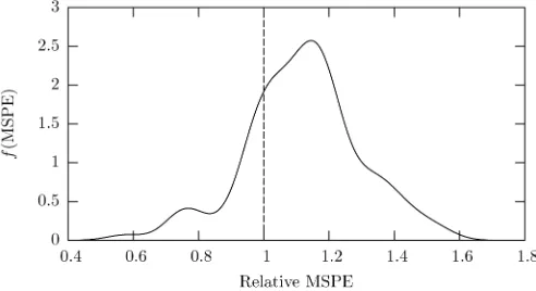
Figure 1. Density of the relative MSPE over the 100 random splits of the data. Values>1 indicate superior out-of-sample performance of the proposed method for a given random split of the data (lower quartile=1.03, median=1.13, upper quartile=1.20).
$50,000 (1970s housing prices) which makes this particularly well suited to quantile methods.
The econometric importance of this application follows from the fact that hedonic pricing models are widely used in a variety of settings; hence methods that are robust to functional specifi-cation ought to be of interest to practitioners and theoreticians alike.
We first shuffle the data and create two independent samples of sizen1=400 andn2=106. We then fit a linear parametric quantile model and a nonparametric quantile model using the estimation sample of sizen1, and generate the predicted me-dian ofYbased upon the covariates in the independent hold-out data of sizen2. Finally, we compute the mean squared predic-tion error defined as MSPE=n−21n2
i=1(Yi− ˆq.5(Xi))2, where
ˆ
q.5(Xi)is the predicted median generated from either the
para-metric or the nonparapara-metric model, andYiis the actual value of
the response in the hold-out dataset. To deflect potential crit-icism that our result reflects an unrepresentative split of the data, we repeat this process 100 times, each time computing the relative MSPE (i.e., the parametric MSPE divided by the non-parametric MSPE). For each split, we use the method of Hall et al. (2004) to compute data-dependent bandwidths. The me-dian relative MSPE over the 100 splits of the data is 1.13 (lower quartile=1.03, upper quartile=1.20), indicating that the non-parametric approach is producing superior out-of-sample quan-tile estimates. Figure 1 presents a density estimate summarizing these results for the 100 random splits of the data.
Figure 1 reveals that 76% of all sample splits (i.e., the area to the right of the vertical bar) had a relative efficiency greater than 1, or equivalently, in 76 out of 100 splits, the nonparamet-ric quantile model yields better predictions of the median hous-ing price than the parametric quantile model. Given the small sample size and the fact that there exist three covariates, we feel this is a telling application for the proposed fully nonpara-metric method. Of course, we are not suggesting that we will outperform an approximately correct parametric model. Rather, we only wish to suggest that we can often outperform com-mon parametric specifications that can be found in the litera-ture.
5. CONCLUSIONS
We propose a conditional CDF estimator defined over a mix of discrete and continuous covariates and an associated quantile function estimator. We also propose a conditional PDF-based method of data-driven bandwidth selection. In applied settings one frequently encounters a mix of datatypes; thus this esti-mator would be of value to applied researchers. Simulations demonstrate that the proposed approach performs quite well, and two applications highlight its value in applied settings. Fu-ture work includes a native method for data-driven bandwidth selection for the conditional CDF estimator.
ACKNOWLEDGMENTS
Li’s research was supported in part by the Private Enterprise Research Center, Texas A&M University. Racine would like to gratefully acknowledge support from the National Science Foundation, the Natural Sciences and Engineering Research Council of Canada (NSERC: www.nserc.ca), the Social Sci-ences and Humanities Research Council of Canada (SSHRC: www.sshrc.ca), and the Shared Hierarchical Academic Re-search Computing Network (SHARCNET:www.sharcnet.ca).
APPENDIX: PROOFS OF THEOREMS 2.1 AND 2.2
Theorem 2.1 is proved in Lemmas A.1 and A.2 below, and Theorem 2.2 is proved in Lemmas A.3 and A.4.
Lemma A.1. LetB1s(y|x)andB2s(y|x)be defined as in
The-orem 2.1. Under conditions (C1)–(C3),
E[ ˜M(y|x)] =
Therefore, (A.1) and (A.2) lead to
E[ ˜M(y|x)]
+F(y|x)2
×W(v)2dv L(zd,xd, λ)2]
+O(n−1)
=κq(nh1· · ·hq)−1[F(y|x)−F(y|x)2]
+O((nh1· · ·hq)−1(|h|2+ |λ|)+n−1). (A.4)
Lemma A.2. Under conditions (C1)–(C3),
(nh1· · ·hq)1/2
tion by Liapunov’s central limit theorem. Therefore, we have
(nh1· · ·hq)1/2[ ˜F(y|x)−F(y|x)−Bn(y|x)]
=(nh1· · ·hq)1/2A˜(y|x)/μ(x)+op(1)
→μ(x)−1N
0, μ(x)2V(y|x)
=N(0,V(y|x)) in distribution.
Lemma A.3. Under conditions (C1)–(C4),
(a) E[ ˆM(y|x)] = q
s=0h2sB1s(y|x) + rs=1λsB2s(y|x) +
o(|λ| + |h|2),
(b) V(Mˆ(y|x)) = κq(nh1· · ·hq)−1[F(y|x) − F(y|x)2 −
h0CwF0(y|x)]μ(x).
Proof. First, by Lemma A.5 we know that
E
Using an approach similar to that used to prove (A.1) and also using (A.5), we have
E[ ˆF(y|x)μ(ˆ x)]
Therefore, from (A.2) and (A.6) we obtain
E[ ˆM(y|x)]
=n−1
By Lemma A.5 we know that
E
Also, by the same calculation used in (A.4) we have
E[F(y|Xi)Kγ2(Xi,x)]
Equations (A.8) to (A.10) lead to
V(Mˆ(y|x))
=κq(nh1· · ·hq)−1μ(x)[F(y|x)−F(y|x)2−h0CwF0(y|x)]
+O(nh1· · ·hq)−1(h20+ |h|2+ |λ|)+n−1
. (A.11)
Lemma A.4. Under conditions (C1)–(C4),
(nh1· · ·hq)1/2
Proof. This follows from Lemma A.3 and the Liapunov cen-tral limit theorem (using arguments similar to those used in the proof of Lemma A.2).
Lemma A.5. Under conditions (C1)–(C4),
(a) E[G(y−Yi
We now turn to the proof of Theorem 3.1. We adopt an ap-proach similar to that of Cai (2002). We first present a lemma.
Lemma A.6. Under conditions (C1)–(C4),
ˆ
Similarly,
V[An(ǫn)]
≤n−1μ(x)−2E
G
y+ǫ
n−Yi
h0
−G
y−Y
i
h0
2
×Kγ2(Xi,x)
=O(ǫn2(nh1· · ·hq)−1).
Therefore,
ˆ
F(y+ǫn|x)− ˆF(y|x)
=An(ǫn)[1+op(1)]
=f(y|x)ǫn+Op(h20)+opǫn+(nh1· · ·hq)−1/2.
Proof of Theorem 3.1
In the proof below we will only consider the nonstochas-tic bandwidth case with h0=a00n−2/(4+q), h
s =a0sn−1/(4+q)
(s = 1, . . . ,q) and λs = b0sn−2/(4+q). By using the
tight-ness/stochastic equicontinuity argument found in Hsiao, Li, and Racine (2004), one can show that this result holds true for sto-chastic bandwidths satisfying (14).
For anyv, letǫn=Bn,α(x)+(nh1· · ·hq)−1/2Vα(x)1/2v. Then
Qα(v)
def
=P(nh1· · ·hq)1/2Vα(x)−1/2 × [ˆqα(x)−qα(x)−Bn,α(x)] ≤v
=P[ˆqα(x)≤qα(x)+ǫn]
=Pˆ
F(qα(x)+ǫn|x)≥α
=PFˆ(qα(x)|x)≥ −f(qα(x)|x)ǫn+α+o(1) (A.14)
by Lemma A.6 because h20=o((nh1· · ·hq)−1/2). Therefore,
by noting that f(qα(x)|x)Bn,α(x)=Bn(qα(x)|x), f(qα(x)|x)×
Vα(x)1/2 = V(qα(x)|x)1/2, and α = F(qα(x)|x), we have
from (A.14) that
Qn(v)= P(nh1· · ·hq)1/2Vα(x)−1/2 × [ˆqα(x)−qα(x)−Bn,α(x)] ≤v
= P
(nh1· · ·hq)1/2V(qα(x)|x)−1/2Fˆ(qα(x)|x)−α −Bn(qα(x)|x)≥ −v+o(1)
→(v),
by Theorem 2.2, where(·)is the standard normal distribution. This completes the proof.
[Received December 2004. Revised December 2005.]
REFERENCES
Aitchison, J., and Aitken, C. G. G. (1976), “Multivariate Binary Discrimination by the Kernel Method,”Biometrika, 63, 413–420.
Bierens, H. (1987), “Kernel Estimators of Regression Functions,” inAdvances in Econometrics: Fifth World Congress, Vol. I, ed. T. Bewley, New York: Cambridge University Press, pp. 99–144.
Buchinsky, M. (1994), “Changes in the U.S. Wage Structure 1963–1987: Ap-plication of Quantile Regression,”Econometrica, 62, 405–458.
Buchinsky, M., and Hahn, J. (1998), “An Alternative Estimator for the Censored Quantile Regression Model,”Econometrica, 66, 653–671.
Cai, Z. (2002), “Regression Quantiles for Time Series Data,”Econometric The-ory, 18, 169–192.
Cai, Z., and Xu, X. (2004), “Nonparametric Quantile Estimations for Dynamic Smooth Coefficient Models,” technical report, University of North Carolina, Dept. of Mathematics and Statistics.
Chaudhuri, P. (1991), “Nonparametric Estimates of Regression Quantiles and Their Local Bahadur Representation,”The Annals of Statistics, 19, 760–777. Chaudhuri, P., Doksum, K., and Samarov, A. (1997), “On Average Derivative
Quantile Regression,”The Annals of Statistics, 25, 715–744.
Guerre, E., Perrigne, I., and Vuong, Q. (2000), “Optimal Nonparametric Esti-mation of First-Price Auctions,”Econometrica, 68, 525–574.
Hall, P., Racine, J., and Li, Q. (2004), “Cross-Validation and the Estimation of Conditional Probability Densities,”Journal of the American Statistical Association, 99, 1015–1026.
Hall, P., Wolff, R. C. L., and Yao, Q. (1999), “Methods for Estimating a Con-ditional Distribution Function,”Journal of the American Statistical Associa-tion, 94, 154–163.
Hansen, B. (2004), “Nonparametric Estimation of Smooth Conditional Distrib-utions,” technical report, University of Wisconsin.
He, X., and Ng, P. (1999), “Quantile Splines With Several Covariates,”Journal of Statistical Planning and Inference, 75, 343–352.
He, X., Ng, P., and Portony, S. (1998), “Bivariate Quantile Smoothing Splines,”
Journal of the Royal Statistical Society, Ser. B, 60, 537–550.
Honda, T. (2000), “Nonparametric Estimation of a Conditional Quantile for
α-Mixing Processes,”Annals of the Institute of Statistical Mathematics, 52, 459–470.
Horowitz, J. (1998), “Bootstrap Methods for Median Regression Models,”
Econometrica, 66, 1327–1352.
Hsiao, C., Li, Q., and Racine, J. (2004), “A Consistent Model Specification Test With Mixed Categorical and Continuous Data,” unpublished manuscript, Texas A&M University, Dept. of Economics.
Jones, M., and Hall, P. (1990), “Mean Squared Error Properties of Kernel Estimates of Regression Quantiles,”Statistics and Probability Letters, 10, 283–289.
Koenker, R. (2004),quantreg: Quantile Regression, R package version 3.72, Initial R port from Splus by Brian Ripley (ripley@stats.ox.ac.uk). Koenker, R., and Bassett, G. (1978), “Regression Quantiles,”Econometrica, 46,
33–50.
Koenker, R., and Xiao, Z. (2002), “Inference on the Quantile Regression Process,”Econometrica, 70, 1583–1612.
(2004), “Unit Root Quantile Autoregression Inference,”Journal of the American Statistical Association, 99, 775–787.
Li, Q., and Racine, J. (2003), “Nonparametric Estimation of Distributions With Categorical and Continuous Data,”Journal of Multivariate Analysis, 86, 266–292.
Li, T., Perrigne, I., and Vuong, Q. (2000), “Conditional Independent Private In-formation in OCS Wildcat Auctions,”Journal of Econometrics, 98, 131–161. Matzkin, R. L. (2003), “Nonparametric Estimation of Nonadditive Random
Functions,”Econometrica, 71, 1339–1375.
Powell, J. L. (1986), “Censored Regression Quantiles,”Journal of Economet-rics, 32, 143–155.
Racine, J., and Li, Q. (2004), “Nonparametric Estimation of Regression Func-tions With Both Categorical and Continuous Data,”Journal of Econometrics, 119, 99–130.
Tsay, R. S. (2002),Analysis of Financial Time Series, New York: Wiley. Yu, K., and Jones, M. C. (1998), “Local Linear Quantile Regression,”Journal
of the American Statistical Association, 93, 228–237.