Full Terms & Conditions of access and use can be found at
http://www.tandfonline.com/action/journalInformation?journalCode=ubes20
Download by: [Universitas Maritim Raja Ali Haji] Date: 12 January 2016, At: 23:27
ISSN: 0735-0015 (Print) 1537-2707 (Online) Journal homepage: http://www.tandfonline.com/loi/ubes20
Comment
René Garcia & Nour Meddahi
To cite this article: René Garcia & Nour Meddahi (2006) Comment, Journal of Business &
Economic Statistics, 24:2, 184-192, DOI: 10.1198/073500106000000161
To link to this article: http://dx.doi.org/10.1198/073500106000000161
Published online: 01 Jan 2012.
Submit your article to this journal
Article views: 42
Comment
René G
ARCIADépartement de Sciences Économiques, CIRANO, CIREQ, Université de Montréal, Montréal, Québec, H3C 3J7, Canada (rene.garcia@umontreal.ca)
Nour M
EDDAHIDépartement de Sciences Économiques, CIRANO, CIREQ, Université de Montréal, Montréal, Québec, H3C 3J7, Canada (nour.meddahi@umontreal.ca)
1. A HISTORICAL REVIEW
The authors are to be congratulated for an excellent contri-bution, from both a theoretical and an applied standpoint, to the problem of measuring integrated variance in the presence of microstructure noise, an inescapable reality.
The negative effects of microstructure noise on measuring volatility have been well known for years. For instance, French, Schwert, and Stambaugh (1987) incorporated the cross-product of consecutive days to take into account the first-order auto-correlation of daily returns caused by nonsynchronous trading of securities. Note that the estimator proposed by French et al. (1987) coincides with the one proposed by Zhou (1996) and an-alyzed by Hansen and Lunde (HL). Of course, we know from the current literature (e.g., Zhang, Mykland, and Aït-Sahalia 2004; Bandi and Russell 2005a; Hansen and Lunde 2005a,b, 2006) that microstructure noise plays a crucial role in measur-ing daily integrated variance, but less so in measurmeasur-ing monthly integrated variance. This gives a theoretical foundation to the work of French et al. (1987), who found that the correction is not that important quantitatively.
Microstructure noise was also a well-known problem at the inception of the current literature. Fifteen years ago, Daniel Nelson (1958–1995) was among the pioneers who established the theoretical foundations for measuring instantaneous vari-ance from high-frequency data. Bollerslev and Rossi (1995) reviewed his numerous contributions, particularly that on mea-suring, filtering, and forecasting variance. Daniel Nelson’s research agenda, combined with the availability of high-frequency data (provided by, most notably, the Olsen group), lead several authors, particularly Torben Andersen and Tim Bollerslev, to explore empirically the issue of nonparametric measurement of instantaneous variance. They obviously ran into the problem of microstructure effects, especially the in-traday periodicity (see, e.g., Andersen and Bollerslev 1997). At the same time, another research strand was developed un-der the leaun-dership of Robert Engle with the goal of extracting the information on volatility contained in the durations between consecutive trades (see, e.g., Engle 2000).
Closer to the current literature, an important breakthrough can be attributed to Andersen and Bollerslev (1998), as well as Barndorff-Nielsen and Shephard (2001). For instance, Andersen and Bollerslev (1998) clearly showed the importance of measuring daily integrated variance by summing squared intradaily returns. Moving from measuring instantaneous vari-ance to integrated varivari-ance was theoretically successful due to the availability of a central limit theorem (Jacod and Protter 1998; Barndorff-Nielsen and Shephard 2002). This move was
also empirically successful because intraday periodicity plays a less important role. Moving from instantaneous to integrated variance is indeed a temporal aggregation issue, and it is well known from the macroeconometric literature that aggregat-ing helps solve the seasonality problem. The empirical suc-cess of this approach was clearly demonstrated by Andersen, Bollerslev, Diebold, and Labys (2001, 2003).
We finish this section with some historical notes. Andersen and Bollerslev (1997) gave a presentation at the World Congress of the Econometric Society in Tokyo (1995). At the same congress, Éric Renault gave an invited lecture on financial econometrics and ended his talk by saying that the financial econometrics lecture at the next World Congress should focus on the problems related to microstructure effects (see Renault 1997). In fact, it took 10 years to have lectures on the topic, by Yacine Aït-Sahalia and Neil Shephard, at the last World Congress in London. Engle (2000) gave the Fisher–Schultz in-vited lecture of the European meeting of the Econometric Soci-ety in Istanbul in 1996. Also note that at the end of Aït-Sahalia and Shephard’s talks, Engle made the comment that the iid as-sumption of noise clearly is not empirically supported by the data, because durations (i.e., the time between two consecutive trades) contain information on volatility.
The rest of this comment is organized as follows. Section 2 discusses several issues about statistical inference when one faces microstructure noise. Section 3 studies the time series properties of the realized variance under the presence of mi-crostructure noise. The last section discusses the economic im-portance of accounting and correcting for microstructure noise and identifies the questions for which it may be relevant to do so.
2. MICROSTRUCTURE NOISE AND STATISTICAL INFERENCE
2.1 The Signature Plot
HL’s article is one of several works in the current litera-ture devoted to establishing the statistical properties of estima-tors under maintained assumptions about microstructure noise, mainly iid or serially correlated noise. One important tool for analyzing these estimators is the signature plot. However, these assumptions are not explicitly tested. HL use the behavior of the
© 2006 American Statistical Association Journal of Business & Economic Statistics April 2006, Vol. 24, No. 2 DOI 10.1198/073500106000000161
signature plots of various realized variance estimators to infer the properties of the noise, with a flat signature plot being con-sistent with the absence of noise. This approach is very useful and informative, but it does not constitute a formal test.
To show the limitations of the signature plot as an inference tool, we consider a particular example where expressions can be computed in closed form. We propose a model where the microstructure noise is stationary. Then we show that for some specific values of the parameters, one can have a signature plot of realized variance that looks like one corresponding to the iid microstructure noise case. Again, this example is provided to show that the current literature neglects to formally test the assumptions made on the microstructure noise and instead uses “visual” diagnostics.
Assume that the noise processutis stationary and given by
ut=
t
−∞
A(t−u)dWu, (1)
whereWuis a standard Brownian process, independent of the
efficient price process p∗t, and A(·) is a real function such that ∞
0 A2(u)du<∞. Observe that the Ornstein–Uhlenbeck (OU) process considered by Aït-Sahalia, Mykland, and Zhang (2005a), that is,
dut= −κutdt+σdWt,
corresponds to the case where
A(s)=σexp(−κs).
Feunou, Garcia, Meddahi, and Tedongap (2005) showed that
E[RVt(h)] =E[RV∗t(h)] +h−1E
whereπ(·)is defined in HL’s assumption 2. Consequently, there is a connection betweenA(·)andπ(·). For instance, one can show that the daily quadratic variation of the processutequals A2(0)and, therefore,A2(0)= −2π′(0).
Instead of considering the OU process, in what follows we assume a more general process given by
A(s)= formulas of (6), (7), and (8), in the Appendix.
Our main goal in the rest of this section is to consider several values forθ=(κ1, κ2,s0)to study the behavior of
that is, the difference between the ideal signature plot (no mi-crostructure noise) and the observed one (with mimi-crostructure noise). Given that there is a scaling issue, instead of studying the functionf(·), we study the functiong(·)defined by
In other words, we assume a unit variance for the noise ut.
Moreover, the unit of time is not specified. As usual, the non-invariant measure is κt; that is, by varying the parameters κ andtand maintaining the productκtfixed, we get the same results, which we show later.
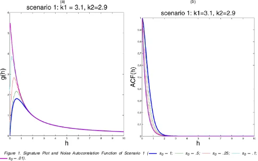
The first scenario that we consider is (κ1, κ2)=(3.1,2.9), with s0 taking several values {.01, .1, .25, .5,1}. Figure 1(a) plotsg(·), and Figure 1(b) provides the ACF of the microstruc-ture noiseut. If we defineh∗as the argmax ofg(·), then the right
part of Figure 1(a) (i.e.,h>h∗) looks like the realized variance signature plot. Note that in practice,s0may be very small, and thus we cannot observe the left part of the function g(·), that is, we cannot distinguish the noise considered here from an iid one.
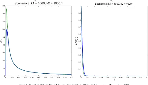
Of course, we could argue that the magnitude of the maxi-mum is not important, especially for a unit variance noise. Ac-tually, we can readily increase this maximum by raising the values of κ1 and κ2 and lowering the value of s0. We con-sider two other scenarios: (κ1, κ2)=(500,500.1) with s0∈
{.001, .01} (scenario 2) and (κ1, κ2)=(1,000,1,000.1) with s0∈ {.001, .01}(scenario 3). Figures 2(a) and 3(a) plot the func-tiong(·), where clearly the maximums are now very high.
Figures 1(b), 2(b), and 3(b) plot the autocorrelation functions of the microstructure noise in the three scenarios. Given that we take large values for κ1 andκ2, the autocorrelations van-ish quickly to 0 (especially for the second and third scenarios), meaning that the noise is almost iid but with finite variation. Again, this feature will increase the problem of identification.
We end this section with two remarks:
1. In these examples we focused on small values ofhgiven that the quadratic variation of the microstructure noise equalsA(0). However, for a given sample frequency, the behavior ofA(h)for h=0 plays a role in the signature plot.
2. One could argue that the examples provided here do not match the signature plot for different values of the sample frequency. A simple approach to handle this problem is to add a dependent noise (e.g., OU) to our examples to match the signature plot beyond the origin.
(a) (b)
Figure 1. Signature Plot and Noise Autocorrelation Function of Scenario 1 ( s0=1; s0=.5; s0=.25; s0=.1; s0=.01).
(a) (b)
Figure 2. Signature Plot and Noise Autocorrelation Function of Scenario 2 ( s0=.01; s0=.001).
(a) (b)
Figure 3. Signature Plot and Noise Autocorrelation Function of Scenario 3 ( s0=.01; s0=.001).
2.2 Nonnegative Estimators
One desirable property of any estimator of the integrated variance is nonnegativity. There is no reason to believe that the current estimator or those estimators that correct the bias are nonnegative. Of course, one could use more adequate kernels (e.g., the Bartlett kernel) to ensure positivity, as in the HAC lit-erature (Newey and West 1987; Andrews 1991). But it is not clear whether one can find such a kernel and obtain an optimal estimator of the integrated variance as was done by Barndorff-Nielsen, Hansen, Lunde, and Shephard (2004) (which is closely related to the optimal subsample estimator in Zhang 2004).
Some authors have considered the multivariate case, in par-ticular, Bandi and Russell (2005b) and Hayashi and Yoshida (2005). However, these authors focused on estimating the covariance and the variances independently, that is, without imposing the Cauchy–Schwarz inequality, which leads to the possibility of having variance–covariance estimators that are not nonnegative. Again, an approach based on kernel may be helpful in solving this problem (but will still face the problem of nonsynchronous trades).
A different approach would be first to prewhiten or filter the data, as was done by Ebens (1999) and Andersen et al. (2001), and then to compute the usual realized variance of the trans-formed data, thereby obtaining nonnegative estimators. Under some assumptions, Bandi and Russell (2005a) studied the the-oretical properties of such estimators and reached somewhat mixed conclusions. We believe, however, that this approach de-serves more study because it is simple and provides nonnegative estimators (in both the univariate and the multivariate cases). A more fundamental argument was provided by Smith (2005), who drew a theoretical connection between the HAC estimators
and estimators computed as the variance of transformed data. Although these transformations are motivated by the literature on empirical likelihood, they can be interpreted as prewhitening or filtering methods.
2.3 Calendar or Transaction Time Sampling
As emphasized by Hasbrouck (2006), microstructure time se-ries are distinctive because market data are discrete events re-alized in continuous time (so-called point processes) and are well ordered. Macroeconomic time series are typically time-aggregated and become positively correlated by construction. In contrast, tick-by-tick data are well ordered in time.
For the issue at hand in Hansen and Lunde’s article—the in-fluence of microstructure noise on the estimation of model-free realized variance—the distinction between transaction or quo-tation prices and “artificial” prices constructed from an equidis-tant calendar time sampling is certainly of central interest. This is important with respect to both the bias introduced by in-creased sampling frequency in the measure of realized variance and its influence on bias correction by a kernel-type estimator.
Oomen (2005) modeled the efficient martingale component of the observed price as a compound Poisson process. In this setting, expressions for the bias and the mean squared er-ror (MSE) of the bias-corrected realized variance (through the same Newey–West procedure as in this article) are available in closed form. He showed that the bias correction allows one to considerably increase the optimal sampling frequency and pro-duce a sizeable reduction in MSE of the realized variance. This is comparable to the results presented in this article. More inter-estingly, however, transaction time sampling delivers a superior measure relative to calendar time sampling. The fact that the
price process is sampled in transaction time reduces the MSE by about 20%. This is not apparent in the results of this arti-cle. Oomen attributed the error reduction mainly to the fact that returns sampled in transaction time are devolatized through an appropriate deformation of the time scale. In transaction time sampling, the time scale is deformed by the expected and the realized number of transactions. This suggests an adjustment to the procedure for the computation of realized variance with cal-endar time sampling. Indeed, the main information missing in calendar time sampling is the level of activity in the market, and thus the quantity of information potentially incorporated in the efficient price. Instead of weighting each time interval equally, one can consider weighting the time intervals by the number of transactions occurring during the intervals. This idea could serve also to construct a noise-to-signal ratio,λ, that could vary from day-to-day according to the level of activity in the market. We end this section with one remark about HL’s lemma 1. This lemma suggests that one should avoid the linear interpo-lation method. Maybe this is a good advice, but we find that lemma 1 does not provide a theoretical foundation for such a recommendation. The critical point in the proof of lemma 1 is the assumption onN, the number of trades, which is assumed constant. This assumption is quite peculiar. For instance, one should ask the same question: What is the limit of RV(m) as
m→ ∞ if one uses the previous-tick method and maintains
Nconstant? It is certainly not the quadratic variation!
2.4 Durations
As noted in Section 1 of our comment, the durations (i.e., times between consecutive trades) contain information about the volatility. This was clearly established by Engle (2000). Consequently, extracting this information is of interest. Of course, it might be difficult to do this in a nonparametric setting but even results in a parametric world will aid understanding of the interaction between volatility and the transaction process. Some preliminary and interesting results have been provided by Renault and Werker (2004) in a semiparametric world clearly showing that a causality between the durations and the variance has an impact on the characteristics of integrated variance, par-ticularly its expectation (and thus its forecast).
2.5 The Loss Function
HL’s article, as well as several papers in the literature, fo-cuses on the MSE of the realized variance measures. However, in several economic examples, the object of interest is not the variance, but rather a nonlinear function of it. For instance, in the context of optimal portfolio analysis, the object of interest is the inverse of the volatility. Of course, when one has a con-sistent estimator and a central limit theorem, the delta method allows the study of any nonlinear function of the variance.
2.6 Estimation of the Optimal Frequency
Here we focus on the empirical application of corollary 2, in particular estimation of the optimal frequency for an estima-tor of the integrated variance (e.g., RV(m) or RV(ACm)
1). As HL
point out in their article, an approximation of the optimal fre-quency for the estimatorRV(ACm)
ω2is the variance of the processut. Consequently, the optimal
length of returns is2√ω2
3 1
IV. Two main remarks are in order. First,
given that the integrated variance is time-varying, the optimal length/frequency of observations is time-varying. Second, the optimal length/frequency is a function of the object of inter-est, that is, the integrated variance; therefore, estimating this length/frequency is difficult.
The current literature follows two approaches to handling this problem. The first approach involves estimating the daily integrated variance at a lower frequency where microstructure noise is small. However, at such frequencies, the discretiza-tion noise is quite important (see, e.g., Barndorff-Nielsen and Shephard 2002; Meddahi 2002; Gonçalves and Meddahi 2005). The second approach involves estimating the empirical mean of the realized variance (computed again at a low frequency) over several days. In other words, this approach ignores the time variation in the integrated variance. In so doing, it neglects the effect of Jensen’s inequality. The daily optimal length is propor-tional toIV−1and not toIV. Therefore, there is a bias. Actually, given that the functionf(x)=x−1is convex forx>0, one will
underestimatethe optimal length of returns. A similar analysis may be done for the other measures.
In a Monte Carlo experiment, we quantify the magnitude of the bias. We consider two models with no drift and leverage effect from Bollerslev and Zhou (2002),
dp∗t =σtdWt, dσt2=.03(.25−σt2)dt+.1σtdW1,t,
and
dp∗t =σtdWt, σt2=σ12,t+σ22,t,
dσ12,t=.5708(.3257−σ12,t)dt+.2286σ1,tdW1,t, dσ22,t=.0757(.1786−σ22,t)dt+.1096σ2,tdW2,t.
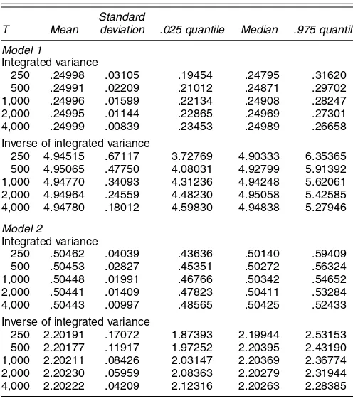
The results, based on 5,000, replications are reported in Ta-ble 1. The taTa-ble provides the mean, the standard deviation, and some quantiles ofIVt andIV−t 1. There is a clear and nonneg-ligible Jensen’s effect. For instance, considering model 2, esti-mated by Bollerslev and Zhou (2002) on DM/$ exchange rates for the sample period December 1, 1986–December 1, 1996, (E[IVt])−1equals 1.98 andE[IV−t 1]equals 2.20.
2.7 Cointegration
A way to improve the quality of the efficient price compo-nent is to use several prices—transaction, ask or bid quote, and mid-quote—to extract the efficient price and noise. Hansen and Lunde propose using a cointegration method to decompose the prices into a common stochastic trend and transitory compo-nents, enabling evaluation of the contributions of innovations in the various price series to the efficient price series. The results confirm the importance of the information content in transac-tion prices, at least for the securities on the New York Stock Exchange (a specialist market), because larger instantaneous correlations between the transaction price and the efficient price are observed.
The methodology used by Hansen and Lunde is based on that of Hasbrouck (1995), who used prices of the same security on several exchanges to better estimate the efficient price. Another
Table 1. Characteristics of IVtand IV−t
Standard
T Mean deviation .025 quantile Median .975 quantile
Model 1
Integrated variance
250 .24998 .03105 .19454 .24795 .31620
500 .24991 .02209 .21012 .24871 .29702
1,000 .24996 .01599 .22134 .24908 .28247
2,000 .24995 .01144 .22865 .24969 .27301
4,000 .24999 .00839 .23453 .24989 .26658
Inverse of integrated variance
250 4.94515 .67117 3.72769 4.90333 6.35365 500 4.95065 .47750 4.08031 4.92799 5.91392 1,000 4.94770 .34093 4.31236 4.94248 5.62061 2,000 4.94964 .24559 4.48230 4.95058 5.42585 4,000 4.94780 .18012 4.59830 4.94838 5.27946
Model 2
Integrated variance
250 .50462 .04039 .43636 .50140 .59409
500 .50453 .02827 .45351 .50272 .56324
1,000 .50448 .01991 .46766 .50342 .54652
2,000 .50441 .01409 .47823 .50411 .53284
4,000 .50443 .00997 .48565 .50425 .52433
Inverse of integrated variance
250 2.20191 .17072 1.87393 2.19944 2.53153 500 2.20177 .11917 1.97252 2.20395 2.43190 1,000 2.20211 .08426 2.03147 2.20369 2.36774 2,000 2.20230 .05959 2.08363 2.20279 2.31944 4,000 2.20222 .04209 2.12316 2.20263 2.28385
way to improve the quality of the efficient price component is to use information on several securities through correlations be-tween the efficient prices or the microstructure noises. A mul-tivariate analysis of efficient prices and noises raises at least two issues: synchronization and specification of the variance– covariance matrices. Bandi and Russell (2005c) avoided the first problem by constructing equal-spaced continuously com-pounded returns using mid-quotes and the previous tick method (see Hayashi and Yoshida 2005 for a different approach). More-over, Bandi and Russell (2005c) made simplifying assumptions about the correlations over time and across securities. One im-portant characteristic of the covariance matrix is that it should be semidefinite positive. As we pointed out in Section 2.2, the estimator of Bandi and Russell (2005c) does not impose this property by construction.
Also, as pointed out earlier for a different issue, there are some identification problems when one wants to disentangle the efficient price from the noise. Assumptions are needed. The as-sumptions made in the cointegration part are not clear, at least to us. More details may be helpful.
3. TIME SERIES PROPERTIES OF REALIZED VARIANCE UNDER MICROSTRUCTURE NOISE
3.1 Dynamics of the Realized Variance Under Microstructure Noise
Barndorff-Nielsen and Shephard (2002) and Meddahi (2003) studied the time series properties of the realized variance when there is no microstructure noise. More precisely, these au-thors derived the state-space and autoregressive moving aver-age (ARMA) representations of the realized variance when the process of the instantaneous variance is specified as a linear
combination of autoregressive processes. We now study these representations under the presence of microstructure noise.
For simplicity, we assume that the microstructure noise,ut, is
iid; the rest of this section provides results given by Andersen, Bollerslev, and Meddahi (2005), who showed the following.
Proposition 1. Let Jt ≡σ (pτ,fτ,uτ, τ ≤t, τ ∈ ℜ) where
fτ is the Markov state variable that drives the volatility process
σt, then
In this section we focus on the ARMA representation of the realized variance. Equation (13) implies that the covariance of the true realized variance and the observed one have quite sim-ilar ARMA representations in the settings of Barndorff-Nielsen and Shephard (2002) and Meddahi (2003); the orders of the ARMA are the same, as are the autoregressive roots. However, there is a difference in the moving average roots, as well as between the unconditional means [which is equal to 2Vuh−1;
see (10)]. There is also an important difference between the variance of the two variables. In addition, the variance of the noisy realized variance goes to infinity whenh→0 given that the quadratic variation of the noise is unbounded [see (11)]. This suggests that the autocorrelation function of the noisy re-alized variance will vanish to 0 whenh→0.
Table 2 provides these autocorrelation functions for the DM/$ spot rates used by Andersen, Bollerslev, and Diebold
Table 2. Autocorrelation Function of the DM/$ Realized Variance
1/h
lag 288 144 48 24
1 .5501 .4764 .3760 .3392
2 .4284 .3835 .3136 .2907
3 .3573 .3128 .2451 .2306
4 .3387 .3147 .2361 .2231
5 .3330 .2935 .2078 .1878
10 .2740 .2395 .1709 .1512
15 .2478 .2193 .1821 .1581
20 .1785 .1645 .1305 .0985
30 .1167 .1114 .0759 .0564
40 .0986 .0910 .0717 .0731
50 .0842 .0758 .0552 .0596
(2005). The results on the S&P500 and the U.S. Treasury Bond futures are similar and are not reported. For the DM/$,h=288 corresponds to 5 minutes, h=144 to 10 minutes, and so on. Even though we are not providing a formal test, a look at Ta-ble 2 suggests that the iid assumption of the microstructure noise is not supported by the data. In particular, it is not at all clear that the autocorrelation function goes to 0 whenh→0. Actually, for a given lag, the autocorrelation increases when
h decreases; that is, as in the nonmicrostructure case, the per-sistence of the instantaneous variance dominates when h de-creases.
The calculations that we have derived here can be extended to the non-iid case. In particular, it is clear that the dynamics of the noisy realized variance contains information about the dynamics of the microstructure noise. It will be interesting to explore this avenue in future research.
3.2 Forecasting Integrated Variance Based on Realized Variance Under Microstructure Noise
Andersen, Bollerslev, and Meddahi (2004) gave an analytical explanation for the empirical finding of Andersen, Bollerslev, Diebold, and Labys (2003) that realized variance can be well forecasted. The work of Andersen, Bollerslev, and Meddahi (2004) was based on analytical formulas for the autocovari-ance functions of the realized variautocovari-ance under nonmicrostruc-ture noise when one assumes that the data-generating process is the eigenfunction stochastic volatility model of Meddahi (2001). Proposition 1 allows extension of the work of Andersen, Bollerslev, and Meddahi (2005) to the presence of microstruc-ture noise.
As shown in Proposition 1, the noisy realized variance is less predictable than the realized variance. In addition, the em-pirical autocorrelation functions of the noisy realized variance are clearly high. Therefore, the predictability of realized vari-ance and integrated varivari-ance is higher than that suggested by Andersen, Bollerslev, Diebold, and Labys (2003). Of course, some problems must be fixed. For instance, the forecast is bi-ased given that the means of the noisy realized variance and realized variance are different. Again, a simple approach to fix this problem is to adjust the mean.
Of course, there are several estimators of the integrated vari-ance under microstructure noise, including those that mini-mize the MSE of the estimator and those that are consistent. Andersen, Bollerslev, and Meddahi (2005) also studied their forecasting power; in particular, results like those in Proposi-tion 1 will be derived for these estimators for iid noise as well as stationary and serially correlated noise.
3.3 Estimation of Continuous Time Stochastic Volatility Models Based on Realized Variance Under Microstructure Noise
Barndorff-Nielsen and Shephard (2002) and Bollerslev and Zhou (2002) estimated continuous-time models using daily re-alized variance. Barndorff-Nielsen and Shephard (2002) used the state-space representation of the realized variance and esti-mated the model by using the quasi-maximum likelihood com-bined with the Kalman filter. In contrast, Bollerslev and Zhou
(2002) derived some moments fulfilled by the integrated vari-ance assuming a square root process for the varivari-ance, then used an instrumental variables method to estimate the parameters by using the realized variance data instead of the unobservable in-tegrated variance data.
Corradi and Distaso (2004) extended the work of Bollerslev and Zhou (2002) to the eigenfunctions stochastic volatility model of Meddahi (2001). In addition, Corradi and Distaso (2004) gave a theoretical foundation for the approach that ignores the difference between the integrated variance and con-sistent realized measures like the two-scale estimator of Zhang, Mykland, and Aït-Sahalia (2005).
Feunou et al. (2005) have explored in detail the impact of microstructure noise on estimating continuous-time models (by the Kalman filter, as in Barndorff-Nielsen and Shephard 2002 and by generalized method of moments as in Bollerslev and Zhou 2002). We obviously find an impact (albeit a not very im-portant one) that can be easily explained. We showed earlier that microstructure noise implies that the noisy realized vari-ance has the same autoregressive part as the nonnoisy one, but with a different unconditional mean and moving average part. The autoregressive part identifies the mean reverting parameters and thus is not sensitive to the microstructure noise. The un-conditional mean can be easily adjusted. The moving average part of the noisy realized variance is a function of the mean-reverting parameters, the unconditional mean, and the variance of the variance parameters. Consequently, the variance of the variance is overestimated. However, the variance of the vari-ance is not well estimated even in the absence of microstructure noise (see Barndorff-Nielsen and Shephard 2002; Bollerslev and Zhou 2002).
4. THE ECONOMIC IMPORTANCE OF MICROSTRUCTURE NOISE
An important motivation invoked by Bandi and Russell (2005c) for multivariate analysis is the portfolio allocation problem. This raises the issue of the economic significance of optimally sampling the returns at higher frequencies than, say, the 5-minute or 15-minute sampling typically used in the literature. This is a central issue that HL do not analyze. They use the methodology of Fleming, Kirby, and Ostdiek (2001, 2003) to measure the fees that an investor would be willing to pay to switch from a covariance forecast based on 5-minute or 15-minute sampling to optimally sampled realized covariances. They consider an investor who uses a conditional mean-variance optimization rule to allocate funds in several classes of assets with daily rebalancing. Given a mean return target, the gains in variance reduction will be translated into an economic quantity by simply scaling them by a risk aver-sion factor. One needs a high risk averaver-sion parameter and a high mean return target to arrive at economic significant fees (at most 67 basis points per year, with a mean target of 15% and an absolute risk aversion of 10).
Another economic application for realized variance has been the extraction of a volatility risk premium, as proposed by Garcia, Lewis, and Renault (2001). This methodology is based on estimating jointly the objective and risk-neutral parame-ters of stochastic volatility diffusion models. This procedure is
based on series expansions of option prices and implied volatil-ities and on a method-of-moments estimation that uses ana-lytical expressions for the moments of the integrated variance and realized variance measures. Recently, Bollerslev, Gibson, and Zhou (2004) followed a similar course with nonparamet-ric measures of implied volatility instead of series expansions. Once these parameters are estimated, one can imagine an appli-cation of the stochastic volatility model to, say, pricing options and measure the economic impact of using various frequen-cies for computing realized variance. However, the frequency at which these applications are conducted is typically 1 month, because interest lies in comparing the dynamics of the risk pre-mium with several macroeconomic variables. Therefore, the statistical refinements developed by Hansen and Lunde cannot be considered very useful for these types of applications.
The potential economic importance of the statistical refine-ments proposed by Hansen and Lunde and others should be gauged in market microstructure models. Hasbrouck (2006) provided a list of important questions in market microstruc-ture, including the incorporation of information in prices, the relationship between market structure and the valuation of se-curities, and the mechanisms to better aggregate information into prices. In these models, it is often the case that sampling is determined by information arrivals. Recently, Owens and Steigerwald (2005) developed a microstructure model to es-timate the frequency and quality of private information. The frequency of private information is measured by the potential revelation of the information at each arrival. In our view, it is more important that the potential gains associated with high-frequency sampling and with bias corrections be assessed in these settings.
ACKNOWLEDGMENTS
This work was supported by grants from FQRSC, Hydro-Quebéc, MITACS, and SSHRCC. In addition, René Garcia thanks Bank of Canada, and Nour Meddahi thanks Jean-Marie Dufour’s Econometrics Chair of Canada and CREST for their financial support. The authors thank Bruno Feunou and Roméo Tedongap for excellent research assistance, and Silvia Gonçalves for helpful discussions.
APPENDIX: FORMULAS OF (6), (7), AND (8) FOR THE GENERAL EXAMPLE OF SECTION 2.1
We can show the following:
• Ifh≤s0, then
• In addition, we have
var(ut)=
Andersen, T. G., Bollerslev, T., and Diebold, F. X. (2005), “Roughing It Up: Including Jump Components in the Measurement, Modeling and Forecast-ing of Return Volatility,” workForecast-ing paper, Northwestern University, Dept. of Finance.
Andersen, T. G., Bollerslev, T., Diebold, F. X., and Labys, P. (2001), “The Dis-tribution of Realized Exchange Rate Volatility,”Journal of the American Sta-tistical Association, 96, 42–55.
Andersen, T. G., Bollerslev, T., and Meddahi, N. (2005), “Market Microstruc-ture Noise and Realized Volatility Forecasting,” unpublished manuscript, Université de Montréal, Dept. of Economics.
Bandi, F., and Russell, J. (2005a), “Microstructure Noise, Realized Volatility, and Optimal Sampling,” working paper, University of Chicago, Graduate School of Business.
(2005b), “Realized Covariation, Realized Beta, and Microstructure Noise,” working paper, University of Chicago, Graduate School of Business. (2005c), “Separating Microstructure Noise From Volatility,”Journal of Financial Economics, forthcoming.
Barndorff-Nielsen, O. E., and Shephard, N. (2001), “Non-Gaussian Ornstein– Uhlenbeck–Based Models and Some of Their Uses in Financial Economics,” Journal of the Royal Statistical Society, Ser. B, 63, 167–241.
Bollerslev, T., Gibson, M., and Zhou, H. (2004), “Dynamic Estimation of Volatility Risk Premia and Investor Risk Aversion From Option-Implied and Realized Volatilities,” discussion paper, Federal Reserve Board.
Bollerslev, T., and Rossi, P. E. (1995), “Dan Nelson Remembered,”Journal of Business & Economic Statistics, 13, 361–364.
Bollerslev, T., and Zhou, H. (2002), “Estimating Stochastic Volatility Diffusion Using Conditional Moments of Integrated Volatility,”Journal of Economet-rics, 109, 33–65.
Corradi, V., and Distaso, W. (2004), “Estimating and Testing Stochastic Volatil-ity Models Using Realized Measures,” working paper, Queen Mary, Univer-sity of London.
Engle, R. F. (2000), “The Econometrics of Ultra-High–Frequency Data,” Econometrica, 68, 1–22.
Feunou, B., Garcia, R., Meddahi, N., and Tedongap, R. (2005), “Estimation of Continuous-Time Models Based on Realized Measures: A Comparison of Methods,” unpublished manuscript, Université de Montréal, Dept. of Eco-nomics.
Fleming, J., Kirby, C., and Ostdiek, B. (2001), “The Economic Value of Volatil-ity Timing,”Journal of Finance, 56, 329–352.
(2003), “The Economic Value of Volatility Timing Using ‘Realized’ Volatility,”Journal of Financial Economics, 67, 473–509.
Garcia, R., Lewis, M.-A., and Renault, E. (2001), “Estimation of Objective and Risk-Neutral Distributions Based on Moments of Integrated Volatility,” working paper, Université de Montréal, Dept. of Economics, and CIRANO. Hasbrouck, J. (2006),Empirical Market Microstructure, Oxford University
Press, in press.
Hayashi, T., and Yoshida, N. (2005), “On Covariance Estimation of Nonsyn-chronously Observed Diffusion Processes,”Bernoulli, 11, 359–379. Meddahi, N. (2001), “An Eigenfunction Approach for Volatility Modeling,”
working paper, Université de Montréal, Dept. of Economics.
(2003), “ARMA Representation of Integrated and Realized Variances,” The Econometrics Journal, 6, 334–355.
Owens, J., and Steigerwald, D. G. (2005), “Inferring Information Frequency and Quality,”Journal of Financial Econometrics, 3, 500–524.
Renault, E. (1997), “Econometric Methods of Option Pricing Errors,” in Advances in Economics and Econometrics: Theory and Applications, 7th WCES, Vol. 3, eds. D. M. Kreps and K. F. Wallis, Cambridge, U.K.: Cambridge University Press, pp. 223–278.
Renault, E., and Werker, B. J. M. (2004), “Stochastic Volatility Models With Transaction Time Risk,” working paper, Tilburg University, Dept. of Eco-nomics.
Smith, R. (2005), “Automatic Positive Semidefinite HAC Covariance Matrix and GMM Estimation,”Econometric Theory, 21, 158–170.
Comment
Eric G
HYSELSDepartment of Finance, Kenan-Flagler School of Business, and Department of Economics, University of North Carolina, Chapel Hill, NC 27599-3305 (eghysels@unc.edu)
Arthur S
INKODepartment of Economics, University of North Carolina, Chapel Hill, NC 27599-3305 (sinko@email.unc.edu)
Hansen and Lunde have written an impressive article on es-timating volatility using high-frequency financial data and the presence of microstructure noise. In these comments we make two arguments: (1) As far aspredictingfuture volatility is con-cerned, it appears that corrections for microstructure noise do not matter very much, and (2) power variationuncorrectedfor microstructure noise still remains by far the best predictor. We structure the comments in three sections, the first dealing with decomposition issues, the second covering volatility forecast-ing, and the third dealing with volatility measures other than increments in quadratic variation.
1. DECOMPOSITIONS AND THEORY: A DÉJÀ VU ISSUE?
It may sound very strange, but the topic of the Hansen and Lunde article has similarities with the seemingly totally unre-lated topic of seasonality in economic time series. These simi-larities are not because financial asset returns features intradaily seasonal fluctuations, but go along the following lines: A sea-sonal time series, say xt, is decomposed into a nonseasonal
component xNSt and a seasonal component xSt. Both compo-nents are unobserved and thus can be identified only through a set of assumptions. First, it is assumed that the two
compo-nents are orthogonal. Second, the seasonal component is iden-tified through its temporal dependence structure featuring only so-called “seasonal” autocorrelation. These assumptions can be easily criticized, and indeed Ghysels (1988), among others, has argued that “economic theory” does not yield the decomposi-tion used to seasonally adjust economic time series. Ghysels, in fact, showed that standard economic models do not yield or-thogonal decompositions. Hansen and Lunde also explain that microstructure noise cannot be assumed to be independent from fundamental price shifts.
Despite the incompatibility of the identifying assumptions with theory, we still overwhelmingly seasonally adjust eco-nomic time series with filters based on orthogonal decompo-sition models. One of the interesting findings of Hansen and Lunde is that for sampling frequencies around 20–30 minutes, the independence assumption seems to be a reasonable approx-imation.
The seasonality literature also takes us to the next logical step. The perennial question regarding seasonality is: Why do
© 2006 American Statistical Association Journal of Business & Economic Statistics April 2006, Vol. 24, No. 2 DOI 10.1198/073500106000000080