Full Terms & Conditions of access and use can be found at
http://www.tandfonline.com/action/journalInformation?journalCode=ubes20
Download by: [Universitas Maritim Raja Ali Haji] Date: 11 January 2016, At: 23:11
Journal of Business & Economic Statistics
ISSN: 0735-0015 (Print) 1537-2707 (Online) Journal homepage: http://www.tandfonline.com/loi/ubes20
Real-Time Density Forecasts From Bayesian Vector
Autoregressions With Stochastic Volatility
Todd E. Clark
To cite this article: Todd E. Clark (2011) Real-Time Density Forecasts From Bayesian Vector Autoregressions With Stochastic Volatility, Journal of Business & Economic Statistics, 29:3, 327-341, DOI: 10.1198/jbes.2010.09248
To link to this article: http://dx.doi.org/10.1198/jbes.2010.09248
View supplementary material
Published online: 01 Jan 2012.
Submit your article to this journal
Article views: 360
View related articles
Real-Time Density Forecasts From Bayesian
Vector Autoregressions With Stochastic Volatility
Todd E. C
LARKEconomic Research Department, Federal Reserve Bank of Cleveland, PO Box 6387, Cleveland, OH 44101 (todd.clark@clev.frb.org)
Central banks and other forecasters are increasingly interested in various aspects of density forecasts. However, recent sharp changes in macroeconomic volatility, including the Great Moderation and the more recent sharp rise in volatility associated with increased variation in energy prices and the deep global recession—pose significant challenges to density forecasting. Accordingly, this paper examines, with real-time data, density forecasts of U.S. GDP growth, unemployment, inflation, and the federal funds rate from Bayesian vector autoregression (BVAR) models with stochastic volatility. The results indicate that adding stochastic volatility to BVARs materially improves the real-time accuracy of density forecasts. This article has supplementary material online.
KEY WORDS: Bayesian methods; Steady-state prior.
1. INTRODUCTION
Policymakers and forecasters are increasingly interested in forecast metrics that require density forecasts of macroeco-nomic variables. Such metrics include confidence intervals, fan charts, and probabilities of recession or inflation exceeding or falling short of a certain threshold. For example, in 2008 the Federal Reserve expanded its publication of forecast informa-tion to include qualitative indicainforma-tions of the uncertainty sur-rounding the outlook. Other central banks, including the Bank of Canada, Bank of England, Norges Bank, South African Re-serve Bank, and Sveriges Riksbank, routinely publish fan charts that provide entire forecast distributions for inflation and, in some nations, a measure of output or the policy interest rate.
Nonetheless, for many countries, changes in volatility over time pose a challenge to density forecasting. The Great Mod-eration significantly reduced the volatility of many macroeco-nomic variables. More recently, however, various forces have substantially increased volatility (Clark2009). In the few years before the 2007–2009 recession, increased volatility of energy prices caused a sharp rise in the volatility of total inflation, and then a severe recession raised the volatility of a range of macro-economic variables to a sufficient degree to largely (although probably temporarily) reverse the Great Moderation in GDP growth.
Such shifts in volatility have the potential to result in fore-cast densities that are either far too wide or too narrow. For ex-ample, until recently the volatility of U.S. growth and inflation was much lower in data since the mid-1980s than in data for the 1970s and early 1980s. Density forecasts for GDP growth in 2007 based on time series models assuming constant vari-ances over a sample such as 1960–2006 probably would be far too wide. In contrast, in late 2008, density forecasts for 2009 based on time series models assuming constant variances for 1985–2008 likely would be too narrow. Results reported by Jore, Mitchell, and Vahey (2010) support this intuition. In an analysis of real-time density forecasts since the mid-1980s, those authors found that models estimated with full samples of data and constant parameters fared poorly in density forecast-ing. Allowing discrete breaks in variances materially improved density forecasts made in the Great Moderation period.
If volatility breaks were rare and always observed clearly with hindsight, then simple split-sample or rolling-sample methods might be used to obtain reliable density forecasts. But, as recent events have highlighted, breaks such as the Great Moderation, once thought to be effectively permanent, can turn out to be shorter-lived and reversible (at least tem-porarily). Over time, then, obtaining reliable density forecasts likely requires forecast methods that allow for repeated breaks in volatilities.
Accordingly, this paper examines the accuracy of real-time density forecasts of U.S. macroeconomic variables made with Bayesian vector autoregressions (BVARs) that allow for con-tinuous changes in the conditional variances of the model’s shocks, that is, stochastic volatility, as in studies such as those of Cogley and Sargent (2005) and Primiceri (2005). The fore-casted variables include GDP growth, unemployment, inflation, and the federal funds rate. Although numerous studies have examined point forecasts from vector autoregressions (VARs) in similar sets of variables, density forecasts have received much less attention. Cogley, Morozov, and Sargent (2005) and Beechey and Osterholm (2008) presented density forecasts from BVARs estimated for the U.K. and Australia, but only for a single point in time, not a longer period of time that would allow a historical evaluation. Although Jore, Mitchell, and Va-hey (2010) provided an historical evaluation of density fore-casts, their volatility models are limited to discrete break spec-ifications. Here I extend this previous work by examining the historical accuracy of density forecasts from BVARs with a general volatility model, specifically stochastic volatility.
In light of the evidence presented by Clark and McCrac-ken (2008,2010) that the accuracy of point forecasts of GDP growth, inflation, and interest rates is improved by specifying the inflation and interest rates as deviations from trend inflation, the model of interest in this paper also specifies the unemploy-ment rate, inflation, and interest rate variables in gap, or devi-ation from trend, form. In addition, based on a growing body
© 2011American Statistical Association Journal of Business & Economic Statistics
July 2011, Vol. 29, No. 3 DOI:10.1198/jbes.2010.09248
327
of evidence on the accuracy of point forecasts, the BVAR of in-terest incorporates an informative prior on the steady-state val-ues of the model variables. Villani (2009) developed a Bayesian estimator of a (constant variance) VAR with an informative prior on the steady state. Applications of the estimator in stud-ies such as those of Adolfson et al. (2007), Beechey and Os-terholm (2008), Osterholm (2008), and Wright (2010), have shown that the use of a prior on the steady state often improves the accuracy of point forecasts. In a methodological sense, this paper extends the estimator of Villani (2009) to include stochas-tic volatility.
The evidence presented herein demonstrates that adding sto-chastic volatility to the BVAR with most variables in gap form and a steady-state prior materially improves real-time density forecasts. Compared with models with constant variances, mod-els with stochastic volatility have significantly more accurate interval forecasts (coverage rates), normalized forecast errors (computed from the probability integral transforms [PITs]) that are much closer to a standard normal distribution, and average log predictive density scores that are much lower. Adding sto-chastic volatility to univariate AR models also materially im-proves density forecast calibration relative to AR models with constant variances. In the case of BVARs, adding stochastic volatility also improves the accuracy of point forecasts, decreas-ing root mean square errors (RMSEs).
Section 2 describes the real-time data used. Section 3 presents the BVAR with stochastic volatility and an informa-tive prior on the steady-state means. Section4details the other forecasting models considered. Section 5 reports the results, and Section 6 concludes.
2. DATA
Forecasts are evaluated for four variables: output growth, un-employment rate, inflation, and federal funds rate. As detailed in Section3, the primary BVAR specification of interest also includes as an endogenous variable, the long-term inflation ex-pectation from the Blue Chip Consensus, used to measure trend inflation. As detailed in Section3, the survey expectation is in-cluded to account for uncertainty associated with the inflation trend.
Output is measured as GDP or GNP, depending on data vin-tage. Inflation is measured with the GDP or GNP deflator or price index. Growth and inflation rates are measured as annual-ized log changes (fromt−1 tot). Quarterly real-time data on GDP or GNP and the GDP or GNP price series are taken from the Federal Reserve Bank of Philadelphia’s Real-Time Data Set for Macroeconomists (RTDSM). For simplicity, hereafter “GDP” and “GDP price index” refer to the output and price se-ries, even though the measures are based on GNP and a fixed-weight deflator for much of the sample. In the case of unem-ployment and federal funds rates, for which real-time revisions are small to essentially nonexistent, I simply abstract from real-time aspects of the data. The quarterly data on unemployment and the interest rate are constructed as simple within-quarter av-erages of the source monthly data (in keeping with the practice of, e.g., Blue Chip and the Federal Reserve).
The long-term inflation expectation is measured as the Blue Chip Consensus forecast of average GDP price inflation 6– 10 years ahead. The Blue Chip forecasts are taken from sur-veys published in the spring and fall of each year from 1979 through 2008. For model estimation purposes, the Blue Chip data are extended from 1979 back to 1960 with an estimate of expected GDP inflation based on exponential smoothing (with a smoothing parameter of 0.05). As noted by Kozicki and Tins-ley (2001a,2001b) and Clark and McCracken (2008), exponen-tial smoothing yields an estimate that matches up reasonably well with survey-based measures of long-run expectations in data since the early 1980s. An online appendix provides addi-tional details on the real-time series of inflation expectations.
The full forecast evaluation period runs from 1985:Q1 through 2008:Q3, which involves real-time data vintages from 1985:Q1 through 2009:Q1. As described by Croushore and Stark (2001), the vintages of the RTDSM are dated to reflect the information available around the middle of each quarter. Nor-mally, in a given vintaget, the available NIPA data run through periodt−1. For each forecast origintstarting with 1985:Q1, I use the real-time data vintagetto estimate the forecast models and construct forecasts for periodstand beyond. For forecast-ing models estimated recursively (see Section3.4), the starting point of the model estimation sample is always 1961:Q1.
The results on forecast accuracy cover forecast horizons of one quarter (h=1Q), two quarters (h=2Q), 1 year (h=1Y), and 2 years (h=2Y) ahead. In light of the timet−1 informa-tion actually incorporated in the VARs used for forecasting att, the one-quarter-ahead forecast is a current-quarter (t) forecast, whereas the two-quarter-ahead forecast is a next-quarter (t+1) forecast. In keeping with Federal Reserve practice, the 1- and 2-year ahead forecasts for GDP growth and inflation are four-quarter rates of change; the 1-year-ahead forecast is the percent change from periodtthrought+3, and the 2-year-ahead fore-cast is the percent change from periodt+4 throught+7. The 1- and 2-year-ahead forecasts for unemployment and the funds rate are quarterly levels in periodst+3 andt+7, respectively. As discussed by such authors as Romer and Romer (2000), Sims (2002), and Croushore (2006), evaluating the accuracy of real-time forecasts requires a difficult decision on what to use as the actual data when calculating forecast errors. The GDP data available today for, say, 1985, represent the best available estimates of output in 1985. However, output as defined and measured today is quite different from output as defined and measured in 1970. For example, today we have available chain-weighted GDP, whereas in the 1980s, output was measured with fixed-weight GNP. Forecasters in 1985 could not have fore-seen such changes and the potential impact on measured out-put. Accordingly, I follow studies such as those of Romer and Romer (2000) and Faust and Wright (2009) and use the second available estimates of GDP/GNP and the GDP/GNP deflator as actuals for evaluating forecast accuracy. In the case ofh -step-ahead (forh=1Q, 2Q, 1Y, and 2Y) forecasts made for period
t+hwith vintagetdata ending in periodt−1, the second avail-able estimate is normally taken from the vintaget+h+2 data set. In light of my abstraction from real-time revisions in unem-ployment and the funds rate, for these series the real-time data correspond to the final vintage data.
3. BAYESIAN VECTOR AUTOREGRESSION WITH STOCHASTIC VOLATILITY AND INFORMATIVE
PRIORS ON STEADY–STATE MEANS
The model of primary interest, denoted by BVAR-SSPSV (BVAR with most variables in gap form, an informative steady-state prior, and stochastic volatility), extends Villani’s (2009) model with a steady-state prior to include stochastic volatility, modeled as done by Cogley and Sargent (2005). As noted in Section1, the use of gaps and steady-state priors is motivated by previous research on the benefits to the accuracy of point forecasts. Stochastic volatility is added in the hope of improv-ing density forecasts in the face of likely changes in shock vari-ances. This section details the treatment of trends, the model, estimation procedure, priors, and generation of posterior distri-butions of forecasts.
3.1 Trends
In BVARs with steady-state priors, the unemployment rate, inflation, and federal funds rate variables are specified in gap, or deviation from trend, form, with the trends measured in real time. The trend specifications are based in part on the need to easily and tractably account for the impact of trend uncertainty on the forecast distributions. Unemployment, ut, is centered
around a trend,u∗t−1, computed by exponential smoothing, with a smoothing coefficient of 0.02:u∗t =u∗t−1+0.02(ut−u∗t−1).
The smoothing coefficient setting of 0.02 is sufficient to yield a slow-moving trend; using a coefficient of 0.05 yields a more variable trend but very similar forecast results. As empha-sized by Cogley (2002), exponential smoothing offers a sim-ple and computationally convenient approach to capturing grad-ual changes in means. In general, exponential smoothing also is known to be effective for trend estimation and forecasting (Makridakis and Hibon 2000; Chatfield et al. 2001). In this case, the use of exponential smoothing makes it easy to form trend unemployment forecasts over the forecast horizon and thereby incorporate the effects of trend uncertainty in the fore-cast distributions for unemployment.
Inflation and the funds rate are centered around the long-term inflation expectation from Blue Chip, described in Section2. To account for the uncertainty in the forecasts of inflation and the funds rate associated with the trend defined as the long-run in-flation expectation, the BVARs with steady-state priors include the change in the expectation as an endogenous variable, which is forecast along with the other variables of the system. How-ever, the inclusion of the long-run expectation as an endogenous variable does not appear to give the model with the steady-state prior an advantage over the simple BVAR. A model without the expectation as an endogenous variable, in which the inflation expectation is assumed constant (at its last observed value) over the forecast horizon, yields results similar to those reported for the BVAR-SSP specifications that endogenize the expectation.
3.2 Model
Let yt denote the p×1 vector of model variables and dt
denote a q×1 vector of deterministic variables. In this im-plementation,ytincludes GDP growth, the unemployment rate
less its trend lagged one period, inflation less the long-run in-flation expectation, the funds rate less the long-run inin-flation
expectation, and the change in the long-run inflation expecta-tion. In this paper, the only variable in dt is a constant. Let
(L)=Ip−1L−2L2− · · · −kLk,=ap×qmatrix of
coefficients on the deterministic variables, and letAbe a lower triangular matrix with 1s on the diagonal and coefficients aij
in row iand columnj(for i=2, . . . ,p,j=1, . . . ,i−1). The VAR(k)with stochastic volatility takes the form
(L)(yt−dt)=vt,
vt=A−10t.5ǫt, ǫt∼N(0,Ip),
t=diag(λ1,t, λ2,t, λ3,t, . . . , λp,t), (1)
log(λi,t)=log(λi,t−1)+νi,t,
νi,t∼iid N(0, φi) ∀i=1, . . . ,p.
Under the stochastic volatility model, from Cogley and Sargent (2005), the log variances in t follow random-walk
processes. The (diagonal) variance–covariance matrix of the vector of innovations to the log variances is denoted by . This particular representation provides a simple and general approach to allowing time variation in the variances and co-variances of the residualsvt. Under the foregoing specification,
the residual variance–covariance for periodtis var(vt)≡t=
A−1tA−1′.
3.3 Estimation Procedure
The model is estimated using a five-step Metropolis-within-Gibbs Markov chain Monte Carlo (MCMC) algorithm, com-bining modified portions of the algorithms of Cogley and Sar-gent (2005) and Villani (2009). (Special thanks are due to Mat-tias Villani for providing the formulas for posterior means and variances ofand, which generalize the constant-variance formulas of Villani2009.) The Metropolis step is used for the estimation of stochastic volatility, following Cogley and Sar-gent (2005) in their use of the algorithm of Jacquier, Polson, and Rossi (1994). If instead I had used the algorithm of Kim, Shep-hard, and Chib (1998) for stochastic volatility estimation, then the Metropolis step would be replaced with another Gibbs sam-pling step. However, in preliminary investigations with BVAR models, estimates based on the latter algorithm seemed to be unduly dependent on priors and prone to yielding highly vari-able estimates of volatilities.
Step 1.Draw the slope coefficientsconditional on, the history oft,A, and.
For this step, the VAR is recast in demeaned form, usingYt=
yt−dt:
Yt=(Ip⊗Xt′)·vec()+vt, (2)
whereXt contains the appropriate lags ofYt and vec()
con-tains the VAR slope coefficients.
The vector of coefficients is sampled from a normal posterior distribution with mean μ¯ and variance ¯, based on prior
Step 2. Draw the steady-state coefficients conditional on, the history oft,A, and.
For this step, the VAR is rewritten as
qt=(L)dt+vt, whereqt≡(L)yt. (5)
The dependent variable,qt, is obtained by applying to the
vec-tor yt the lag polynomial estimated with the preceding draw
of thecoefficients. The right-side term(L)dt simplifies
to d¯t, where (as in Villani2009with some modifications),d¯t
contains current and lagged values of the elements ofdt, and
is defined such that vec( )=Uvec(),
The vector of coefficients,, is sampled from a normal pos-terior distribution with mean μ¯ and variance ¯, based on
Following Cogley and Sargent (2005), rewrite the VAR as
A(L)(yt−dt)≡Ayˆt=0t.5ǫt, (10)
where, conditional onand,yˆt is observable. This system
simplifies to a set ofi=2, . . . ,pequations, with equationi hav-ingyˆi,tas a dependent variable and−1· ˆyj,t,j=1, . . . ,i−1, as
independent variables, with coefficientsaij. Multiplying
equa-tionibyλ−i,t0.5eliminates the heteroscedasticity associated with stochastic volatility. Then, proceeding separately for each trans-formed equation i, draw the ith equation’s vector of j coeffi-cients aij from a normal posterior distribution with the mean
and variance implied by the posterior mean and variance com-puted in the usual (i.e., OLS) way (see Cogley and Sargent2005 for details).
Step 4.Draw the elements of the variance matrixt
condi-tional on,,A, and.
Following Cogley and Sargent (2005), the VAR can be rewritten as
A(L)(yt−dt)≡ ˜yt=0t.5ǫt, (11)
whereǫt∼N(0,Ip). Taking logs of the squares yields
log˜y2i,t=logλi,t+logǫ2i,t ∀i=1, . . . ,p. (12)
The conditional volatility process is
log(λi,t)=log(λi,t−1)+νi,t,
(13)
νi,t∼iid N(0, φi) ∀i=1, . . . ,p.
The estimation of the time series of λi,t proceeds equation
by equation, using the measured logy˜2i,t and Cogley and Sar-gent’s (2005) version of the Metropolis algorithm of Jacquier, Polson, and Rossi (1994).
Step 5.Draw the innovation variance matrixconditional on,, the history oft, andA.
Following Cogley and Sargent (2005), the sampling of the diagonal elements of , the variances of innovations to log volatilities, is based on inverse-Wishart priors and posteriors. For each equationi, the posterior scaling term is a linear bination of the prior and the sample variance innovations com-puted as the variance ofλi,t−λi,t−1. I obtain draws of eachφi
by sampling from the inverse-Wishart posterior with this scale matrix.
3.4 Priors and Other Estimation Details
Although the BVAR-SSPSV model directly models variation over time in the means of most variables and in conditional variances, the slope coefficients of the VAR can possibly drift somewhat over time. Accordingly, I consider forecasts from model estimates generated with both recursive (allowing the data sample to expand as forecasting moves forward in time) and rolling (keeping the estimation sample fixed at 80 obser-vations and moving it forward as forecasting moves forward) schemes. The use of a 20-year rolling window follows studies such as that of Del Negro and Schorfheide (2004). The rolling scheme does not significantly affect stochastic volatility esti-mates, which are quite similar across the recursive and rolling specifications. It has a greater impact on estimates of VAR slope coefficients and steady states (), which in some cases differ quite a bit across the recursive and rolling specifications.
The prior for the VAR slope coefficients(L)is based on a Minnesota specification. The prior means suppose that each variable follows an AR(1)process, with coefficients of 0.25 for GDP growth and 0.8 for the other variables. Prior standard devi-ations are controlled by the usual hyperparameters, with overall tightness of 0.2, cross-equation tightness of 0.5, and linear de-cay in the lags. The standard errors used in setting the prior are estimates from univariate AR(4)models fit with a training sam-ple consisting of the 40 observations preceding the estimation sample used for a given vintage.
Priors are imposed on the deterministic coefficients
to push the steady states toward certain values, as follows: (a) GDP growth, 3.0%; (b) unemployment less the exponen-tially smoothed trend, 0.0; (c) inflation less the long-run infla-tion expectainfla-tion of Blue Chip, 0.0; (d) federal funds rate less the long-run inflation expectation of Blue Chip, 2.5; and (e) change in the long-run inflation expectation of Blue Chip, 0.0. Accord-ingly, in the prior for the elements of, all means are 0, except for GDP growth, with an intercept coefficient of 3.0, and federal funds rate, with an intercept coefficient of 2.5. In the recursive (rolling) estimation, I set the following standard deviations on each element of: GDP growth, 0.2 (0.3); unemployment less trend, 0.2 (0.3); inflation less long-run expectation, 0.2 (0.3); federal funds rate less long-run inflation expectation, 0.6 (0.75); and change in long-run inflation expectation, 0.2 (0.2). I use slightly tighter steady-state priors for the recursive scheme than
for the rolling scheme because in the recursive case, the grad-ual increase in the size of the estimation sample (as forecasting moves forward) gradually reduces the influence of the prior.
For the volatility portion of the model, I use uninformative priors for the elements ofAand loose priors for the initial val-ues of log(λi,t)and the variances of the innovations to log(λi,t).
The prior settings are similar to those used in other analyses of VARs with stochastic volatility (Cogley and Sargent2005; Primiceri2005) except that, in light of evidence of volatility changes, the prior mean on the variances of shocks to volatil-ity is set in line with the higher value used by Stock and Wat-son (2007) rather than the very low value used by Cogley and Sargent (2005) and Primiceri (2005). More specifically, I use the following priors:
the residuals of AR(4) models estimated with a training sample of the 40 observations preceding the estimation sample. The variance of 4 on each logλi,0corresponds to a quite loose prior
on the initial variances, in light of the log transformation of the variances.
3.5 Drawing Forecasts
For each (retained) draw in the MCMC chain, I draw fore-casts from the posterior distribution using an approach similar to that of Cogley, Morozov, and Sargent (2005). To incorpo-rate uncertainty associated with time variation int over the
forecast horizon of eight periods, I sample innovations tot+h
from a normal distribution with (diagonal) variance, and use the random-walk specification to computet+hfromt+h−1.
For each period of the forecast horizon, I then sample shocks to the VAR with a variance oft+h and compute the forecast
draw ofyt+hfrom the VAR structure and drawn shocks.
In all forecasts obtained from models with steady-state pri-ors, the model specification readily permits the construction of forecast distributions that account for the uncertainty associated with the trend unemployment rate and long-run inflation expec-tation. In each draw, the model is used to forecast GDP growth, unemployment less trend lagged one period, inflation less the long-run inflation expectation, the federal funds rate less the long-run inflation expectation, and the change in the long-run inflation expectation. The forecasted changes in the long-run expectation are accumulated and added to the value at the end of the estimation sample to obtain the forecasted level of the ex-pectation. The forecasts of the level of the expectation are then added to the forecasts of inflation less the expectation and the federal funds rate less the expectation to obtain forecasts of the levels of inflation and the federal funds rate. Forecasts of the level of the unemployment rate and the exponentially smoothed trend are obtained by iterating forward, adding the lagged trend value to obtain the forecast of the unemployment rate, comput-ing the current value of the unemployment trend, and continu-ing forward in time over the forecast horizon.
Finally, I report posterior estimates based on 10,000 draws, obtained by first generating 10,000 burn-in draws and then sav-ing every fifth draw from another 50,000 draws. Point forecasts are constructed as posterior means of the MCMC distributions. In most cases, the forecasts and forecast errors pass simple nor-mality tests, supporting the use of means.
4. OTHER MODELS CONSIDERED
To establish the effectiveness of steady-state priors and sto-chastic volatility, I compare forecasts from the BVAR-SSPSV model against a range of forecasts from other models. Be-cause point forecasts from VARs are often dominated (post-1984) by point forecasts from univariate models (Clark and McCracken2008,2010), the set of models includes AR mod-els with constant error variances and with stochastic volatil-ity. The set of models also includes conventional BVARs with-out steady-state priors or stochastic volatility and BVARs with steady-state priors but without stochastic volatility.
4.1 AR Models
The set of univariate models is guided by evidence on the ac-curacy of point forecasts (Stock and Watson 2007; Clark and McCracken2008,2010) and by the practical need for specifi-cations that readily permit (i) constant variances and stochastic volatility and (ii) estimation by MCMC methods (for compa-rability, the same ones I use for the BVARs) for the purpose of obtaining forecast densities. For output growth, widely mod-eled as following low-order AR processes, the univariate model is an AR(2), estimated recursively. The univariate model for unemployment is an AR(2) in the change in the unemploy-ment rate, estimated recursively. In the case of inflation, the model is a pseudo-random walk: an AR(4) with no intercept and fixed coefficients of 0.25 on each lag. Point forecasts from this model are as accurate as forecasts from an MA(1) process for the change in inflation, estimated with a rolling window of 40 observations, which Stock and Watson (2007) found to be accurate in point forecasts. The univariate model for the short-term interest rate is an AR(1) in the change in the interest rate, estimated with a rolling sample of 80 observations. Point fore-casts from this model are about as accurate as forefore-casts from a rolling IMA(1) patterned after the Stock and Watson model of inflation.
I report forecasts from conventional constant-variance ver-sions of these AR models and from verver-sions of the models in-cluding stochastic volatility. The model of volatility is the same as that described in Section 3 for the BVAR, except that the number of model variables is just one in each case. The pri-ors for the volatility components are the same as in the BVAR case. In both the constant variance (AR) and stochastic volatil-ity (AR-SV) cases, forecast distributions are obtained by using MCMC to estimate each model and forecast, with flat priors on the AR coefficients in the models for GDP growth, unemploy-ment, and the interest rate and the AR coefficients fixed at 0.25 in the model for inflation. As with the BVARs, the reported re-sults are based on 10,000 retained draws.
4.2 Simple BVARs
One multivariate forecasting model is a BVAR(4), in GDP growth, the unemployment rate, inflation, and the federal funds rate. The model is estimated with Minnesota priors— specifically the Normal-diffuse prior described by Kadiyala and Karlsson (1997)—via their Gibbs sampling algorithm. The prior means and variances (determined by hyperparameters) are the same as described in Section3.4for the BVAR-SSPSV model. Flat priors are used for the intercepts of the equations. I consider both recursive and rolling (20-year window) esti-mates of the model and forecasts. The rolling sample estimation serves as a crude approach to capturing changing shock volatil-ity and allowing gradual change in the VAR coefficients. The number of retained posterior draws is 10,000, obtained after discarding 5000 initial draws.
4.3 BVARs With Steady-State Prior (BVAR-SSP)
I also consider forecasts from constant-variance BVAR(4) models with most variables in gap form and an informative prior on the steady state. The model variables consist of GDP growth, the unemployment rate less its trend lagged one pe-riod, inflation less the long-run inflation expectation, the funds rate less the long-run inflation expectation, and the change in the long-run inflation expectation. Using the notation of Section 3, the model takes the form (L)(yt −dt)=vt,
vt∼N(0,), with four lags. With a diffuse prior on and
the Minnesota and steady-state priors described in Section3.4, I estimate the model with the Gibbs sampling approach given by Villani (2009). The estimates and forecasts are obtained from 10,000 draws taken after discarding an initial 5000 draws. I consider forecasts from both recursive and rolling (20-year window) estimates of the model.
5. RESULTS
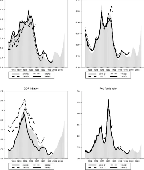
For the models with stochastic volatility to yield density forecasts more accurate than those from models with constant volatilities, it likely needs to be the case that volatility has var-ied significantly over time. Therefore, as a starting point, it is worth considering the estimates of stochastic volatilities from the BVAR-SSPSV model, specifically, time series of reduced-form residual standard deviations (diagonal elements of 0t.5) estimated under the recursive scheme. Figure 1 reports esti-mates (posterior means) obtained with different real-time data vintages. For the key variables of interest, the shaded area provides the volatility time series estimated with data from 1961–2008. The lines provide time series estimated with data samples ending in 1998:Q4, 1991:Q4, and 1984:Q4 (obtained from data vintages of 1999:Q1, 1992:Q1, and 1985:Q1, respec-tively). Overall, the estimates confirm significant time varia-tion in volatility, and generally match the contours of estimates shown by, for example, Cogley and Sargent (2005). In particu-lar, volatility fell sharply in the mid-1980s with the Great Mod-eration. The estimates also reveal a sharp rise in volatility in recent years, reflecting the rise in energy price volatility and the severe recession that started in December 2007.
As might be expected, comparing estimates across real-time data vintages yields some nontrivial differences in volatility es-timates. Data revisions—especially benchmark revisions and large annual revisions—lead to some differences across vin-tages in the stochastic volatility estimates for GDP growth and GDP inflation (a corresponding figure in the online appendix using final-vintage data shows much smaller differences across samples). For growth and inflation, the general contours of volatility are very similar across vintages, but levels can differ somewhat. It remains to be seen whether such changes in real-time estimates are so great as to make it difficult to improve the calibration of density forecasts by incorporating stochastic volatility. Not surprisingly, with the unemployment and funds rates not revised over time, there are few differences across vin-tages in the volatility estimates for these variables.
This section first presents RMSE results for real-time point forecasts. It then presents results for the calibration of real-time density forecasts, including: probabilities of forecasts falling within 70% confidence intervals, the tests of Berkowitz (2001) applied to normal transforms of the PITs, and log predictive scores. (See Mitchell and Wallis2010for a recent summary of density calibration.) Some additional details, including mean forecast errors, charts of PITs and normalized forecast errors for a range of models, and illustrative fan charts, are provided in the online appendix.
5.1 Point Forecasts
Table 1 presents real-time forecast RMSEs for 1985– 2008:Q3, including RMSEs for (constant-variance) AR model forecasts and ratios of RMSEs for a given forecast model or method relative to the AR model. In these blocks, entries with value < 1 mean that a forecast is more accurate than the (constant-variance) AR benchmark. To provide a rough mea-sure of statistical significance, Table2presentsp-values for the null hypothesis that the MSE of a given model is equal to the MSE of the AR benchmark, against the (one-sided) alternative that the MSE of the given model is lower. The online appendix provides p-values for tests of equal accuracy of BVAR fore-casts against each other (as opposed to against the AR bench-mark). These p-values were obtained by comparing the tests of Diebold and Mariano (1995) and West (1996) against stan-dard normal critical values. Monte Carlo results of Clark and McCracken (2009) indicate that the use of a normal distribu-tion for testing equal accuracy in a finite sample (as opposed to in population, which is the focus of other forecast analyses, such as Clark and McCracken2001) can be viewed as a conser-vative guide to inference with models that are nested, as they are here. The standard normal approach tends to be modestly undersized and to have slightly lower power than desired in an asymptotically proper approach, based on a fixed regressor bootstrap that cannot be applied in a BVAR setting.
Consistent with the findings of Clark and McCracken (2008, 2010), the RMSE performance of the conventional BVARs (without variables in gap form and steady-state priors) relative to the benchmark AR models is mixed. For example, at hori-zons of one and two quarters and 1 year, the BVAR forecasts often have RMSEs in excess of the AR RMSE, but for growth, unemployment, and the funds rate, the accuracy of BVAR fore-casts relative to the univariate forefore-casts improves as the forecast
Figure 1. Posterior means of residual standard deviations, real-time vintages. The figure reports estimates of the reduced-form residual variances in the BVAR-SSPSV model (recursive), estimated at various points in time with the vintage of data indicated. The dates given for each line (1985:Q1, 1992:Q1, etc.) correspond to the dates of the data vintages; at each of these points in time, the model was estimated with the indicated vintage, using data through the prior quarter.
Table 1. Real-time forecast RMSEs, 1985–2008:Q3 (RMSEs for benchmark AR models in first panel, RMSE ratios in all others)
h=1Q h=2Q h=1Y h=2Y (a) AR
GDP growth 1.783 1.832 1.320 1.445
Unemployment 0.174 0.313 0.572 1.055
GDP inflation 0.965 1.001 0.669 0.932
Fed funds rate 0.416 0.808 1.489 2.463
(b) AR-SV
GDP growth 1.023 (0.998) 1.023 (0.990) 1.047 (0.988) 1.073 (0.971)
Unemployment 0.996 (0.383) 1.005 (0.588) 1.016 (0.630) 1.026 (0.629)
GDP inflation 1.002 (0.819) 1.001 (0.585) 0.999 (0.343) 0.999 (0.275)
Fed funds rate 0.896 (0.000) 0.943 (0.041) 1.019 (0.700) 1.086 (0.944)
(c) BVAR, recursive
GDP growth 1.242 (0.997) 1.218 (0.986) 1.215 (0.900) 0.924 (0.279)
Unemployment 1.046 (0.728) 1.031 (0.637) 0.991 (0.471) 0.722 (0.002)
GDP inflation 1.102 (0.982) 1.141 (0.993) 1.307 (0.998) 1.573 (0.998)
Fed funds rate 1.157 (0.993) 1.130 (0.920) 1.047 (0.680) 0.964 (0.395)
(d) BVAR, rolling
GDP growth 1.150 (0.989) 1.133 (0.947) 1.086 (0.715) 0.908 (0.318)
Unemployment 1.052 (0.738) 1.015 (0.553) 0.934 (0.295) 0.663 (0.001)
GDP inflation 1.116 (0.981) 1.206 (0.995) 1.461 (0.997) 1.790 (0.994)
Fed funds rate 1.145 (0.997) 1.090 (0.882) 1.021 (0.595) 0.971 (0.405)
(e) BVAR-SSP, recursive
GDP growth 1.160 (0.983) 1.127 (0.942) 1.061 (0.670) 0.899 (0.230)
Unemployment 1.045 (0.729) 1.011 (0.555) 0.947 (0.316) 0.719 (0.013)
GDP inflation 1.051 (0.864) 1.018 (0.634) 1.044 (0.674) 1.078 (0.692)
Fed funds rate 1.144 (0.984) 1.112 (0.881) 0.995 (0.483) 0.859 (0.137)
(f) BVAR-SSP, rolling
GDP growth 1.094 (0.950) 1.049 (0.759) 0.958 (0.382) 0.849 (0.175)
Unemployment 1.008 (0.550) 0.957 (0.283) 0.872 (0.109) 0.674 (0.013)
GDP inflation 1.044 (0.825) 1.017 (0.626) 1.014 (0.561) 1.040 (0.641)
Fed funds rate 1.079 (0.944) 1.012 (0.579) 0.900 (0.071) 0.787 (0.013)
(g) BVAR-SSPSV, recursive
GDP growth 1.076 (0.896) 1.058 (0.797) 0.983 (0.449) 0.884 (0.229)
Unemployment 0.981 (0.374) 0.941 (0.158) 0.901 (0.138) 0.735 (0.012)
GDP inflation 1.034 (0.787) 1.018 (0.650) 0.995 (0.475) 0.994 (0.478)
Fed funds rate 0.959 (0.169) 0.953 (0.217) 0.914 (0.143) 0.829 (0.061)
(h) BVAR-SSPSV, rolling
GDP growth 1.059 (0.887) 1.030 (0.692) 0.940 (0.311) 0.863 (0.191)
Unemployment 0.981 (0.377) 0.927 (0.119) 0.855 (0.042) 0.688 (0.003)
GDP inflation 1.037 (0.791) 1.029 (0.717) 1.003 (0.513) 0.981 (0.412)
Fed funds rate 0.936 (0.044) 0.914 (0.035) 0.863 (0.013) 0.782 (0.009)
NOTE: 1. In each quartertfrom 1985:Q1 through 2008:Q3, vintagetdata (which end int−1) are used to form forecasts for periodst(h=1Q),t+1 (h=2Q),t+3 (h=1Y), and
t+7 (h=2Y). The forecasts of GDP growth and inflation for theh=1Yandh=2Yhorizons correspond to annual percent changes: average growth and average inflation fromtthrough
t+3 andt+4 throught+7, respectively. The forecast errors are calculated using the second-available (real-time) estimates of growth and inflation as the actual data, and currently available measures of unemployment and the federal funds rate as actuals.
2.p-values oft-tests of equal MSE, taking the AR models with constant volatilities as the benchmark, are given in parentheses. These are one-sided Diebold–Mariano–West tests, of the null of equal forecast accuracy against the alternative that the non-benchmark model in question is more accurate. The standard errors entering the test statistics are computed with the Newey–West estimator, with a bandwidth of 0 at the 1-quarter horizon and 1.5×horizon in the other cases.
horizon increases. At the 2-year horizon, BVAR forecasts of these variables are almost always more accurate than AR fore-casts, although the BVAR gains are statistically significant only for unemployment. Consider forecasts of unemployment from the recursive BVAR, in which the RMSE ratio declines from 1.046 at the one-quarter horizon to 0.989 at the 1-year horizon to 0.722 at the 2-year horizon.
Although the pattern is not entirely uniform, for the most part BVARs estimated with rolling samples yield lower RMSEs than BVARs estimated recursively. (The pattern is clearer in the set
of models with steady-state priors.) As examples, the RMSE ratios of 1-year-ahead forecasts of GDP growth are 1.061 with the recursive BVAR-SSP and 0.958 with the rolling BVAR-SSP, and the RMSE ratios of 1-year-ahead forecasts of unemploy-ment are 0.947 with the recursive BVAR-SSP and 0.872 with the rolling BVAR-SSP. Admittedly, although the improvements with a rolling scheme are consistent, they likely are generally too modest to be of statistical significance.
The BVARs with most variables in gap form and steady-state priors generally yield lower RMSEs than conventional
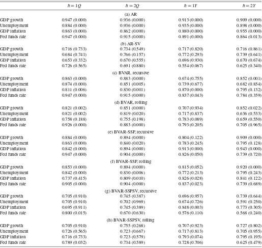
Table 2. Real-time forecast coverage rates, 1985–2008:Q3 (frequencies of actual outcomes falling inside 70% intervals)
h=1Q h=2Q h=1Y h=2Y (a) AR
GDP growth 0.947 (0.000) 0.936 (0.000) 0.913 (0.000) 0.909 (0.000)
Unemployment 0.884 (0.000) 0.936 (0.000) 0.935 (0.000) 0.898 (0.000)
GDP inflation 0.863 (0.000) 0.862 (0.000) 0.880 (0.000) 0.955 (0.000)
Fed funds rate 0.947 (0.000) 0.915 (0.000) 0.891 (0.000) 0.864 (0.013)
(b) AR-SV
GDP growth 0.716 (0.733) 0.734 (0.549) 0.717 (0.820) 0.716 (0.861)
Unemployment 0.684 (0.741) 0.766 (0.157) 0.772 (0.293) 0.739 (0.641)
GDP inflation 0.653 (0.332) 0.670 (0.555) 0.696 (0.930) 0.670 (0.674)
Fed funds rate 0.726 (0.565) 0.691 (0.880) 0.554 (0.067) 0.625 (0.340)
(c) BVAR, recursive
GDP growth 0.863 (0.000) 0.883 (0.000) 0.674 (0.755) 0.852 (0.001)
Unemployment 0.874 (0.000) 0.851 (0.005) 0.739 (0.677) 0.682 (0.854)
GDP inflation 0.811 (0.006) 0.830 (0.001) 0.870 (0.000) 0.795 (0.132)
Fed funds rate 0.947 (0.000) 0.915 (0.000) 0.837 (0.043) 0.784 (0.359)
(d) BVAR, rolling
GDP growth 0.821 (0.002) 0.851 (0.000) 0.707 (0.934) 0.852 (0.022)
Unemployment 0.821 (0.002) 0.819 (0.020) 0.717 (0.837) 0.636 (0.533)
GDP inflation 0.758 (0.188) 0.755 (0.198) 0.783 (0.089) 0.659 (0.550)
Fed funds rate 0.926 (0.000) 0.883 (0.000) 0.793 (0.205) 0.705 (0.965)
(e) BVAR-SSP, recursive
GDP growth 0.884 (0.000) 0.894 (0.000) 0.804 (0.122) 0.909 (0.000)
Unemployment 0.863 (0.000) 0.840 (0.020) 0.783 (0.245) 0.795 (0.128)
GDP inflation 0.842 (0.000) 0.894 (0.000) 0.913 (0.000) 0.943 (0.000)
Fed funds rate 0.947 (0.000) 0.904 (0.000) 0.826 (0.050) 0.739 (0.720)
(f) BVAR-SSP, rolling
GDP growth 0.853 (0.000) 0.894 (0.000) 0.815 (0.052) 0.920 (0.000)
Unemployment 0.842 (0.000) 0.830 (0.006) 0.772 (0.213) 0.795 (0.243)
GDP inflation 0.737 (0.415) 0.809 (0.010) 0.826 (0.028) 0.841 (0.122)
Fed funds rate 0.905 (0.000) 0.904 (0.000) 0.837 (0.023) 0.739 (0.689)
(g) BVAR-SSPSV, recursive
GDP growth 0.705 (0.910) 0.745 (0.387) 0.696 (0.957) 0.739 (0.644)
Unemployment 0.705 (0.910) 0.702 (0.969) 0.674 (0.726) 0.591 (0.250)
GDP inflation 0.695 (0.911) 0.745 (0.389) 0.848 (0.003) 0.773 (0.305)
Fed funds rate 0.800 (0.015) 0.670 (0.630) 0.576 (0.110) 0.568 (0.240)
(h) BVAR-SSPSV, rolling
GDP growth 0.705 (0.910) 0.755 (0.268) 0.707 (0.923) 0.727 (0.802)
Unemployment 0.726 (0.565) 0.723 (0.667) 0.717 (0.813) 0.705 (0.955)
GDP inflation 0.716 (0.733) 0.723 (0.579) 0.793 (0.074) 0.795 (0.195)
Fed funds rate 0.789 (0.032) 0.734 (0.589) 0.728 (0.706) 0.625 (0.479)
NOTE: 1. See the notes to Table1.
2. The table reports the frequencies with which actual outcomes fall within 70 percent bands computed from the posterior distribution of forecasts.
3. The table includes in parenthesesp-values for the null of correct coverage (empirical=nominal rate of 70 percent), based ont-statistics using standard errors computed with the Newey–West estimator, with a bandwidth of 0 at the 1-quarter horizon and 1.5×horizon in the other cases.
BVARs. (For simplicity, much of the discussion that follows refers to these models simply as BVARs with steady-state pri-ors.) This finding is in line with evidence from Clark and McCracken (2008,2010) on the advantage of detrending and evidence from Adolfson et al. (2007), Beechey and Oster-holm (2008), Osterholm (2008), and Wright (2010) on the ad-vantage of steady-state priors. The adad-vantage is most striking for 2-year-ahead forecasts of inflation. Under a rolling estima-tion scheme, BVAR and BVAR-SSP forecasts have RMSE ra-tios of 1.790 and 1.040, respectively. But this advantage (albeit smaller) also applies for most other variables and horizons. At the one-quarter horizon, rolling BVAR and BVAR-SSP
fore-casts of GDP growth have RMSE ratios of 1.150 and 1.094, respectively. At the two-quarter horizon, these RMSE ratios are 1.090 and 1.012. Testp-values, provided in the appendix, indicate that the forecasts from the rolling BVAR-SSP model are significantly more accurate than those from the rolling BVAR model, except in the case of unemployment forecasts at all horizons and GDP growth forecasts at the 2-year hori-zon.
These improvements in RMSE seen at longer horizons are driven in part by smaller mean errors. As detailed in the on-line appendix, mean errors are often lower (in absolute value) for rolling BVARs than recursively estimated BVARs. Mean
rors at longer horizons also tend to be smaller for BVARs with steady-state priors compared with conventional BVARs, espe-cially for inflation and the funds rate.
Adding stochastic volatility to the BVARs with most vari-ables in gap form and steady-state priors tends to further im-prove forecast RMSEs. At the one-quarter horizon, the recur-sive BVAR-SSP yields RMSE ratios of 1.160 for GDP growth and 1.144 for the funds rate, whereas the recursive BVAR-SSPSV yields corresponding ratios of 1.076 and 0.959. At the 1-year horizon, the recursive BVAR-SSP yields RMSE ratios of 1.061 for GDP growth and 0.995 for the funds rate, whereas the recursive BVAR-SSPSV yields corresponding ratios of 0.983 and 0.914. Based on the RMSE metric, the rolling BVAR-SSPSV is probably the single best multivariate model, produc-ing, for example, the most instances of rejections of equal accu-racy with the AR benchmark. D’Agostino, Gambetti, and Gian-none (2009) similarly found that including stochastic volatility in a BVAR (in their case, a model with time-varying parame-ters) improved the accuracy of point forecasts.
5.2 Density Forecasts: Interval Forecasts
In light of central bank interest in uncertainty surrounding forecasts, confidence intervals, and fan charts, a natural starting point for forecast density evaluation is interval forecasts—that is, coverage rates. Recent studies, such as that of Giordani and Villani (2010), used interval forecasts as a measure of the cali-bration of macroeconomic density forecasts. Table2reports the frequency with which real-time outcomes for growth, unem-ployment, inflation, and the federal funds rate fall inside 70% highest posterior density intervals estimated in real time with the BVARs (the online appendix provides charts of time series of the intervals). Accurate intervals should result in frequen-cies of about 70%. A frequency of greater than (less than) 70% means that on average over a given sample, the posterior density is too wide (narrow). The table includesp-values for the null of correct coverage (empirical=nominal rate of 70%), based ont-statistics. Thesep-values are provided as a rough gauge of the importance of deviations from correct coverage. The gauge is rough because the theory underlying Christofferson’s (1998) test abstracts from forecast model estimation—that is, parame-ter estimation error—whereas all forecasts considered in this paper are obtained from estimated models.
As Table2 shows, the (constant-variance) AR, BVAR, and BVAR-SSP intervals tend to be too wide, with actual outcomes falling inside the intervals much more frequently than the nom-inal 70% rate. For example, for the one-quarter-ahead forecast horizon, the recursive BVAR-SSP coverage rates range from 84.2% to 94.7%. Based on the reported p-values, all of these departures from the nominal coverage rate appear to be statis-tically meaningful. Using the rolling estimation scheme yields slightly to somewhat more accurate interval forecasts (but the departures remain sufficiently large to deliver low p-values, with the exception of the inflation forecasts), with BVAR-SSP coverage rates ranging from 73.7% to 90.5% at the one-step-ahead horizon. In some cases, the interval forecasts become more accurate at the 1-year or 2-year horizons, with coverage rates closer to 70%; for example, in the case of unemployment
forecasts from the rolling BVAR-SSP, the coverage rate im-proves from 84.2% at the one-quarter horizon to 77.2% at the 1-year horizon.
Adding stochastic volatility to the AR models and to the BVAR with a steady-state prior materially improves the cal-ibration of the interval forecasts. For the one-quarter-ahead forecast horizon, the AR-SV coverage rates range from 65.3% to 72.6%, down from the AR coverage rate range of 86.3%– 94.7%. At the same horizon, the rolling BVAR-SSPSV cover-age rates range from 70.5% to 78.9%, compared with the rolling BVAR-SSP’s range of 73.7%–90.5%. With the BVAR-SSPSV stochastic volatility specifications, for growth, unemployment, and inflation forecasts, thep-values for one-step-ahead cover-age all exceed 0.56. But covercover-age remains too high in the case of the funds rate, at roughly 80%—materially better than in the models without stochastic volatility, but still too high. At the 1-year-ahead horizon, the rolling BVAR-SSPSV coverage rates range from 70.7% to 79.3%, compared to the rolling BVAR-SSP’s range of 77.2%–83.7%.
For a given model, differences in coverage across horizons likely reflect a variety of forces, making a single explanation difficult. One force is sampling error. Even if a model were correctly specified, random variation in a given data sample could cause the empirical coverage rate to differ from the nom-inal. Sampling error increases with the forecast horizon, due to the overlap of forecast errors for multistep horizons (effec-tively reducing the number of independent observations relative to the one-step horizon). Of course, an increased sampling er-ror across horizons will translate into reduced power to detect departures from accurate coverage.
Another force is the role of (implied or directly estimated) steady states in forecasts at different horizons. As emphasized by, for example, Kozicki and Tinsley (2001a, 2001b), as the horizon increases, forecasts are increasingly determined by the steady states. Some of the apparent improved coverage shown in Table2occurring as the horizon grows (especially for infla-tion and the funds rate) is due to an increased role of implied or estimated steady states that are too high. Consider, for exam-ple, forecasts of the federal funds rate from the rolling BVAR model. The one-quarter horizon coverage rate of 92.6% indi-cates the interval forecast is far too wide. However, the model’s implied steady-state funds rate level is too high. As the horizon increases, the forecasts from the model systematically overstate the funds rate. The bias of the point forecast from the model rises (in absolute value) from−0.160 at the one-quarter hori-zon to−1.249 percentage points at the 2-year horizon (online appendix). At the 2-year horizon, the forecast interval is likely still too wide, but the whole interval is pushed up by the bias of the point forecasts. As a result, some observations fall be-low the be-lower band of the interval, raising the reported coverage rate, but entirely in one tail and not in the other. Whereas 29.5% of the actual observations fall outside the 70% interval at the 2-year horizon, 27.3% fall below the lower tail, and only 2.2% are above the upper tail. In such cases, of course, the nominal improvement in reported coverage does not actually represent better density calibration. Note that this particular force should not create similar patterns in the log scores, a broader measure of density calibration, reported below.
5.3 Density Forecasts: Normal Transforms of PITs
Normal transforms of PITs also can provide useful indi-cators of the calibration of density forecasts. The normalized forecast error is defined as−1(zt+1), wherezt+1denotes the
PIT of a one-step-ahead forecast error and−1is the inverse of the standard normal distribution function. As developed by Berkowitz (2001), the normalized forecast error should be an independent standard normal random variable, because the PIT series should be an independent uniform(0, 1) random variable. Berkowitz developed tests based on the normality of the nor-malized errors. These tests, which have better power than tests based on the uniformity of the PITs, have been used in recent studies such as Clements (2004) and Jore, Mitchell, and Va-hey (2010). Giordani and Villani (2010) also suggested that time series plots of the normalized forecast errors provide use-ful qualitative evidence of forecast density calibration, and may reveal advantages or disadvantages of a forecast not evident from alternatives such as PIT histograms.
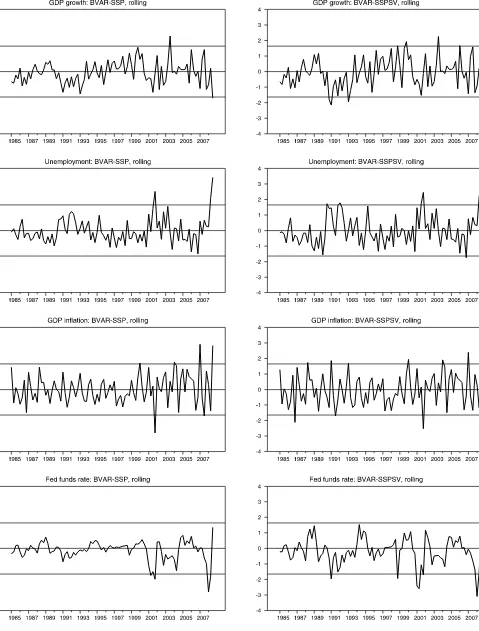
Figure 2 reports time series of normalized forecast errors from the rolling BVAR-SSP and rolling BVAR-SSPSV spec-ifications, with bands representing 90% intervals for the nor-mal distribution. (Nornor-malized errors for other models, consis-tent with the subset of presented results, are provided in the online appendix.) Normalized errors from BVARs without sto-chastic volatility demonstrate seemingly important departures from the standard normal distribution. Many of the charts show that the normalized errors have variances well below 1, nonzero means, and serial correlation. The most dramatic examples are for forecasts of the funds rate (from the rolling BVAR-SSP); less dramatic, although still clear, examples include forecasts of GDP growth and unemployment from the rolling BVAR-SSP. The transforms look best (i.e., closest to the standard normal conditions) for forecasts of GDP inflation, which are clearly more variable.
The normalized forecast errors from BVARs with stochas-tic volatility look much better, with larger variances and means closer to 0. In the case of GDP growth, variability of normal-ized errors is clearly greater for the BVAR-SSPSV specifica-tions than the BVAR-SSP model, and the mean also appears to be closer to 0. Qualitatively, Giordani and Villani (2010) ob-tained similar results when comparing forecasts of GDP growth from a constant parameter AR model to forecasts from a model that allows coefficient and variance breaks. However, even with stochastic volatility, there remains an extended period of nega-tive errors in the early 1990s, which implies serial correlation in the normalized errors. The same basic pattern applies to the nor-malized errors of unemployment forecasts. The results shown in Figure2 for inflation forecasts also suggest that stochastic volatility improves the behavior of normalized errors, although not as dramatically as for GDP growth and unemployment. Fi-nally, in the case of federal funds rate forecasts, allowing sto-chastic volatility also significantly increases the variance of the normalized errors, but seems to leave strong serial correlation.
For a more formal assessment, Table3 reports various test metrics, including the variances of the normalized errors, along withp-values for the null that the variance equals 1; the means of the normalized errors, along withp-values for the null of a zero mean; the AR(1) coefficient estimate and itsp-value, ob-tained by a least squares regression including a constant; and
the p-value of Berkowitz’s (2001) likelihood ratio test for the joint null of zero mean, unity variance, and no [AR(1)] serial correlation.
The tests confirm that without stochastic volatility, variances are materially less than 1, means are sometimes nonzero, and serial correlation can be considerable. For example, with the recursive BVAR-SSP model, the variances of the normalized forecast errors range from 0.205 (funds rate) to 0.636 (infla-tion), withp-values close to 0. With the same model, the AR(1) coefficients are 0.310 for GDP growth, 0.393 for unemploy-ment, −0.198 for inflation, and 0.674 for the funds rate; the corresponding p-values are all close to 0, except in the case of inflation, for which thep-value is 0.051. However, particu-larly in terms of means and variances, the rolling scheme fares somewhat better than the recursive. Not surprisingly, given re-sults such as these for means, variances, and AR(1) coefficients, thep-values of the Berkowitz (2001) test are nearly 0 for con-stant variance AR, recursive and rolling BVAR, and recursive and rolling BVAR-SSP forecasts, with the exception of rolling forecasts of GDP inflation.
By the formal metrics, as by the charts, allowing stochas-tic volatility improves the calibration of density forecasts. In the case of the recursive BVAR-SSPSV specification, the vari-ances of the normalized forecast errors range from 0.848 (fed-eral funds rate) to 1.030 (inflation), withp-values of 0.223 or greater. The AR(1) coefficients are all lower (in absolute value) for forecasts from the recursive BVAR-SSPSV than from the recursive BVAR-SSP specification. For unemployment and in-flation, thep-values of the Berkowitz test exceed 0.10. For GDP growth, thep-value of the test exceeds 0.05. Adding stochastic volatility to AR models yields a qualitatively similar improve-ment (relative to constant-variance AR models) in the proper-ties of normalized forecast errors, with the forecasts passing the Berkowitz test for all but the funds rate, for which the violation appears to be due to serial correlation in the normalized error.
5.4 Density Forecasts: Log Predictive Density Scores
The overall calibration of the density forecasts can be mea-sured most broadly with log predictive density scores, as used by Geweke and Amisano (2010). For computational tractabil-ity, I compute the log predictive density score based on the Gaussian (quadratic) formula given by Adolfson, Linde, and Villani (2005), under which a lower score implies a better model. For brevity, I report only average log scores for the full vector of variables of interest: GDP growth, unemployment, in-flation, and the federal funds rate. The online appendix provides scores for each individual variable.
To help provide a rough gauge of the significance of score differences, I rely on the methodology developed by Amisano and Giacomini (2007), and report p-values for selected dif-ferences in mean scores, under the null of a zero mean. Be-cause the theoretical basis for the test provided by Amisano and Giacomini requires forecasts estimated with rolling sam-ples of data (but takes into account the effects of uncertainty associated with the estimation of model parameters), I apply the test only to pairs of forecasts from models estimated with the rolling scheme: BVAR against BVAR-SSP, BVAR against BVAR-SSPSV, and BVAR-SSP against BVAR-SSPSV.
Figure 2. normalized forecast errors from selected models. The normalized, 1-step ahead forecast errors shown are defined as−1(zt+1), wherezt+1denotes the probability integral transform of a one-step ahead forecast error (generated in real time) and−1is the inverse of the standard normal distribution function. The horizontal lines included in the charts represent 90% intervals for the normal distribution.
Table 3. Tests of normalized errors of 1-step ahead real-time forecasts, 1985–2008:Q3
Variance (p-value) Mean (p-value) AR(1) coef. (p-value) LR testp-value (a) AR
GDP growth 0.269 (0.000) −0.089 (0.133) 0.060 (0.537) 0.000
Unemployment 0.433 (0.000) 0.016 (0.823) −0.150 (0.235) 0.000
GDP inflation 0.482 (0.000) 0.007 (0.911) 0.071 (0.516) 0.000
Fed funds rate 0.278 (0.000) −0.025 (0.738) 0.523 (0.002) 0.000
(b) AR-SV
GDP growth 0.832 (0.139) −0.164 (0.111) 0.052 (0.611) 0.179
Unemployment 0.960 (0.772) 0.125 (0.254) −0.133 (0.226) 0.356
GDP inflation 1.069 (0.596) −0.001 (0.990) 0.119 (0.252) 0.677
Fed funds rate 0.974 (0.888) −0.094 (0.476) 0.333 (0.003) 0.009
(c) BVAR, recursive
GDP growth 0.506 (0.000) −0.334 (0.001) 0.337 (0.000) 0.000
Unemployment 0.527 (0.000) 0.162 (0.151) 0.401 (0.000) 0.000
GDP inflation 0.672 (0.001) −0.169 (0.004) −0.204 (0.054) 0.002
Fed funds rate 0.200 (0.000) −0.165 (0.022) 0.667 (0.000) 0.000
(d) BVAR, rolling
GDP growth 0.534 (0.000) −0.107 (0.320) 0.266 (0.008) 0.000
Unemployment 0.675 (0.070) 0.140 (0.254) 0.381 (0.007) 0.000
GDP inflation 0.901 (0.512) −0.103 (0.228) −0.143 (0.172) 0.332
Fed funds rate 0.400 (0.000) −0.192 (0.026) 0.537 (0.002) 0.000
(e) BVAR-SSP, recursive
GDP growth 0.443 (0.000) −0.226 (0.021) 0.310 (0.001) 0.000
Unemployment 0.555 (0.001) 0.096 (0.406) 0.393 (0.001) 0.000
GDP inflation 0.636 (0.000) −0.065 (0.269) −0.198 (0.051) 0.006
Fed funds rate 0.205 (0.000) −0.159 (0.034) 0.674 (0.000) 0.000
(f) BVAR-SSP, rolling
GDP growth 0.517 (0.000) −0.051 (0.600) 0.204 (0.047) 0.000
Unemployment 0.648 (0.037) −0.008 (0.942) 0.332 (0.034) 0.001
GDP inflation 0.880 (0.453) 0.027 (0.726) −0.163 (0.097) 0.369
Fed funds rate 0.407 (0.000) −0.136 (0.136) 0.546 (0.001) 0.000
(g) BVAR-SSPSV, recursive
GDP growth 0.852 (0.223) −0.158 (0.215) 0.189 (0.065) 0.063
Unemployment 0.921 (0.614) 0.024 (0.856) 0.203 (0.079) 0.269
GDP inflation 1.030 (0.805) −0.089 (0.265) −0.124 (0.206) 0.540
Fed funds rate 0.848 (0.361) −0.225 (0.097) 0.494 (0.000) 0.000
(h) BVAR-SSPSV, rolling
GDP growth 0.851 (0.186) −0.081 (0.509) 0.182 (0.063) 0.172
Unemployment 0.878 (0.446) 0.015 (0.910) 0.266 (0.026) 0.075
GDP inflation 1.003 (0.980) −0.014 (0.868) −0.123 (0.184) 0.710
Fed funds rate 0.759 (0.201) −0.188 (0.116) 0.483 (0.000) 0.000
NOTE: 1. See the notes to Table1.
2. The normalized forecast error is defined as−1(zt+1), wherezt+1denotes the PIT of the one-step ahead forecast error and−1is the inverse of the standard normal distribution
function.
3. The first column reports the estimated variance of the normalized error, along with ap-value for a test of the null hypothesis of a variance equal to 1 (computed by a linear regression of the squared error on a constant, using a Newey–West variance with 3 lags). The second column reports the mean of the normalized error, along with ap-value for a test of the null of a mean of zero (using a Newey–West variance with 5 lags). The third column reports the AR(1) coefficient and itsp-value, obtained by estimating an AR(1) model with an intercept (with heteroskedasticity-robust standard errors). The final column reports thep-value of Berkowitz’s (2001) likelihood ratio test for the joint null of a zero mean, unity variance, and no [AR(1)] serial correlation.
The average log predictive density scores, reported in Ta-ble 4, show that a rolling estimation scheme almost always yields better (lower) log scores than a recursive estimation scheme, although sometimes only slightly so. For example, with the BVAR-SSP model, the rolling scheme yields log scores of 8.526 at the one-quarter horizon and 10.372 at the 1-year horizon, compared with the recursive scheme’s correspond-ing log scores of 8.772 and 10.732. In addition, uscorrespond-ing gap forms for most variables and a steady-state prior usually im-proves log scores; regardless of the estimation scheme
(recur-sive or rolling), log scores are typically lower for the BVAR-SSP model than for the BVAR model. Continuing with the same example, the rolling BVAR has log scores of 8.600 at the one-quarter horizon and 10.767 at the 1-year horizon (compared with the rolling BVAR-SSP’s scores of 8.526 and 10.327.
Allowing stochastic volatility offers improvements in log scores that seem especially considerable at short horizons. The log scores of the rolling BVAR-SSPSV are 7.345 for one quar-ter, 9.716 for two quarters, 10.019 for 1 year, and 12.380 for 2 years, compared with the rolling BVAR-SSP model’s log
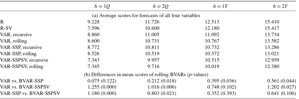
Table 4. Real-time forecast average log scores, 1985–2008:Q3
h=1Q h=2Q h=1Y h=2Y (a) Average scores for forecasts of all four variables
AR 9.228 11.726 12.513 15.410
AR-SV 7.596 10.600 12.180 15.417
BVAR, recursive 8.860 11.005 11.092 13.734
BVAR, rolling 8.600 10.731 10.767 13.582
BVAR-SSP, recursive 8.772 10.811 10.732 13.286
BVAR-SSP, rolling 8.526 10.519 10.372 13.021
BVAR-SSPSV, recursive 7.343 9.957 10.515 12.959
BVAR-SSPSV, rolling 7.345 9.716 10.019 12.380
(b) Differences in mean scores of rolling BVARs (p-values)
BVAR vs. BVAR-SSP 0.075(0.122) 0.212(0.018) 0.395(0.036) 0.561(0.044)
BVAR vs. BVAR-SSPSV 1.255(0.000) 1.016(0.006) 0.748(0.102) 1.202(0.027)
BVAR-SSP vs. BVAR-SSPSV 1.180(0.000) 0.803(0.021) 0.352(0.393) 0.641(0.106)
NOTE: 1. See the notes to Table 1.
2. The entries in the upper panel of the table are average values of log predictive density scores, computed with the Gaussian (quadratic) formula given in Adolfson, Linde, and Villani (2005), under which a lower score implies a better model.
3. The entries in the lower panel of the table are differences in average log predictive density scores andp-values from Amisano and Giacomini (2007) tests of equal average scores. The tests andp-values are computed by regressions of differences in log scores (time series) on a constant, using the Newey–West estimator of the variance of the regression constant (with a bandwidth of 0 at the 1-quarter horizon and 1.5×horizon in the other cases). All of the test results are based on forecasts from models estimated with rolling samples of data, per the assumptions of Amisano and Giacomini (2007).
scores of 8.526, 10.519, 10.372, and 13.021, respectively. In-cluding stochastic volatility in AR models also significantly im-proves log scores relative to constant-variance AR models; for instance, at the one-quarter horizon, the log score for the AR-SV model was 9.228, compared with 7.596 for the AR model. For the vector of four variables being forecast, the BVARs with stochastic volatility score better than the AR models with sto-chastic volatility, especially at longer horizons. This difference is likely due to covariances among forecasts that the BVARs capture better. The online appendix shows that for each individ-ual variable separately, the AR-SV and BVAR-SSPSV scores are broadly comparable.
Thep-values of the differences in average log scores reported in Table4 indicate that the improvements in density forecasts from BVARs associated with stochastic volatility are statisti-cally meaningful at short horizons, but mixed at longer hori-zons. Comparing the (rolling in all cases) BVAR-SSP against the BVAR-SSPSV shows the following differences in average log scores: 1.180, with ap-value of 0.000 for one quarter; 0.803, with ap-value of 0.021, for two quarters; 0.352, with ap-value of 0.393, for 1 year; and 0.641, with a p-value of 0.106, for 2 years. Based on this evidence, it seems reasonable to con-clude that modeling stochastic volatility significantly improves the calibration of density forecasts, although more convincingly at shorter horizons than at longer horizons.
6. CONCLUSION
Central banks and other forecasters have become increas-ingly interested in various aspects of density forecasts. How-ever, sharp changes in macroeconomic volatility, including the Great Moderation and the more recent rise in volatility asso-ciated with greater variation in energy prices and the deep re-cession, pose significant challenges to density forecasting. Ac-cordingly, this paper has examined, using real-time data, den-sity forecasts of GDP growth, unemployment, inflation, and the
federal funds rate from BVAR models with stochastic volatil-ity. Drawing on previous research to improve the accuracy of point forecasts, the model of interest includes most vari-ables in a gap, or deviation from trend, form and incorpo-rates informative priors on the steady states of the model vari-ables.
The evidence presented in the paper demonstrates that adding stochastic volatility to the BVAR with most variables in gap form and a steady-state prior materially improves the real-time accuracy of density forecasts and more modestly improves the accuracy of point forecasts. The paper also shows that adding stochastic volatility to univariate AR models materially im-proves density forecast calibration relative to AR models with constant variances. The density evidence includes interval fore-casts (coverage rates), time series plots of normal transforms of PITs, various tests applied to normal transforms of PITs, and log predictive density scores. In the absence of stochas-tic volatility, models estimated with rolling samples of data are more accurate in density forecasting than models estimated re-cursively; however, modeling stochastic volatility yields larger gains in forecast accuracy.
SUPPLEMENTARY MATERIALS
Appendix: File providing additional detail on data used in the paper and some additional results. (Clarksupplement.pdf)
ACKNOWLEDGMENTS
The author gratefully acknowledges helpful conversations with Taeyoung Doh, John Geweke, Mattias Villani, and Chuck Whiteman and comments from anonymous referees, Gianni Amisano, Marek Jarocinski, Michael McCracken, Par Oster-holm, Shaun Vahey, seminar participants at the Federal Reserve Banks of Boston, Chicago, and Kansas City, and participants at the 2010 ECB-Bundesbank-EABCN workshop on forecast-ing techniques. Special thanks are due to Mattias Villani for