Automatic Identification of General Vector Error Correction Models

Automatic Identification of General Vector Error

Correction Models

Ignacio Arbués, Ramiro Ledo, and Mariano Matilla-García

Abstract

There are a number of econometrics tools to deal with the different types of situations in which cointegration can appear: I(1), I(2), seasonal, polyno- mial, etc. There are also different kinds of Vector Error Correction models related to these situations. The authors propose a unified theoretical and practical framework to deal with many of these situations. To this aim: (i) they introduce a general class of models and (ii) provide an automatic method to identify models, based on estimating the Smith form of an autoregressive model. Their simulations suggest the power of the new proposed methodology. An empirical example illustrates the methodology.

(Published in Special Issue Recent Developments in Applied Economics)

JEL C01 C22 C32 C51 C52

Keywords Time series; unit root; cointegration; error correction; model identification; Smith form

Authors

Ignacio Arbués, Ministerio de Industria, Energía y Turismo and Instituto Complutense de

Análisis Económico, Madrid, Spain

Ramiro Ledo, UNED and Universidad Complutense de Madrid, Facultad de Ciencias

Económicas y Empresariales, Departamento de Economía Aplicada II, Spain

Mariano Matilla-García, UNED, Departamento de Economía Aplicada Cuantitativa,

Paseo Senda del Rey, 11, 28040, Madrid, Spain,

1 Introduction

The basis of the theory of cointegration was laid out in a surge of articles about the late eighties and early nineties, preceded by the seminal paper by Granger (1981). By the mid-nineties, there was a relatively complete theoretical framework for I(1) (Engle and Granger, 1987; Johansen, 1988; Johansen and Juselius, 1990), I(2) cointegration (Johansen, 1992; Paruolo, 1996), multicointegration (Granger and Lee, 1989) and seasonal cointegration (Hylleberg et al., 1990).

Since then, much of the attention in cointegration theory has been focused on panel data (Levin and Lin, 1993; Levin et al., 2002) or on fractional cointegration (Engle and Granger, 1987; Granger and Joyeux, 1980). Latest developments are focused on particular cases as cointegration in dynamic panels (Yu and Lee, 2010), or panel data multicointegration (Worthington and Higgs, 2010).

Also, some contributions have been made to the foundations and algebraic theory of multivariate integrated processes (Franchi, 2006, 2007). A concern that may explain the persistence of interest in the algebra of cointegration is the perceived necessity of a unifying theoretic framework for all situations.

fractional integration poses more difficulties from the theoretical point of view, whereas the algorithms we use are not well-suited to panel data.

The second contribution (Section 3) is an automatic method to identify GVEC models based on an estimate of the SF of the autoregressive model. We show by means of Monte Carlo simulations (Section 4) that our method works better than the Johansen test in the restricted cases in which the latter applies. But of course, our method has also the advantage that it can detect other situations. This is the case in the practical example of Section 5, where our algorithm detects both seasonal cointegration and higher order of integration. Therefore, in series that have a marked seasonal behavior, with our method it is no longer necessary to do a cointegration analysis with the seasonally adjusted series, as is sometimes done.

2 General Vector Error Correction Models

In this section, we generalize some fundamental results of the representation of cointegrated variables by means of VEC models. We will denote polynomials and power series using the inderminatez. When we use them to define autoregressive or ARMA models, we substitute the backshift operatorBforz, so for example φ(z) =φ0+. . .+φpzp, butφ(B)yt =φ0yt+. . .+φpyt−p. Sometimes, when the

context makes clear thatφ is a polynomial, we can drop the indeterminate for ease of notation. The same applies for vectors and matrices whose entries are polynomials or power series.

Assumption 1. Let yt be a n×1random vector, s be a positive integer and d(z)a real polynomial such that all its roots belong to{ωk}sk−=10whereωk=exp 2πik/s and d(B)yt is stationary and purely nondeterministic.

The fact that we limit the roots of d to that set is just for convenience, as the most common cause of unit roots other than the unity is seasonal integration. Hence,scan be interpreted as the number of observations per year (or per week in the case of daily data). All the subsequent developments can easily be adapted to the general case, although most applications do not require that.

Under assumption 1, if the multiplicity of ωk is dk we can say that yt is

We say that yt is polynomially cointegrated of order jat ωk when there exists

a polynomial vector a(z) such that a(B)′yt is Ik(dk−j). There can be several

cointegration relationships foryt. For eachkand j, let us say there is a setA of

such vectors with exactlyrk,j elements and{a(ωk)}a∈A is linearly independent. For the sake of generality, we do not require that all the components ofyt have the

same order of integration, so there may be trivial cointegration relationships. Then, ifyt = (y1,t,y2,t)′, wherey1,t∼I(1)andy2,t∼I(0), a trivial cointegrating vector

would be(0,1)′. For convenience, we can say thatyt is cointegrated of order 0 with

rankn, sork,0=n. Clearlyrk,j≥rk,j+1and there is some jfrom whichrk,j=0

onwards. We callrk,jcointegration ranks.

Assumption 2. The Wold representation of d(B)yt isΨ(B)εt, whereΨ(z)is ratio-nal, that is, its entries are polynomial fractions.

Now, we will present our generalization of the Granger Representation Theo-rem (GRT) as in Engle and Granger (1987). First, we adapt statements (1)–(3).

Proposition 1. If assumptions 1 and 2 hold and yt has cointegration ranks rk,j, then

(a) Ψ(z) =U(z)D(z)V(z), wheredetU(z)anddetV(z)have no roots in the closed unit circle, D(z) =D0(z)·. . .·Ds−1(z)and

Dk(z) =



  

Isk,0 0 0 . . .

0 1−ω−1

k z

Isk,1 0 . . .

0 0 1−ω−1

k z

2

Isk,2 . . .

. . . .



  

where sk,j=rk,j−rk,j+1. D(z)is called the Smith form1ofΨ(x). Conversely, if the SF is as above, then yt has cointegration ranks rk,j.

(b) There is a VARMA representation A(B)yt =m(B)εt such that m(z)is a polynomial. If D divides d, then the SF of A(z)is d(z)D(z)−1_{and m(z)has no unit roots. In this} case, there is also the infinite VAR representationΦ(B)yt=m(B)−1A(B)yt=εt.

(c) There are full rank n×rk,j polynomial matricesα(z)andγ(z)such thatα(z)′Ψ(z) andΨ(z)γ(z)have jth-order zeros atωk.

Proof. See Appendix A.

Statements (a) and (b) are of paramount importance for our results, because they mean that the cointegration structure ofyt can be entirely obtained from the

SF ofΨ(z)orΦ(B). In order to distinguish both diagonal matrices we can use

Proposition 2. In the conditions of Proposition 1, yt satisfies the model

Γ(B)∆_h(B)yt =

We will see now some examples of well-known models that are particular cases of GVEC. Whenyt isI(1), the simplest case occurs whenDΦ(z) =diag(1− z, . . . ,1−z). Then, the components ofyt are not actually cointegrated. A stable

VAR model can be fitted for their differences(∇y_t1, . . . ,∇yn_t). In a similar fashion, ifyt is seasonally integrated andDΦ(z) =diag(1−zs, . . . ,1−zs), a stable VAR is

We encounter classicalI(1)cointegration when

If we allow unit roots other than unity, in particular seasonal roots, the picture is much more complicated. However, there is a particular case that has been already described in the literature. Let us assume thatyt represents quarterly data, sos=4.

If

then (1) boils down to the model in section 4 of Hylleberg et al. (1990). With our notation,

If we calculate the SF ofΨ(B)inR[z], we get the representation

Note that the alternative representation by Haldrup and Salmon (1998),

∇

is in a greater ring, that contains∇−1_{. The conditionD}Ψ_{|dis violated because the} second element∇2_{in the diagonal of the SF ofΨ(B)does not divide the operator∇} that we use to make(pt,st)stationary. Nevertheless, in order to get a representation

without a moving average part this problem can be circumvented by modeling the integrated vector∇_(Pt,St)′_{= (p}

This is the I(2) cointegration case withr2=0. In fact, we can follow the construc-tive proof of Proposition 2 and arrive to the model

∇2

Here we can see the two cointegration relations. The second row means that sales and inventory are cointegrated, and the sum of the two rows gives the relation between sales and production.

We will get asymptotic properties of of the least squares estimation of models of the form of (1) in the case thatΓ(B) is of finite order, but first we need an additional assumption.

Proposition 3. Let yt satisfy model (1), whereΓ(z)is a polynomial matrix andεt fulfils assumption 3. In addition, for simplicity we assume that d|D, so m(z) =1

. Let us stack the coefficients of model (1) as β = [Γ:Π] with Γ= [Γ₁, . . .],

Π= [Π(1)_{, . . . ,Π}(h)_]andΠ(j)_{= [Π}(j)

11, . . .]and letβˆ = [Γˆ : ˆΠ]be the least squares estimator ofβ. Then,βˆ →p β and

T1/2(Γˆ−Γ) →d N(0,Ξ) (3)

LT(Πˆ −Π) = Op(1) (4)

where LT=diag(TqjkℓIn)jkℓ, qjkℓis the minimum multiplicity of the unit roots of

∆_jkℓ(z).

Proof. See Appendix A.

It is likely that consistency could be proved in the case that the trueΓ(B)has infinite order. That would require the order of the estimate ˆΓ(B) to diverge to infinity at a certain rate, as in Lewis and Reinsel (1985).

This result should be extended to allow the presence of moving average terms in the model. The results of Barrio Castro and Osborn (2011), suggest that significant improvements could be achieved with this generalization, that could be attempted following the lines of Yap and Reinsel (1995).

3 Identification

We have built an R package to automatically identify and estimate GVEC models. This package can be obtained from the corresponding author until it is uploaded to a public repository. The main steps of the procedure are: (i) estimate a VAR repre-sentationΦ(B)yt =εt; (ii) estimating the SF ofΦ(z)and (iii) applying Proposition

2 to obtain the GVEC model.

This procedure resembles the unit root determination method of the program TRAMO2, albeit with the additional complication that polynomial matrices cannot

2 _{Current versions of this program, together with SEATS have been developed by Agustín Maravall}

be factorized as simply as polynomials. The method of TRAMO is described in the introductory notes by Maravall (2008).

Steps (i) and (iii) are straightforward. What we need now is a way to estimate the SF of a polynomial or rational matrix. In fact, we will describe a method to estimate the SF in any ring in which we can perform the Euclidean division (Euclidean ring). In Section 3.1 we will describe the algorithm to do that. In Section 3.2 we adapt the algorithm to identify GVEC models.

3.1 Smith form

The existence of the SF of a matrix with elements in a Principal Ideal Domain is guaranteed by Proposition 2.11 in Hungerford (1980).

Let A be a matrix with entries in a ring Rand D=diag(d1, . . . ,dr,0, ...,0)

its SF. Although the SF is not strictly unique, the ideal(di)generated by theith

element of the main diagonal ofDis unique, sodiis unique up to multiplication

by an invertible element ofR. Hence, to achieve uniqueness ofD, it is necessary to impose additional constraints. For example, in the ringR[z]of polynomials overR we may set the coefficient of the highest order term equal to unity, that is, to force

dito be monic.

In general, we will denote byR1a subset ofRsuch that for anya∈Rthere is a uniquea1∈R1witha=ua1anduinvertible (R1always exists because by the axiom of choice, we can pick one element from each equivalence class with respect to the relationa∼b⇔ ∃u∈R,a=u−1b). Thus, whenR=R[z],R1is the set of the monic polynomials. We define a functiona7→u(a)such thatu(a)is invertible andu(a)a∈R1.

The proof of the existence of the SF consists of showing that there is an algorithm that by means of elementary operations transformsAintoD. We will call that the ’exact algorithm’ for reasons that will be obvious later. In the next subsection, we will present a stylized description of the algorithm.

We say thatRis a Euclidean Ring with degree functionϕ:R− {0} 7→Nwhen: (i) pq6=0 impliesϕ(pq)≥ϕ(p)and (ii) for any p,q∈R, there are somem,r∈R

such thatp=mq+randr=0 orϕ(r)<ϕ(r).

LetMn(R)be the ring of then×nmatrices with elements inRandA∈Mn(R).

(a) Exchange rowsiand j.

(b) Exchange columnsiand j.

(c) Addctimes rowito row j, wherecis the quotient of the Euclidean division ofai jbyaiiandaii∈R1.

(d) Addctimes columnito column j, wherecis the quotient of the Euclidean division ofajibyaiiandaii∈R1.

(e) Multiply columnior row jbyu(aii).

Proposition 4. There exist algorithms to obtain the SF of a matrix over an Eu-clidean ring that have the following form:

(i) e0=1,A(0)=A.

(ii) For k>0,

ek= f0(ek−1,A(k−1)) (5) A(k)=g(ek−1,A(k−1)) (6)

(iii) The algorithm stops when ek=0and D=A(k),

where f0:N×Mn(R)7→Nand g:N×Mn(R)7→Mn(R)satisfy

(a) If∀i,j, either Ai,j=Bi j=0or Ai,j,Bi j6=0, then f0(e,A) = f0(e,B).

(b) g(e,A)is obtained from A by performing an admissible operation that depends on e.

Proof. See Appendix A.

Condition (a) means that f0 depends only on (1) its first argument and (2) which elements of the second argument are zero.

Assume that the ringRis endowed with a topology (that makes the sum and product continuous) so that we can speak of random elements inR. Then, for a certain matrixA, we may have an estimate obtained with a sample of sizeT, say

ˆ

AT. Furthermore, suppose ˆAT is consistent in probability. We are interested in the

SFDofA, so we could in principle, proceed by applying the exact algorithm to ˆ

AT obtaining a ˆDT with the hope that when ˆAT p →A, ˆDT

p

→D. Unfortunately, it is easy to prove with an example that this does not work. Let us consider the case of a 2×2 matrix with elements in the ring of the polynomials overR. In order to achieve uniqueness, we set the highest order coefficient equal to one. Assume that

ˆ

LetMn(R)be the ring (andR-module) of then×nmatrices with entries inR.

In analogy with the usual notation in linear algebra, we will write forA∈Mn(R),

kAk= sup a∈Rn_,a6=0

kAak

kak . (7)

where fora= (a1, . . . ,an),kak= ∑j|aj|2

1/2

. The finiteness of the supremum in (7) can be proved in a similar fashion as in the vector space case. From now onwards, convergence of elements of R and matrices will be referred to the topologies generated by| · |andk · krespectively.

Now, we can introduce the ’approximate algorithm’.

Definition 1. For any f0 and g as in Proposition 4, and for a certain ε, the

ε−approximate algorithm is the one obtained when we replace f0 by fε that

satisfies that fε(e,A) = f0(e,B), where Bi j =0 when |Ai j|<ε and otherwise, Bi j=Ai j.

In other words, when the exact algorithm depends on whether Ai j =0, the

approximate algorithm depends on whether|Ai j|<ε.

Let us introduce some notation. For a matrixA,S_{(A,ε)is the output of the} ε−approximate algorithm. When there is ambiguity, we will specify the ring in which we are operating asS_{(A,ε;R). Consequently,}S_{(A,0)is the output of the} exact algorithm, that is the SF ofA. In particular, if we use the algorithm described in the appendix, we get the unique version in which the elements in the main diagonal ofAbelong toR1(in the polynomial case, they are monic). Let now ˆAT

be an estimate ofA.

Theorem 1. If assumption 4 holds, the mapping u is continuous, AˆT(z) =A+ Op(ξT)and

εT −→ 0 (8)

εT/ξT −→ ∞, (9)

thenkS_(Aˆ_T,εT)−S_{(A,0)k=Op(ξT).}

3.2 Automatic procedure

The central tool of the procedure is the approximate algorithm of Section 3.1, but how to use it is not completely straightworfard. We have to make some considerations before presenting it in full.

(1) To use Proposition 2.11 from Hungerford (1980) we need to specify in which ring we are considering the entries of the matrices. For the theoretical results of section 2, the ring considered isR1(z):={f/g:f,g∈R[z],∀z,|z| ≤1,g(z)6=0}, that is, the rational fractions without poles at anyωk. That this is an Euclidean Ring

and the continuity of the Euclidean division are both proved in the mathematical appendix (lemmas 1 and 3).

(2) To estimateDΦwhenΦ(z)is a polynomial matrix, we can take advantage of the fact that the SF ofΦ(z)in the ring of polynomialsR[z]is also the SF inR1(z). That is becauseR[z]⊂R1(z), the invertible elements ofR[z]are also invertible in R1(z)and the divisibility relationship inR[z]is preserved inR1(z).

(3) When we compute the SF, we can factorize its elements and remove all the factors without unit roots (which are invertible inR), since only unit roots are relevant. This way, we find the precise form of SF that appears in Proposition 1.

(4) When we estimate the SF via the approximate algorithm of the previous subsection, we get a diagonal matrix ˆDΦ(z)whose entries’ roots are neither exactly unitary, nor exactly the same as those of the determinant of the estimated VAR matrix ˆΦ(z). Since we are assuming that all unit roots belong to{ωk}k, we can

orthogonally project the unit roots of det ˆΦ(z)onto{ωk}kand put them in the right

row and column according to ˆDΦ(z). More specifically, for each root ˆωof detΦ(z), we get its projectionω∈ {ωk}kand assign it to the place where it is the closest

root of the diagonal entries of ˆDΦ(z). Once all the roots are assigned, we get a new diagonal matrix ˜DΦ(z)similar to ˆDΦ(z), but where all the roots areexactlyunitary.

(iii) is equivalent to make operations with integers, so is absolutely precise, whereas step (i) is simpler this way and thus, more accurate.

Considering all this, the algorithm of our package GVEC consists of the following steps:

(a) Fit a VAR(p), ˆΦ(z)to the datay1, . . . ,yT. Orderpis provided by the user or

determined by BIC, AIC or HQ.

(b) Obtain the preliminary SF estimate ˆD(Φ,0)of ˆΦ(z)using theεT−approximate

algorithm without divisibility.

(c) Separate the unit roots of the elements in the main diagonal of ˆD(Φ,0). For this, we use the criterion|u|<1+εT. We obtain for each j=1, . . . ,n, the

approximately unit rootsujℓ.

(d) Get the orthogonal projections vi of the roots of det ˆΦ(B) onto {exp(2πik/s)}s

k=1.

(e) Eachviis assigned to the position j∗of the diagonal wherej∗=arg minj|vi− ujℓ|. Each time one root is assigned, bothvianduj∗_ℓare removed. Once all

roots are assigned, the elements of the diagonal matrix ˆD(Φ,1)are calculated as the product of the degree-one factors corresponding to the unit roots assigned.

(f) Obtain the SF estimate ˆD(Φ,2)of ˆΦ(z)using the exact algorithm on ˆD(Φ,1).

(g) Calculateδ1, . . . ,δhas the distinct polynomials among the diagonal elements

of ˆD(Φ,2).

(h) Build the GVEC corresponding toδ1, . . . ,δh. The order of the GVEC and

the presence of deterministic trend and intercept is determined by BIC or AIC.

The parameterεT can be chosen by the user of the package. By default, we set

εT =log logT·T−1/2. By the assumptions of theorem 1,εT should decrease more

Since the asymptotic efficiency of AIC is proved for the nonstationary case in Ing et al. (2007) one may think that AIC would be the right choice, but there are reasons to support the use of a more parsimonious criterion, such as BIC. One is that in fact, it is not necessary that the estimated VAR is consistent, as long as it captures consistently the unstable part of the model. This argument is developed in Proposition 5. This is strengthened by the fact that the unstable part of the model is superconsistent. Hence, in the example of section 5 we use BIC.

Even when the modelΦ(B)yt=εt is an infinite VAR, it can be approximated

by a VAR(p). We would like to prove that it is possible to estimate consistently the SF of the infinite model using finite approximations. Unfortunately, while for the case of stable infinite VAR we know that under some assumptions the finite VAR approximation is consistent, to our knowledge there is no such result for the unstable case.

However, we can show that for the rational case, i. e., whenΦ_=M−1_{A, the} approximation by a finite VAR works asymptotically well for our purposes even if the order of the VAR does not diverge to infinity.

Let ˜S(Φˆ_,εT;R[z])be the result of factorizingS(Φˆ,εT;R[z])and removing the

factors with non-unitary roots. Then, ˜S(Φˆ,εT;R[z])may be a consistent estimate

ofS(Φ,0;R1(z))even if ˆΦis not a consistent estimate ofΦ. This happens when the true model is an unstable VARMA.

Proposition 5. If A(B)yt =M(B)εt, where A may have unit roots andΦˆ(B)is the least squares estimator of Φ(B)yt =εt with order greater than that of A, then,

˜

S(Φˆ,εT;R[z]) p

→S(A,0;R1(z)).

Proof. See Appendix A.

4 Monte Carlo

Since the automatic identification method described in Section 3.2 is not an abso-lutely straightforward application of the algorithm of section 3.1, but has instead some small heuristic modifications, it is convenient to have an empiric confirma-tion that the method actually works. We want to compare the performance of the method to more traditional tools. Thus, our exercise will have two parts. First, we will compare our method to one based in the Johansen cointegration test in cases in which the latter can be applied. In second place, we will turn to a variety of cases and show the performance of our method alone, since there is no one to compare in such a general framework.

For this purpose, we will considern×1 (withn=2,3) processesyt with the

form:

d(B)yt=Q·DΨ(B)εt, (10)

where Q is a random matrix with [0,1]−uniform entries, DΨ(B) is a certain Smith matrix whose choice is described below and εt is n×1 Gaussian white

noise. For each model (10), we will simulate M=500 time series of length

T =25,50, . . . ,500. For the simulations, we have translated the identificacion programs into MATLAB code that runs faster than our R package.

4.1 Comparison with Johansen test in theI(1)case

Our first exercise with simulated series is to compare our method to the Johansen test. The way in which we will use the test is as follows:

(i) For eachr=0, . . . ,n−1 we perform the Johansen test for the null that the cointegration rank is less or equal thatr, with signifcance levelα=0.05.

(ii) We estimate the cointegration rank asr∗+1, wherer∗the greatest value ofr for which the test rejects.

This procedure is only valid forI(1)processes. Therefore, we limit the range of the polynomiald(z)and matricesDΨin (10) tod(z) =1−zand

DΨ(z) =

Ir 0

0 (1−z)In−r

50 100 150 200 250 0.65

0.7 0.75 0.8 0.85 0.9 0.95 1

50 100 150 200 250

0.2 0.3 0.4 0.5 0.6 0.7 0.8 0.9 1

50 100 150 200 250

0.75 0.8 0.85 0.9 0.95 1

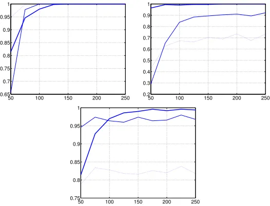
Figure 1: Probability of correct identification as a function of series length. Thick line: our method; continuous thin line: Johansen test withα=0.01; dotted line: Johansen test withα=0.05. Dimensionn=2 and series simulated according to (11) with (from top to bottom and from left to right)r=2 (the series are actually stationary),r=1 (cointegrated) andr=0 (no cointegration).

Within this boundary, determining the SF is equivalent to determining the coin-tegration rank, so we can actually compare the probability of correctly identifying the cointegration rank with the Johansen test and with our procedure. We estimate both probabilities counting for each series lengthT how many times both methods get it right. In Figure 1 and Figure 2, we represent the length-dependent curves for dimensions 2 and 3.

Both in dimension 2 and 3, our method seems to do very well in the nontrivial cases when 0<r<n, clearly outperforming the Johansen test, particularly in

0 100 200 300 400 500 0.65

0.7 0.75 0.8 0.85 0.9 0.95 1

0 100 200 300 400 500 0

0.2 0.4 0.6 0.8 1

0 100 200 300 400 500 0

0.2 0.4 0.6 0.8 1

0 100 200 300 400 500 0.5

0.6 0.7 0.8 0.9 1

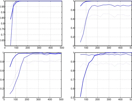
Figure 2: Probability of correct identification as a function of series length. Thick line: our method; continuous thin line: Johansen test withα=0.01; dotted line: Johansen test withα=0.05. Dimensionn=3 and series simulated according to (11) with (from top to bottom and from left to right)r=3 (the series are actually stationary),r=2 (cointegrated with rank 2),r=1 (cointegrated with rank 1) andr=0 (no cointegration).

the probability of correct identification with our method grows at a slower pace, it always starts at pretty decent levels for very short series, unlike the Johansen test, which yields very small probabilities in some cases.

4.2 Results in theI(2)case

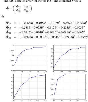
Now, we consider cases with

d(z) = (1−z)2; DΨ(z) =





Ir0 0 0

0 (1−z)Ir1 0

0 0 (1−z)2_I

n−r0−r1 

. (12)

Additionally, we also try a case with negative unit roots that can be interpreted as biannual seasonality, that is,

d(z) =1−z2; DΨ(z) =

Ir 0

0 (1−z2)In−r

. (13)

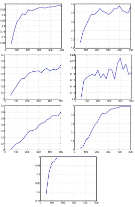
In Figure 3, we see that the convergence is somewhat slower in some cases, in particular whenr0=r1=1, but we got fairly good probabilities for long series, above 150 observations length. In Figure 4 forn=3 we have some cases that are really tough. Since the convergence is slower, we represent the curves with the length parameter going up to 500 observations. In particular, the convergence of the caser0=2,r1=0, seems to be very slow. It is not surprising that forn=3 is more difficult to identify correctly the case, since there are much more possible cases to distinguish. In fact, considering only roots equal to unity, the number of combinations forn−dimensionalI(d)series grows as(d+1)n−1_{. However, we} see that the seasonal case works pretty well even for relatively short series.

5 Real data example

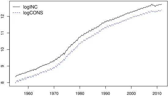
To illustrate the use of the method and the package GVEC, we will identify a model for a data set similar to the one used in Hylleberg et al. (1990). In particular,y1_t

The AIC-selected order for the var is 5. The estimated VAR is

ˆ

Φ=

Φ₁₁ Φ₁₂ Φ₂₁ Φ₂₂

with

ˆ

Φ₁₁ = 1−0.400B−0.105B2−0.107B3−0.462B4+0.129B5

ˆ

Φ₁₂ = −0.588B+0.073B2+0.112B3−0.254B4+0.603B5

ˆ

Φ_{21 = −0.021B+0.014B}2_−0.108B3_+0.091B4_−0.056B5 ˆ

Φ₂₂ = 1−0.908B−0.000B2+0.0646B3−0.973B4+0.899B5.

50 100 150 200 250

0.75 0.8 0.85 0.9 0.95 1

50 100 150 200 250

0.4 0.5 0.6 0.7 0.8 0.9 1

50 100 150 200 250

0.4 0.5 0.6 0.7 0.8 0.9 1

50 100 150 200 250

0.9 0.92 0.94 0.96 0.98 1

0 100 200 300 400 500

1960 1970 1980 1990 2000 2010

8

9

10

11

12

logINC logCONS

Figure 5:Logarithm of Income and Consumption of the UK.

We apply the automatic method withεT=T−1/3and get the matrix diag(d1,d2) withd1=1−Bandd2= (1−B)(1−B4), or

∇ ₀

0 ∇·∇_s

,

where∇=1−Band∇_s=1−Bs. Then, the GVEC is

Γ(B)∇_s·∇yt =Π0(1,1)∇syt−1+

Π(₀1_,1,−)+Π(₀1_,1,+)B

(1−B2)∇yt−1+

Π(₂1)

,1(1−B−B2+B3)∇yt−1+εt.

whereΓ(B)has orderp=4 and the interceptµ equals to(−0.00369,−0.00343)′

and

Π(₀1_,1)=

−0.185 0.139

−0.717 0.667

Π(₁1_,1,−)=

−0.046 0.023

−0.090 0.104

Π(₁1,+)

,1 =

−0.020 0.038 0.190 −0.069

Π(₂1)

,1=

0.032 0.001 0.070 −0.019

.

this means that according to our method both series are I(2) with respect to frequency zero andI(1)with respect to the seasonal frequencies. In this respect, this is consistent with the univariate results obtained with TRAMO/SEATS. The model identified is equivalent to a seasonal VEC model as the one analyzed in HEGY for the first differences. Therefore, the interpretation of the coefficients in the HEGY model applies here. For example, by extracting the eigenvector corresponding to the greatest eigenvalue ofΠ(₀1_,1), we get that there is cointegration in the with respect to frequency zero and the cointegrating vector is quite close to

(1,−1).

6 Conclusions

We have tried to unify the treatment of cointegration for practitioners, in doing so we have contributed in providing unified theoretic framework for a broad class of situations. To this end we have provided a theoretical framework that covers any process that can be represented by an autoregressive model with unit roots. Our ap-proach covers I(1), I(2), multicointegration, polynomial and seasonal cointegration. From the practioner perspective we put forward an automatic method to identify GVEC models based on an estimate of the Smith Forms of the autoregressive model. Our method is competitive with Johansen test, in the restricted cases in which the latter applies, with the advantage that the new method can cope with other practical situations.

Further research can be conducted to extend the theoretical framework to fractional integration or other forms of long memory and to relax some assumptions such as the rationality of the transfer function. Also, in order to apply these ideas to large dimension, or even to panel data, the algorithms need to be adapted, since in their actual form they are only suited to moderate dimensions.

Acknowledgements: Mariano Matilla-García is grateful to the following research grants:

FEDER funds, and to the program of Groups of Excellence of the Región de Murcia, the Fundación Séneca , Science and Technology Agency of the Región de Murcia, project 19884/GERM/15.

A Appendix

Proof of Proposition 1. First, the ranksrk,j are uniquely determined because rk,j=dimCnha(ω_k):a(B)′y_t∼I(d_k−j)i.

By the uniqueness of the ranks, it suffices to prove that for every processyt,Ψ

can be represented as in (a) and then, there are exactlyn−∑_ℓ≥jsk,ℓcointegration

vectors whose values atωk are linearly independent.

The first step is a consequence of Proposition 2.11 from Hungerford (1980), applied to the ringR={f/g:∀k,g(ωk)6=0}. We have then a representation

Ψ(z) =U(z)DΨ(z)V(z), where the elements of the diagonal ofDΨ(z)divide one each otherdi,i(z)|di+1,i+1(z). This allows to representyt as

d(B)yt=U(B)DΨ(B)V(B)εt. (14)

It is clear that we can factorizeDΨ(z) asDΨ(z) =D0(z)·. . .·Dg(z). If we

focus on a certaink, all the other unit roots can be moved to the left or the right so we can writeΨ(z) =Uk(z)Dk(z)Vk(z). where detU(ωk),detV(ωk)6=0. If we

chooseG(z)as the lastrk,j rows ofUk(z)−1, then we get G(B)yt = [01×n−rk,j :. . .]d(B)

−1_D

k(B)Vk(B))εt.

Since the lastrk,jelements of the diagonal ofDΨ(z)are divided by(1−ωk−1z)j, we

get thatG(B)yt ∼Ik(dk−j). On the other hand,G(ωk)is full rank for otherwise Uk(z)would have a root atωk, which is contradictory with the conditions of the SF.

Thus, there are at leastr′_k,j:=n−∑_ℓ≥jsk,ℓcointegrating vectorsa(z)∈A such

that{a(ωk)}a∈A are linearly independent. Hencer_k,j ≥r′_k,j. To see that this is actually an identity, let us assume thatrk,j>r′k,j. Then, we arrange the cointegration

letA2 be a(n−rk,j)×nconstant matrixA2 such that[A1(ωk)′:A′2]is invertible to remain in the RHS of the representation, somhas unit roots.

Lemma 1. The ring of polynomialsC[z]and R={f/g:f,g∈C[z],∀k,g(ωk)6=0} are PIDs.

Proof. Every Euclidean ring is a PID (see Hungerford, 1980, theorem 3.9). The fact thatC[z]is an Euclidean ring is elementary. We will prove that forR. We can write any f/g∈Ras f =hk/g, wherehhas roots only among{ωℓ}s_ℓ−₌10andkhas none there. Then, if we denote by∂pthe degree of polynomialp, we can define ϕ(f) =∂h. To divide f1=h1k1/g1by f2=h2k2/g2, we first divideh1byh2, so h1=qh2+r. Then f1= (qh2+r)k1=qh2k1/g1+rk1/g1=q f˜ 2+rk1/g1, where

˜

q= (g2k1g₁−1k−₂1)qandϕ(rk1/g1) =∂r<∂h2=ϕ(f2).

Proof. Letqk,ℓ(z) =p(z)/(z−θk)ℓ. Is is easy to see that there areck,ℓ∈Csuch

that at eachθk,∑k∑mℓ=k1ck,ℓqk,ℓ(z)and its derivatives up tomk−1 coincide with f(z). It suffices to write down the identities and see that they form a triangular linear system.

Let nowqk,ℓ,0(z) = p(z)/(z2−2Reθk+|θk|2)ℓ andqk,ℓ,1(z) =qk,ℓ,0(z)z. We will see thatB_{={qk,ℓ: Imθk =0} ∪ {qk,ℓ,0,qk,ℓ,1: Imθk>0}are linearly} inde-pendent inV, the space of the polynomials of degree up to∂p−1. Let us assume that there is a linear combination of the elements ofB_{that equals zero. Then,}

∑

Now, we can integrate the last identity along a closed path encircling only θk. By the Residue Theorem (Rudin, 1987), for real θk we obtain that

2πick,ℓ/θk=0, whereas for a pair of conjugate roots, we get 2πck,ℓ,0/(θk2Imθk) +

2πck,ℓ,1/(2Imθk) =0 and−2πck,ℓ,0/(θ¯k2Imθk)−2πck,ℓ,1/(2Imθk) =0.

Conse-quently,ck,ℓ,0=ck,ℓ,1=0. Since the number of elements inBequals the dimension ofV, they form a basis.

To see that the coefficients are real, notice that the left hand side of (15) equals

The-On the other hand, let us writeδj+1=cjδj. We can dividec1betweenz. We

We can repeat this device to obtain the form

A(rh−1)(z)δh(z) +

The last step consists of rewriting the terms of the last sum in (17). We divide the elements ofB(₁1)(z)byc1(z)using lemma 2, so we getB₁(1)(z) =c1(z)Q1(z)+R1(z), whereR1(z)is a polynomial matrix whose elements have the form given by lemma 2. Then, ifc1has rootsθkwith multiplicitiesmk, then

We will prove first the case when all unit roots are equal to 1. Then, existsr,ssuch thatδ1= (1−z)sandδh= (1−z)r. We will write∆i(z) = (1−z)i. Let us define

We will write down the form of the least squares estimator. Then by defining

means of the Beveridge-Nelson decomposition we can representYt in a similar

× (T

We will sketch now the proof for the general case. In order to make the notation less cumbersome, we denote the multi-index(j,k, ℓ)asα. We consider its values ordered with the lexicographical order. Then, y(_tα)=∆_α(B)yt. Now,

Let us denotezν,τ,t=Lν,τ(B)yt= (1−θτ−1z)−νC(B)εt. When 0<τ<b,zν,τ,t

andzν,s−τ,t are conjugate. We can also make a transformation similar to that in

section 3 of TT to transform the conjugate pairs into pairs of real and imaginary parts w₍uν,τ,t =ν,τ,t,vν,τ,t)′. Then, there is an invertible matrix P such that

We can deal now with theW’s andC’s in a similar fashion as the unity case, along the lines of section 4 of TT.

Proof of Proposition 4. It suffices to see that the algorithm described in annex B (i) can be described as (5)-(6) withε=0, (ii) it stops and (iii) when it stops, the state variableDis the Smith form ofA.

The first assertion can be proved as follows: let the state variable ek

com-prise all the flags, an additional flag indicating whether r=0 and the current line number. Then, all the actions in the algorithm are either (a) control flow sentences and changes ofr, that are (5) or (b)admissible operations, that are (6). Thus, we can write a meta-algorithm that runs over the algorithm of the annex as follows:

3: ifsentence(nline)is type (a)then

4: performek= f0(ek−1,A(k−1)) 5: else

6: performA(k)=g(ek−1,A(k−1))andnline←nline+1 7: end if

8: k←k+1 9: end loop

In order to see that the algorithm always stops and that when it stops, we get the Smith form, we can easily adapt the proof in Hungerford (1980), page 340, replacing the arguments based on the finiteness of the divisors of an element in the ring, by the fact that the degree function takes values inNand thus it can decrease only a finite number of times.

Proof of Theorem 1. To simplify the proof, we assume that the algorithm does not involve the conditionr=0, but just conditions of the formai j=0. The proof can

be easily adapted then by considering an augmented matrix ˜A= [A:R], where

R= (ri j)i jandri j is the remainder of the Euclidean division ofaiiandai j.

We will denote by(ek,A(k))the pair we obtain as the result of iterating (5)-(6)

starting fromA, whereas(eˆk,Aˆ(k))is got by iterating theε−approximate version

of (5)-(6) starting from ˆA. We will see that∀k,

P[eˆℓ=eℓ,∀ℓ≤k]→1 (18)

ˆ

A(k)−A(k)=wk_T, (19) where∀δ>0,∃M>0,T0such that∀T≥T0,P[ξT−1kwkTk>M|eˆℓ=eℓ,∀ℓ≤k]<δ.

For any random variable that satisfies this property ofwk_T, we writeOcp(ξT), that

is,conditional orderξT in probability. It is easy to see that this property behaves

in a similar fashion to the usual order in probability, in particular, the product of twoOcp(ξT)andOcp(ηT)sequences isOcp(ξTηT).

First, we will see that P[eˆℓ =eℓ,∀ℓ≤k]→1. Letiand jbe indexes such

that given ˆek−1=ek−1, fεT takes a certain valueα if|aˆ

(k−1)

i j |<ε and a valueβ if |aˆ(_{i j}k−1)| ≥ε. We will use that

Peˆℓ=eℓ,∀ℓ≤k=Peˆk=ek|eˆℓ=eℓ,∀ℓ≤k−1Peˆℓ=eℓ,∀ℓ≤k−1.(20)

There are two cases, eithera(_{i j}k−1)=0 ora_{i j}(k−1)6=0. Ifa(_{i j}k−1)=0, then

Peˆℓ=eℓ,∀ℓ≤k=P|aˆ(i jk−1)| ≤εT|eˆℓ=eℓ,∀ℓ≤k−1Peˆℓ=ev,∀ℓ≤k−1

From (18) andξ_T−1εT −→∞, it follows,

P|aˆ(_{i j}k−1)| ≤εT|eˆℓ=eℓ,∀ℓ≤k−1

= (21)

Pξ−1

T |aˆ

(k−1)

i j −a

(k−1)

i j | ≤ξT−1εT|eˆℓ=eℓ,∀ℓ≤k−1→1.

Let us now consider the case thata(_{i j}k−1)6=0. Then,

P|aˆ(_{i j}k−1)| ≤εT|eˆℓ=eℓ,∀ℓ≤k−1

= (22)

P|aˆ(_{i j}k−1)−a_{i j}(k−1)| ≤εT|eˆℓ=eℓ,∀ℓ≤k−1

→1,

because|aˆ(_{i j}k−1)−a_{i j}(k−1)| → |a(_{i j}k−1)|>0 in probability andεT→0.

Consequently, (18) is proved. Let us see (19). We denote by ˆS(k−1) and

S(k−1)the matrices of the admissible operation (d) performed on ˆA(k−1)andA(k−1)

respectively. Then,

ˆ

A(k)−A(k)=Aˆ(k−1)Sˆ(k−1)−A(k−1)S(k−1)= (23)

=h_Aˆ(k−1)_−A(k−1)i_Sˆ(k−1)_+A(k−1)h_Sˆ(k−1)_−S(k−1)i_{. (24)}

For row operations, we find a similar identity. Thus, we just need to prove that ˆ

S(k−1)−S(k−1)=Ocp(ξT)and use that in turn, this implies ˆS(k−1)=Ocp(1).

and its counterpartcfromA(k−1). The degrees of the ˆa(_{i j}k)are bounded conditionally to ˆeℓ=eℓ,∀ℓ≤k, so we can use assumption 4 and

ˆ

a_ii(k−1)−a_ii(k−1)=Ocp(ξT) (25)

ˆ

a_{i j}(k−1)−a_{i j}(k−1)=Ocp(ξT), (26)

and get that ˆc−c=Ocp(ξT)and thus ˆS(k−1)−S(k−1)=Ocp(ξT).

The case of the admissible operations (c) and (e) are similar, while (a) and (b) are isometries and thus they satisfy trivially the condition.

Lemma 3. The Euclidean division and the mapping u are continuous in R=R[z].

Proof. Ifδ <1, then|q−q′|<δ entailsϕ(q′) =ϕ(q). Thus, the degrees of the polynomials, and consequently the number of operations involved in the division are bounded. Since the algorithm only requires addition, multiplication and division by the lead coefficient of the divisor, the continuity is granted.

The mappinguin this case boils down to calculate the inverse of the leading coefficient of the argument and by definition, the leading coefficient is always nonzero.

Before proving Proposition 5, we need some preliminary results. In TT, it is proved that for purely nonstationary processes, that is, processes that satisfy a

A(B)yt =M(B)εt such that detΦ(z)has only unit roots, the autoregressive least

squares estimates are consistent. For processes that are nonstationary, but not purely nonstationary, that is, when detA(z)has roots on and outside the unit circle, the purely nonstationary part of the estimates (in some sense that is specified in the proof of proposition 5) is consistent.

We will prove that ˜S(A,0;R[z]) does not depend on the stationary part and that ˆΦ→A∗such that the ˜S(A∗,0;R[z]) =S˜(A,0;R[z])and thus ˜S(Φˆ,εt;R[z])

p →

˜

S(A,0;R[z]).

Now, we see that if we can decompose the autoregressive polynomial into stable and purely unstable components, only the purely unstable component determines

˜

S(A,0;R1(z)).

Lemma 4. Let Φ_s(z) be stable (i.e., without unit roots). Then, for anyΦ_n(z), possibly with unit roots,S₍₍Φ−1

Proof. For ease of notation, we drop the superscript ·Φ_{. Let Φ}

n=U DV and (Φ−1

n +Φ−s1)−1 = Θ−1Φ, where Φ and Θ are left-coprime. Then Θ−1Φ =

h

DVadjΦ_{sdetU+adjUdet}Φ_si−1_·h_DVdetΦ_sdetUi_{. By theorem 2.1.1 in} Han-nan and Deistler (1988), we know that there exists some unimodular matrixCsuch thatΦ=CDVdetΦ_sdetU. Therefore(Φ−1

n +Φ−s1)−1=Θ−1CDVdetΦsdetUand

thus, its SF isD.

Proof of Proposition 5. We will use the representationYt=FYt−1+at, whereYt= (y′_t, . . . ,y_t′_−p+1)′_,a

t =LΘ(B)εt,Fis the companion matrix ofΦandLcomprises

the first n columns of Inp. Let J=PFP−1 be the Jordan form of F. We can

decompose it in the stable and non-stable parts asJ=diag(Js,Jn).

If we callUt=PYt, thenUt = (Ust,Unt)′, whereUst andUnt are the stable and

unstable components. In TT it is proved that ˆJs→Js∗and ˆJn→Jn, whereJs∗6=Js

whenΘ6=0, but we can see thatJ_s∗is stable, that is, it has all its eigenvalues inside the unit disk. SinceUst is stable,Ust=∑k≥0Ψkεt−k, with∑kkΨkk2<+∞. Then, J_s∗=Γ(0)−1_{Γ(1), whereΓ(0) =∑}

k≥0ΨkΨ′kandΓ(1) =∑k≥0Ψk+1Ψ′k.

Let us see that all eigenvalues ofJ_s∗have modulus less than one. Letube an eigenvector andλits eigenvalue, soΓ(1)u=λΓ(0)uand thenu′Γ(1)u=λu′Γ(0)u. Let us consider the infinite sequences x= (x0,x1, . . .), wherexj∈Rn endowed

with the scalar producthx,yi=∑_kx′_kyk. Then, by defininga= (Ψ′0u,Ψ′1u, . . .)and b= (Ψ′₁u,Ψ′₂u. . .), thenu′Γ(0)u=ha,aiandu′Γ(1)u=ha,bi. Sincekbk ≤ kak, we conclude that|λ|<1 unlessaandbare linearly dependent, but his implies that Ψ′

ku=αkw. Then,α=λand necessarily|α|<1 becauseΨkis square-summable.

We can recover the infinite MA representation of yt as yt =L′P−1(1− JB)−1_PLε

t. SinceJ=diag(Js,Jn), then

ˆ

Φ(z)−1→L′P−1

(1−J_s∗B)−1 ₀

0 0

PL+L′P−1

0 0

0 (1−JnB)−1

PL

B Algorithm

For a ∈ R, T_{i j}a is the unitary matrix that multiplied on the right side adds the ith column to the jth one, whereas matrix Si j swaps columns i and

j.

1: fori=0 ton−1do 2: for j=0 tondo 3: Ai j←u(Aii)Ai j

4: end for

5: f lagdiv←T RU E

6: while f lagdiv do

7: f lagz←T RU E

8: while f lagzdo

9: f lagrow←T RU E

10: while f lagrowdo

11: MAKE ROW ZEROS

12: end while

13: f lagcol←T RU E

14: while f lagcoldo

15: MAKE COLUMN ZEROS

16: end while

17: f lagz←FALSE

18: for j=i+1 tondo

19: ifAi j6=0 orAji6=0then

20: f lagz←T RU E

21: end if

22: end for

23: end while

24: BOX DIVISIBILITY

25: end while 26: end for

SUBALGORITHM MAKE ROW ZEROS.

2: for j=i+1, . . . ,ndo

3: ifAi j6=0then

4: nzcount ←nzcount+1

5: r←remainder from (Ai j=Aiiq+r)

6: ifr=0then

7: q←quotient from (Ai j=Aiiq+r)

8: A←AT_{i j}q

9: U←(T_{i j}q)−1_U

10: else

11: q←quotient from (Ai j=Aiiq+r)

12: A←AT_{i j}qSi j

13: U←S−_{i j}1(T_{i j}q)−1_U

14: end if

15: end if 16: end for

17: ifnzcount=0then 18: f lagrow←FALSE

19: end if

SUBALGORITHM MAKE COLUMN ZEROS

1: nzcount←0 2: for j=i+1 tondo 3: ifAji6=0then

4: nzcount ←nzcount+1

5: r←remainder from (Ai j=Aiiq+r)

6: ifkrk<εthen

7: q←quotient from (Ai j=Aiiq+r)

8: D←T_{i j}q(q)A

9: V ←V(T_{i j}q)−1

10: else

11: q←quotient from (Ai j=Aiiq+r)

12: A←Si jTi jqA

13: U←U(T_{i j}q)−1_(S

i j)−1

15: end if

16: end for

17: ifnzcount=0then 18: f lagcol←FALSE

19: end if

SUBALGORITHM BOX DIVISIBILITY

1: f lagdiv←FALSE

2: for j=i+1 tondo 3: fork=i+1 tondo

4: r←remainder from (Aik=Aiiq+r)

5: ifr6=0then 6: f lagdiv←T RU E

7: D←Si jA

8: V ←V S−_{i j}1

9: break for

10: end if

11: end for

12: if f lagdiv=T RU Ethen

References

Barrio Castro, T., and Osborn, D. (2011). HEGY Tests in the presence of moving averages. Oxford Bulletin of Economics and Statistics, 73: 691–704. URL

http://onlinelibrary.wiley.com/doi/10.1111/j.1468-0084.2011.00633.x/abstract.

Engle, R., and Granger, C. (1987). Co-integration and error correction: Rep-resentation, estimation and testing. Econometrica, 55: 251–76. URL http:

//www.jstor.org/stable/1913236.

Franchi, M. (2006). A general representation theorem for integrated vector autore-gressive processes. Discussion paper 06-16, University of Copenhagen. URL

http://www.economics.ku.dk/research/publications/wp/2006/0616.pdf/.

Franchi, M. (2007). The integration order of vector autoregressive processes.

Econometric Theory, 23: 546–553. URLhttp://www.jstor.org/stable/4497802.

Granger, C. (1981). Some properties of time series data and their use in econometric model specification. Journal of Econometrics, 23: 121–130. URLhttp://www.

sciencedirect.com/science/article/pii/0304407681900798.

Granger, C. W., and Joyeux, R. (1980). An introduction to long-memory time series models and fractional differencing. Journal of time series analysis, 1: 15–29.

URLhttp://onlinelibrary.wiley.com/doi/10.1111/j.1467-9892.1980.tb00297.x/

abstract.

Granger, C. W. J., and Lee, T. (1989). Investigation of production, sales and inventory relations using multicointegration and non-symmetric error correction models. Journal of Applied Econometrics, 4 (S1): S145–S159. URL http:

//onlinelibrary.wiley.com/doi/10.1002/jae.3950040508/abstract.

Haldrup, N., and Salmon, M. (1998). Representations of I(2) Cointegrated Systems Using the Smith-McMillan Form. Journal of Econometrics, 84: 303–325. URL

http://www.sciencedirect.com/science/article/pii/S0304407697000882.

Hungerford, T. W. (1980). Algebra. Springer, New-York.

Hylleberg, S., Engle, R. F., Granger, C. W. J., and Yoo, B. S. (1990). Seasonal integration and cointegration. Journal of Econometrics, 44: 215–238. URL

http://www.sciencedirect.com/science/article/pii/030440769090080D.

Ing, C.-K., Sin, C., and Yu, S.-H. (2007). Efficient selection of the order of an AR(∞_{): a unified approach without knowing the order of integratedness.} Discussion paper, Institute of Statistical Science, Academia Sinica.

Johansen, S. (1988). Statistical analysis of cointegration vectors. Journal of Economic Dynamics and Control, 12: 231–254.URLhttp://www.sciencedirect.

com/science/article/pii/0165188988900413.

Johansen, S. (1992). A representation of vector autoregressive processes integrated of order 2. Econometric Theory, 8: 188–202. URLhttp://www.jstor.org/stable/

3532439.

Johansen, S., and Juselius, K. (1990). Maximum likelihood estimation and in-ference on cointegration with applications to the demand for money. Oxford Bulletin of Economics and Statistics, 52: 169–210. URL http://onlinelibrary.

wiley.com/doi/10.1111/j.1468-0084.1990.mp52002003.x/abstract.

Levin, A., and Lin, C. F. (1993). Unit root tests in panel data: Asymptotic and finite-sample properties. Discussion paper, University of California, San Diego.

Levin, A., Lin, C. F., and Chu, C. S. J. (2002). Unit root tests in panel data: Asymptotic and finite-sample properties. Journal of Econometrics, 108: 1–24.

URLhttp://www.sciencedirect.com/science/article/pii/S0304407601000987.

Lewis, R., and Reinsel, G. C. (1985). Prediction of multivariate time series by autoregressive model fitting. Journal of Multivariate Analysis, 16: 393–411.

URLhttp://www.sciencedirect.com/science/article/pii/0047259X85900272.

Ling, S., and Li, W. K. (1998). Limiting distributions of maximum likelihood estimators for unstable autoregressive moving-average time series with general autoregressive heteroscedastic errors. The Annals of Statistics, 26: 84–125. URL

Maravall, A. (2008). Notes on programs TRAMO and SEATS. Discussion paper, Bank of Spain. URL http://www.bde.es/f/webbde/SES/servicio/ Programas_estadisticos_y_econometricos/Notas_introductorias_TRAMO_

SEATS/ficheros/Part_III_Seats.pdf.

Paruolo, P. (1996). On the determination of integration indices in I(2) systems.

Journal of Econometrics, 72: 313–356. URL http://www.sciencedirect.com/

science/article/pii/0304407695017259.

Rudin, W. (1987). Real and complex analysis. McGraw-Hill, New York.

Tsay, R. S., and Tiao, G. C. (1990). Asymptotic properties of multivariate nonsta-tionary processes with applications to autoregressions. The Annals of Statistics, 18: 220–250. URLhttp://www.jstor.org/stable/2241542.

Worthington, A. C., and Higgs, H. (2010). Assessing financial integration in the European Union equity markets: Panel unit root and multivariate cointegration and causality evidence. Journal of Economic Integration, pages 457–479. URL

http://www.jstor.org/stable/23000868.

Yap, S. F., and Reinsel, G. C. (1995). Estimation and testing for unit roots in a partially nonstationary vector autoregressive moving average model. Journal of the American Statistical Association, 90: 253–267. URLhttp://www.jstor.org/

stable/2291150.

Yu, J., and Lee, L. (2010). Estimation of unit root spatial dynamic panel data models. Econometric Theory, 26: 1332–1362. URLhttp://www.jstor.org/stable/

Please note:

You are most sincerely encouraged to participate in the open assessment of this article. You can do so by posting comments.

Please go to:

http://dx.doi.org/10.5018/economics-ejournal.ja.2016-26

The Editor