MAPPING ALPINE VEGETATION LOCATION PROPERTIES BY DENSE MATCHING
Robert Niederheiser a, *, Martin Rutzinger a, Andrea Lamprecht b, Klaus Steinbauer b, Manuela Winkler b, Harald Pauli b
a Institute for Interdisciplinary Mountain Research - Austrian Academy of Sciences, Innsbruck, Austria -
(robert.niederheiser, martin.rutzinger)@oeaw.ac.at
b GLORIA, Austrian Academy of Sciences and University of Natural Resources and Life Sciences, Vienna, Austria
KEY WORDS: Vegetation, close-range photogrammetry, structure from motion, dense matching, mountain research, MicMac, GLORIA
ABSTRACT:
Highly accurate 3D micro topographic mapping in mountain research demands for light equipment and low cost solutions. Recent developments in structure from motion and dense matching techniques provide promising tools for such applications. In the following, the feasibility of terrestrial photogrammetry for mapping topographic location properties of sparsely vegetated areas in selected European mountain regions is investigated. Changes in species composition at alpine vegetation locations are indicators of climate change consequences, such as the pronounced rise of average temperatures in mountains compared to the global average. Better understanding of climate change effects on plants demand for investigations on a micro-topographic scale. We use professional and consumer grade digital single-lens reflex cameras mapping 288 plots each 3 x 3 m on 18 summits in the Alps and Mediterranean Mountains within the GLORIA (GLobal Observation Research Initiative in Alpine environments) network. Image matching tests result in accuracies that are in the order of millimetres in the XY-plane and below 0.5 mm in Z-direction at the second image pyramid level. Reconstructing vegetation proves to be a challenge due to its fine and small structured architecture and its permanent movement by wind during image acquisition, which is omnipresent on mountain summits. The produced 3D point clouds are gridded to 6 mm resolution from which topographic parameters such as slope, aspect and roughness are derived. At a later project stage these parameters will be statistically linked to botanical reference data in order to conclude on relations between specific location properties and species compositions.
* Corresponding author
1. INTRODUCTION
Vegetation on mountain summits is under pressure. Due to rising temperatures in mountain areas there is a change in species composition on mountain summits. Research has shown that species are shifting towards higher altitudes, which leads to an increase in species richness on boreal and temperate summits, whereas there is a species-loss on Mediterranean summits (Pauli et al. 2012). High-elevation species, endemics in particular, are put under pressure by the rising temperature and through increasing competition. In consequence, species that are not able to adapt or to migrate may go extinct, at least locally. However, steep elevation gradients and fine-grained roughness of terrain, especially, may present refugia for cryophylic vegetation and mitigate the effects of rising temperatures (Scherrer & Körner 2010).
It has also been proposed that these changes in species richness are predetermined by geomorphological i.e. topographic factors such as aspect and slope (Scherrer & Körner 2011). In order to quantify these factors high-detailed digital terrain models (DTMs) are required. However, freely available elevation models such as Shuttle Radar Topography Mission (SRTM) or the European digital elevation model (EU-DEM) offer only a coarse representation of local topography at roughly 30 m resolution (EEA 2016, USGS 2016). These models are not detailed enough for small-scale and micro-topographic analysis. European national agencies provide digital elevation models (DEMs) that are based on aerial laser scanning (ALS) at finer
resolutions, such as the DEM provided by the Austrian county Steiermark at 10 m resolution (GIS-Steiermark 2016), the Spanish DEM at 5 m resolution (Instituto Geográfico Nacional 2016), or the DEM of the Italian province Trentino at 1 m resolution (Ufficio Sistemi Informativi - Servizio autorizzazioni e valutazioni ambientali 2016).
Operational surveying techniques such as topographic light detection and ranging (LiDAR) from airborne or terrestrial platforms are very costly and require for a lot of heavy equipment. Unmanned Aerial Vehicles (UAVs) are strongly effected by weather, i.e. wind conditions. In general, mountain summits are often not accessible enough for making use of these techniques. However, recent developments in close-range photogrammetry applying Structure-from-Motion (SfM) and dense-matching techniques offer new possibilities of mapping high-detail morphological traits in alpine terrain.
This paper is structured as follows. Section 1 introduces the overall research framework. The elaborated workflow for data acquisition and processing considering methods and materials are described in Section 2. Section 3 presents the results, which are discussed in Section 4. Section 5 gives an outlook of follow-up work we have planned.
2. METHODS AND MATERIALS
This section presents the study region (Sect. 2.1) and describes the image acquisition process (Sect. 2.2). Then, a general description of the applied SfM workflow follows (Sect. 2.3).
2.1 Study regions
Test sites are distributed throughout the Alps and Mediterranean Mountains as two bioms with different climate characteristics. Three GLORIA regions were selected in the Mediterranean mountains and in the Alps, representing the large-scale elevation gradients and the lower alpine, upper alpine and sub-nival ecotones, respectively (Figure 1 and Figure 2).
Figure 1. Overview of test regions in the Alps and the Mediterranean mountains (Basemap: MaqQuest)
Each GLORIA region is composed of four summits, representing the regional elevation gradient from the treeline to the sub-nival ecotone (see Pauli et al. 2015). For this study, in each region only the three higher summits per region were investigated. The lowest summits are situated in the treeline ecotone and therefore, especially in the Alps, are fully covered with vegetation which makes them unsuitable for the applied method.
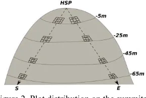
For each summit 16 plots with a size of 3x3 m are mapped, which results in a sampling of 288 plots, in total. The local elevation gradients of the single summits are represented by placing the plots at specific elevations, 5 m, 25 m, 45 m and 65 m below the highest summit points (HSP) in all four cardinal directions (Figure 2). The exact plot locations are determined in the field in order to select representative sites that represent the local ecosystem. The results presented in Section 3 refer to one selected study region, the Hochschwab in the North-Eastern Alps (Austria).
2.2 Image acquisition and setup
For the later SfM and dense matching processing up to 300 images are captured per plot in a semi-structured manner. Considering vegetation cover, height and density, each plot is evaluated in the field if creating dens point clouds using terrestrial photogrammetry is feasible. If the vegetation cover is
too high or too few ground patches are visible only overview images and a few vertical images are captured for documentation purposes and qualitative interpretation.
Figure 2. Plot distribution on the summits
Vertical images of the plots are captured using a pole with a digital single-lens reflex (DSLR) camera attached held at approximately two metres height above the plots (Figure 3). Doing so, a flight path over the plot is simulated. Oblique images at three different incident angles from two different distances are captured by walking around the plot. Combining the vertical and oblique images a dome structure of camera positions around and above the plots is created minimizing possible occlusions and shadowing effects by rocks and rough terrain.
Figure 3. Image collection in the field with a camera attached to an extendable pole. In the foreground a target cube and wooden
ruler
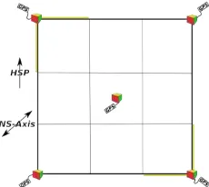
We place five well-defined targets in and next to the plots in order to be able to scale and orient the derived 3D point clouds and DEMs respectively (Figure 4). The targets are wooden cubes with 9.5 cm edge length. The faces of the cubes are colour-coded and equipped with compasses and miniature levellers. Hence, in the field we are able to place the cubes in an oriented manner, always facing north with a designated side-face, and levelled horizontally. We also place two foldable rulers with a distinct coloration next to the plots. By combining the known absolute measurements of the cubes and the rulers we can scale, orient and therefore evaluate the resulting terrain models form the SfM workflow.
The cubes are also equipped with low-cost GPS loggers. During the surveying of the plots these GPS loggers continuously record their positions yielding positional point clouds for a rough estimation of the absolute positions.
Figure 4. Schematic of plot setup with colour coded cubes and wooden rulers (yellow).
2.3 Processing Workflow
The point cloud processing is done using a combination of different software packages. First, the open-source software MicMac (2016) is used to compute the raw point clouds. Second, the open-source software CloudCompare (2015) is used to merge and clean the multiple point clouds that MicMac produces. Third, GRASS GIS (2016) and R (2015) are used for statistical calculations on the gridded point clouds on a per-plot basis and for comparisons on a regional scale.
An optimized SfM approach is very labour intensive. First, images need to be selected carefully supporting a successful matching and point cloud generation. Several parameters in the MicMac workflow would require optimization to fit the individual scene characteristics. Such parameters are for example regularization parameters, the selection of a regularization algorithm itself and the neighbourhood definition, and parameters for correlation coefficients. Furthermore, some scenes have sharper edges than others (such as large blocks on a steep slope) or have a more homogeneous texture, such as grass, for which such optimizations could be applied. Finally, the point cloud needs to be scaled and oriented manually. However, in operational processing, i.e. handling a large number of plots and the resulting number of point clouds in a feasible manner, not all parameters can be optimized considering all local conditions. Therefore, - as described in the following - a standard approach has been developed and applied to all plots minimizing manual input wherever possible and reasonable.
In a first iteration only vertical images are used. After choosing the relevant images tie-points between all image pairs are calculated facilitating the SIFT++ algorithm (Institut national de l’information géographique et forestière 2016). Based on those tie-points a self-calibration is done and the inner and outer orientation of the sensor is computed. The resulting arbitrary coordinate system is then transformed into metric scale by selecting the corner pixels of the centre cube in a small number of images and giving them real relative distance coordinates around a centre point (0,0,0). The dense-matching for specific master images is done on the transformed sparse point cloud. If a plot is very steep or includes large objects such as boulders oblique images are selected carefully so that side faces are represented in the point cloud as well. The image matching is then started again.
As a final step dense point clouds are exported and further processed with CloudCompare. All point clouds of a single plot resulting from the different master images are loaded and merged. A subsampling is applied by an octree level of 10 removing duplicate points. Statistical outliers are removed considering the 15 nearest neighbours and rejecting points that are farther away than their average distance plus one standard deviation (CloudCompare Wiki, 2015). Finally, the point clouds are georeferenced in a world coordinate system. Further analysis and the derivation of parameters, such as roughness, slope or aspect on the gridded point clouds is done in GRASS GIS.
3. RESULTS
This section describes first the dense point clouds (Sect. 3.1) and then the grids that are used for further statistical analysis in Section 3.2. For the Hochschwab site (Austria) 24 plots out of 48 represented feasible vegetation conditions and were selected for processing applying the workflow described in Section 2.
3.1 Dense point clouds
Figure 5 shows a plot with its calculated camera positions. The green camera poses are oriented vertically downwards to the plot. They represent a simulated flight path over the plot. The orange camera positions capture the oblique images from around the plot in two different altitudes and incident angles. The red camera positions capture oblique images from positions closer to the plot focused on its centre.
Figure 5. Vertical and oblique camera positions around a plot
The workflow runs flawlessly if only the vertical images are used. If oblique images are added to the computation wrong image matching may occur. Therefore, in a first iteration the main input images for the SfM workflow are the vertical images only. In cases of steep slopes or large objects within a plot, like large rocks or boulders, relevant oblique images from downslope facing uphill are selected and added to the input data set for the point computation on side-faces of said rocks and below overhangs.
Figure 6. Distribution of points per plot calculated per 1 cm sphere. Vertical lines are the range of all point neighborhoods. Horizontal lines are the median and the box margins represent the 25th and 75th quantile. Plot names are abreviations for the
summit, the cardinal direction and altitude below the HSP.
Figure 7. Distribution of point counts per 6 mm cell per plot. Vertical lines represent the range of absolute values, horizontal lines are the median values and the box margins are the 25th and 75th quantile. Plot names are abreviations for the summit, the
cardinal direction and altitude below the HSP.
still yielding high point densities for our application. The final point clouds have a median density between 16 and 41 points per 1 cm sphere (Figure 6). The total number of points per plot range from 882.288 to 2.818.692.
The point clouds are gridded at 0.006 m resolution. The mean median number of point pre grid cell is 3.375 (Figure 7). The total cell count per plot ranges from 326.565 to 940.675.
3.2 Statistical analysis
The terrain parameter analysis is conducted on a per plot basis. The results of the single plot analyses are compared on regional scale.
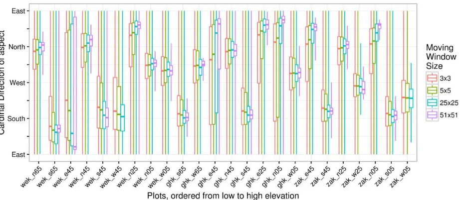
The derivation of geomorphological parameters is highly scale depended. Figure 11 shows the variability of each plots aspect according to different moving windows. It cannot be expected that each plot faces a certain cardinal direction in a perfect manner. However, one would expect that the overall aspect of the plot would satisfy the general expectation, i.e. that a plot on an eastern slope faces east. That this is not the case shows the variability of the micro-topography as depicted in Figure 11. The range of expositions is 360 degrees for almost all plots. Only when the moving window size is increased, and thus a generalization applied, the variability is reduced and the median value of the cell expositions approaches its expected value.
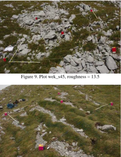
Based on the slope parameter we are able to derive a roughness parameter for each plot. We use the standard deviation of slope (SDslope) as a roughness measurement as proposed by Grohmann et al. (2011). SDslope describes sudden changes in the topography, i.e. the slope values, with high values. According to Grohmann et al. (2011) this index is well suited for terrain analysis and is able to detect fine scale relief at a variety of scales. Figure 8 shows the median roughness for each plot as the median SDslope. The figure shows a high roughness for plot wek_s45 (Figure 9) and low for plot ghk_e45 (Figure 10). It can be seen that the plot in Figure 9 includes a lot more large rocks than ghk_e45 which raises the roughness index. Ghk_e45 on the other hand includes more grass areas which cannot be modelled by our point cloud in detail and is therefore depicted as a rather smooth surface.
Figure 8. Plot roughness as the mean standard deviation of slope. Moving window size is 9x9 pixels.
Figure 9. Plot wek_s45, roughness = 13.5
Figure 11. Distributions of cell aspects for each plot by moving window sizes. Vertical lines represent the range of absolute values, horizontal lines are the median values and the box margins are the 25th and 75th quantile. Plot names are abreviations for the
summits, the cardinal directions and altitudes below the HSP.
4. DISCUSSION
The close-range and high-resolution aspect of this photogrammetrical approach requires for careful analysis of derived topographic parameters. Usually, digital elevation models have a resolution that masks the micro-topography and therefore allows for fast quantification of regions of different scales. However, our small-scale approach detects even the smallest changes in the local topography. In the larger scope of the project these microtopographic reliefs become important as possible refugia for species threatened by climate change.
Cast-shadow is problematic if the shadow is cast by the photographer. In the field and on a tight schedule one cannot choose much when to photograph a certain plot. Especially during times of low sun inclinations and if a hillside faces the sun the shadow of the photographer becomes quite long and may reach far into the plot that is being photographed. The SIFT algorithm is robust and invariant to shadows to a certain extend. However, if the same shadow pattern reappears in different locations the algorithm may become confused when correlating the images and computing the tie-points.
On the other hand, cast shadows by topographic obstacles are less problematic because they move slow enough compared to the acquisition speed of images. If however the contrast between the shadow and the surrounding terrain is very strong the shadow will be a mostly black surface on which no tie-point can be found of the noise becomes high.
Especially while capturing the oblique imagery during morning and evening hours, the position of the sun relative to the plot of interest becomes relevant. Depending on the time of the day the sun has a low inclination, which may result in lens flares when taking pictures against the sun. These lens flares may not be visible on the camera display, due to very bright lightning conditions, and may result in less images suitable for the SfM workflow.
Dense and high vegetation itself proves to be problematic. While the MEDIALPS project aims at mapping vegetation location properties the vegetation itself sometimes obscures the
surface which’s parameters are to be quantified. It has to be assumed that the surface of the vegetation represents the topographic properties of the ground. Then close range photogrammetry can produce valid parameters that describe vegetation location properties.
Wind is omnipresent on mountain summits. This make the image acquisition difficult as well as shakes taller vegetation, especially grasses. The constant movement of grass and leaves make a reconstruction based on SfM impossible and results in data gaps in the dense point cloud.
The processing of many high resolution point clouds needs large data storage capabilities. A single cloud of 3 m² produces several tenth of gigabytes. This makes the parallel processing of a large number of point clouds difficult. If intermediate results need to be stored for analysis purposes external data storage solutions are needed.
Our solution to generate high-detail elevation model of micro-relief is lightweight and low-cost. In the field, nothing more than a consumer grade camera and some targets for scaling are required. In the office, a reasonably powerful personal computer is sufficient. Larger project such as the one presented in Section 2.1 need more processing power which can be provided by research institutions or via cloud computing, for example.
5. OUTLOOK
The processing as outlined in Section 2 and 3 will continue in the other regions mentioned in Section 2.1. In order to compute the dense point clouds and topographic parameters we will make further use of the high performance cluster (HPC) at the University Innsbruck.
models will be computed to further differentiate between microscale locations. Thus, we will be able to determine if a population is already in a refugial spot or if it is in danger of displacement by competition or climate factors.
Furthermore, we will explore upscaling approaches to embed the small-scale results in a regional context. Especially shadowing effects from surrounding summits and their cast shadows will play an important role.
ACKNOWLEDGEMENTS
This work has been conducted within the project MEDIALPS (disentangling anthropogenic drivers of climate change impacts on alpine plant species), which is funded by the Earth System Sciences Program of the Austrian Academy of Sciences. The project was supported by the Austrian Federal Ministry of Science, Research and Economy as part of the UniInfrastrukturprogramm of the Focal Point Scientific Computing at the University of Innsbruck.
Images for the structure-from-motion approach used in the examples above were captured by GLORIA during the 2015 summer field campaign.
REFERENCES
CloudCompare Wiki, 2015. SOR Filter. http://www.cloud compare.org/doc/wiki/index.php?title=SOR_filter (4.4.2016).
Grohmann, C.H.; Smith, M.J. & Riccomini, C., 2011. Multiscale Analysis of Topographic Surface Roughness in the Midland Valley, Scotland. IEEE Transactions on Geoscience and Remote Sensing 49/4: 1200 – 1213.
Institut national de l’information géographique et forestière (IGN), 2016. MicMac, Apero, Pastis and Other Beverages in a Nutshell. Available via Mercurial repository https://culture3d:[email protected]/hg/culture3d (6.1.2016).
Pauli, H., Gottfried, M.; Dullinger, S.; Abdaladze, O.; Akhalkatsi, M.; Alonso, J.L.B.; Coldea, G.; Dick, J.; Erschbamer, B.; Calzado, R.F.; Ghosn, D.; Holten, J.I.; Kanka, R.; Kazakis, G.; Kollar, J.; Larsson, P.; Moiseev, P.; Moiseev, D.; Molau, U.; Mesa, J.M.; Nagy, L.; Pelino, G.; Puscas, M.; Rossi, G.; Stanisci, A.; Syverhuset, A.O.; Theurillat, J.-P.; Tomaselli, M.; Unterluggauer, P.; Villar, L.; Vittoz, P. & Grabherr, G., 2012. Recent plant diversity changes on Europe’s mountain summits. Science 336: 353 – 355.
Pauli, H., Gottfried, M., Lamprecht, A., Niessner, S., Rumpf, S., Winkler, M., Steinbauer, K. and Grabherr, G., 2015. The GLORIA field manual – standard Multi-Summit approach, supplementary methods and extra approaches. 5th edition. GLORIA-Coordination, Austrian Academy of Sciences & University of Natural Resources and Life Sciences, Vienna.
Scherrer, D. & Körner, C., 2010. Infra-red thermometry of alpine landscapes challenges climatic warming projections. Global Change Biology 16/9: 2602–2613.
Scherrer, D. & Körner, C., 2011. Topographically controlled thermal-habitat differentiation buffers alpine plant diversity
against climate warming. Journal of Biogeography 38: 406 – 416.
Maps and digital elevation models
European Environment Agency (EEA), 2016. European digital elevation model (EU-DEM). Available at http://www.eea. europa.eu/data-and-maps/data/eu-dem.
GIS-Steiermark, 2016. Geländemodell 10 m. Available at http://www.gis.steiermark.at/.
Instituto Geográfico Nacional (IGN): MDT05/MDT05-LIDAR, 2016b. Available at http://www.ign.es.
Ufficio Sistemi Informativi - Servizio autorizzazioni e valutazioni ambientali, 2016. LIDAR rilievo 2006/2007/2008. Available at http://www.territorio.provincia.tn.it/portal/server. pt/community/lidar/847/lidar/23954
United States Geologocal Survey (USGS), 2016. Shuttle Radar Topography Mission (SRTM): Available at https://lta.cr.usgs. gov/SRTM.
MapQuest, 2016. Terrestrial imagery by NASA. Accessed via OpenLayers QGIS Plugin (version 1.3.6). https://github.com/ sourcepole/qgis-openlayers-plugin (30.3.2016).
Software
CloudCompare (version 2.6.3) [GPL software], 2015. Retrieved from http://www.cloudcompare.org/.
Darktable (version 2.0.3) [GPL software], 2016. Retrieved from https://www.darktable.org/.
GRASS GIS (version 7.0.3) [GPL software], GRASS Development Team, 2016. Retrieved from https://grass. osgeo.org/.
MicMac (1.0) [CeCILL-B software], Institut national de l’information géographique et forestière (IGN), 2016. Retrieved from Mercurial repository https://culture3d:culture3d@geo portail.forge.ign.fr/hg/culture3d.