AUTOMATIC BUILDING EXTRACTION AND ROOF RECONSTRUCTION IN 3K
IMAGERY BASED ON LINE SEGMENTS
A. K¨ohna∗, J. Tiana, F. Kurza a
German Aerospace Center (DLR), Remote Sensing Technology Institute (IMF), 82234 Weßling, Germany -(alexander.koehn, jiaojiao.tian, franz.kurz)@dlr.de
Commission III, WG III/4
KEY WORDS:Building detection, line segment detection, DSM, morphological filtering, RANSAC, plane fitting, vegetation identi-fication
ABSTRACT:
We propose an image processing workflow to extract rectangular building footprints using georeferenced stereo-imagery and a deriva-tive digital surface model (DSM) product. The approach applies a line segment detection procedure to the imagery and subsequently verifies identified line segments individually to create a footprint on the basis of the DSM. The footprint is further optimized by mor-phological filtering. Towards the realization of 3D models, we decompose the produced footprint and generate a 3D point cloud from DSM height information. By utilizing the robust RANSAC plane fitting algorithm, the roof structure can be correctly reconstructed. In an experimental part, the proposed approach has been performed on 3K aerial imagery.
1. INTRODUCTION
Automatic building extraction and reconstruction from very high resolution remote sensing images are difficult tasks. The detec-tion accuracy strongly depends on image quality and building shapes. In addition to 2D information from spectral and panchro-matic images, height information from digital surface model (DSM) has received increasingly attention for automatic building extraction.
A considerable amount of studies addresses DSM-assisted build-ing footprint extraction. Some of them fuse data from different sensors, chiefly multispectral images and LiDAR-derived DSMs (Matikainen et al., 2010; Hermosilla et al., 2011; Grigillo and Kanjir, 2012). Those studies, however, rely on different data sources which may imply difficulties concerning the availability and temporal coincidence of the data. Exploiting the potentials of a single platform could yield a solution. Hence, a number of authors directly extracted footprint shapes from LiDAR point clouds (Wang et al., 2006; Zhang et al., 2006; Arefi et al., 2008) or nadir RGB imagery (Shorter and Kasparis, 2009). Stereo images also provide possibilities for detecting building geometries using optical and height information derived from the same data source (Arefi and Reinartz, 2013; Tian et al., 2014) or solely height infor-mation (Weidner, 1997). Photogrammetric techniques have been used to extract three-dimensional line segments for 3D model generation (Zebedin et al., 2008). These line segments, however, require a good perspective coverage of the scene in order to be useful for building extraction. We therefore studied the potentials and limitations of extracting line segments from individual im-ages used for DSM generation and subsequently verifying them on the basis of the DSM.
A major constraint of directly inferring building footprints from DSM data is the presence of vegetation. Several approaches ad-dress this issue, e.g. by applying a Normalized Difference Veg-etation Index (NDVI) mask to the image (Grigillo and Kanjir, 2012), computing the variance of surface normal vectors within the DSM (Weidner, 1997) or segmenting a RGB image and then
∗Corresponding author
removing color-invariant segments indicating vegetation (Shorter and Kasparis, 2009). However, spectral identification of vegeta-tion is not reliable when an infrared channel is missing, especially when vegetation is (partially) cast over by shadows from adja-cent structures. It is further compromised when the acquisition time of the images does not coincide with the growing season. On the other hand, the variance of surface normals may not be a reliable indicator for vegetation if there is noise present in the DSM (see section 3.1). Therefore, another geometric criteria is proposed by applying a line segment detection algorithm to the aerial image and a standard deviation threshold to the underlying DSM. In contrast to man-made structures, line segments detected in canopies are expected to be less directional.
In a last step of building reconstruction, the detected building footprints are segmented to obtain simpler building geometries. A RANSAC-based plane fitting procedure is applied to the pixels in each segment by which 3D building roofs are reconstructed.
2. METHODOLOGY
The methodology is divided into four sections. We will first de-scribe the segmentation of the whole scene to obtain image sub-sets of individual buildings. Line segments are then identified and filtered to derive a raw building footprint. In an optimization step, morphological filtering is applied to improve the footprint shape. Eventually, the roof shape is extracted using RANSAC.
2.1 Selection of building candidates
In a first step, the DSM was normalized based on morphological grayscale reconstruction (Vincent, 1993). White morphological reconstruction can extract off-terrain objects and removes small-scale variations from a dark background. We will subsequently call this product normalized DSM (or nDSM).
corresponds to about 4000 pixels at 9 cm resolution), the remain-ing regions were considered as buildremain-ing candidates. Every build-ing candidate was then subsetted from both nDSM and RGB im-age with a rectangular buffer of 200 pixels around its outermost pixels.
2.2 LSD algorithm and line segment selection
The Line Degment Detector (LSD) proposed by von Gioi et al. (2012) identifies line segments by region growing of pixels that display the same brightness gradient and orientation in panchro-matic images. Several mechanisms prevent the algorithm from detecting noisy features or growing too large line segments which is not present in the well-established Hough transform line detec-tion algorithm (von Gioi et al., 2010).
Hence, we first transformed the RGB aerial image to a panchro-matic version. A first run of the LSD algorithm was used to identify the most dominant orientation of line segments present in the image (Fig. 1). There are two ways to proceed. The most intuitive one is to rotate every line segment according to the dominant orientation to align the bulk part of segments with the coordinate axes. However, if high-level languages like Python are used which utilizes the computational advantage of low-level languages, namely C, in its libraries, it may also be conceivable to rotate the whole image instead and repeat the line segment detection. We therefore chose the second approach. For a bet-ter understanding of the proposed approach, Figure 2 describes the footprint detection workflow by using an exemplary building. The rotated image and nDSM subsets are shown in Figure 2a and 2b. We accepted that another run of the LSD algorithm on the rotated dataset (Fig. 2c) is likely to produce slightly different results. We made the assumption that most buildings are rectan-gular which greatly boosts the introduced algorithm and is true for a large fraction of buildings in the study area. By also com-puting the chi-squared test for homogeneity (p-value set to 0.05), any building candidate featuring an equal distribution of line seg-ment orientations was discarded as this strongly indicates either vegetation or non-rectangular building footprints (e.g. circular or elliptical shapes).
To account for the image artifacts initially mentioned, all remain-ing line segments were checked for their position in the nDSM. If they fell below the set height threshold of 2 m, they were re-moved. The rest was classified by the height gradients to both
Figure 1: Distribution of line segment angles in a rectangular building (where 0◦corresponds to an horizontal orientation)
Figure 2: Footprint detection workflow; (a) rotated panchromatic aerial image, (b) normalized DSM (nDSM), (c) detected line seg-ments using the LSD algorithm, (d) line segseg-ments fulfilling the gradient criteria, (e) extended line segments that fulfill the orien-tation criteria, (f) averaged grids, (g) thresholded image filtered by standard deviation, (h) image after morphological filtering
Figure 3: Principle of gradient classification. In the upper cross-section, black/red dots represent line segments while the lines to both sites are their respective gradients. Different gradient com-bination options are displayed below.
the RGB image. In accordance with the assumption of rectan-gular buildings, the algorithm eventually selected only those line segments that were aligned with or perpendicularly orientated to the major orientation within a threshold interval of±5◦.
2.3 Footprint generation and optimization
The remaining line segments were then rotated to the nearest co-ordinate axis and extended over the whole image. Since we only took rectangular lines, one of those axes usually lies within 5◦of
each line segment. The result is a grid structure segmenting the building in multiple parts (Fig. 2e). This approach is used by a number of authors, including Zebedin et al. (2008) and Grigillo and Kanjir (2012). Non-rectangular grids are equally conceivable and were used by Zebedin et al. (2008). The statistical mean was then derived from the underlying nDSM for every grid (Fig. 2f). We obtain a measure for homogeneity of each grid by means of standard deviation (σof 3.5) which is useful to filter out vegeta-tion close to buildings, interpolated areas and grids which do not correspond to actual geometries in the scene. By only keeping the largest footprint within the current extent, intersecting extents are less likely to mutually update footprints other than the currently processed one (Fig. 2g).
In order to filter out small-scale variations in the footprint bound-ary, every candidate underwent morphological erosion with sub-sequent dilation (Fig. 2h). Considerations on the size of the structuring element are required. If a part of a building or the building as a whole is removed by erosion, it cannot be restored to its initial extent using dilation. If the structuring element is too small, it will not succeed in removing erroneous variations in the boundary region. The choice of an optimal size, therefore, de-pends on the prevailing type of land-use; industrial zones might require a larger structuring element than residential areas as the general building extent is larger. We chose a 100×100 pixel square which unlike a disk-shaped structuring element does not round off corners.
The individual building footprints are eventually rotated and re-assembled to their initial position in the image.
2.4 Roof structure reconstruction
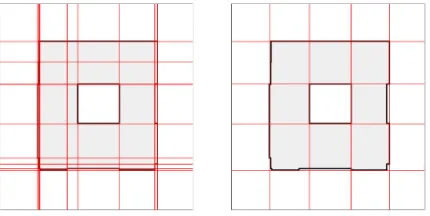
Roof structure reconstruction is a crucial step towards automatic extraction of 3D models from DSM data. Having produced a building footprint in the previous steps, we can generate a 3D point cloud by masking the initial nDSM. As complex building roofs often consist of multiple planar surfaces, we first segmented the image into simpler rectangular features based on the general outline of the building. Kada and McKinley (2009) used the term cell decomposition for a similar approach by referring to Foley et al. (1990). The segmentation of the building into cells is use-ful as it prevents plane fitting through noncontiguous parts of the building. Segmenting the image based on every variation of the outline is, however, impractical as it creates a large number of very small segments (Fig. 4, left). Instead, we kept only those lines that feature the longest building edge within a lateral buffer of 15 pixels to each side (Fig. 4, right). It is conceivable at this point to apply a further generalization step to the footprint fol-lowing the cell outline which would make the computation of a generalized building block model with roof (LOD2; Arefi et al. 2008) less complex. This is, however, not implemented here.
Figure 4: Cell decomposition without (left) and with removal of lines extrapolated from short footprint edges (right)
Random Sample Concensus (RANSAC) was originally conceived for line fitting but can be easily extended to plane fitting prob-lems. We implemented the RANSAC algorithm as described in Yang and F¨orstner (2010). The basic idea of RANSAC plane fitting is to randomly select three different data points from the point cloud which describe a plane in three-dimensional space. By computing the absolute distance of every other point in the point cloud to this hypothetical plane, we can divide the points into inliers and outliers by applying a distance threshold. This step is repeated for given number of iterations (e.g. 500–1000) to derive a plane hypothesis that comprises a maximum number of inliers. We then deleted those inliers from the point cloud and repeated RANSAC until the number of points is reduced to 10% of the initial size.
3. EXPERIMENTS AND DISCUSSION
3.1 3K data and preprocessing
In this study, we use an aerial imagery dataset from Karlsruhe, Germany which was acquired with the DLR 3K sensor system. The system consists of three commercially available DSLR cam-eras (one pointing at nadir, two in oblique lateral direction) en-abling a FOV of 110◦in across-track direction and 31◦in flight
km city area of Karlsruhe. The overlap in flight direction is 80%, whereas a side overlap exists only in regions, when flight strips are parallel or crossing. Thus, occluded regions appear quite of-ten in across flight direction, e.g. behind buildings, as these re-gions are not covered by the image dataset.
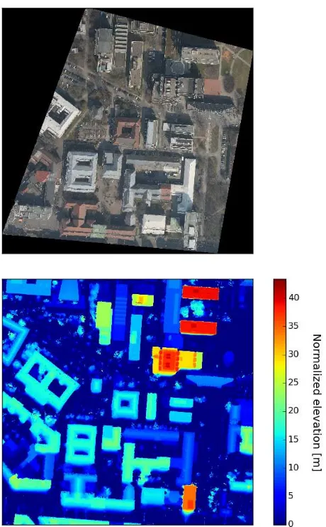
Figure 5: Input data: RGB image (above) and nDSM (below)
A high resolution DSM was derived based on the semi-global matching algorithm and taking into account multiple views with occluded regions being interpolated (d’Angelo and Reinartz, 2011). Based on the GSD of 9 cm from the imagery, a DSM resampled to 9 cm resolution was processed for all covered regions in the city of Karlsruhe. The exterior and interior orientations of all images were estimated by a bundle adjustment using the GNSS/IMU measurements. For this process, no ground based pass informa-tion was required. After outlier detecinforma-tion and smoothing of the DSM, all images were orthorectified using the derived DSM. In this study, a simple orthorectification process without ray-tracing was applied, which resulted in building edges appearing twice in occluded regions. Wherever possible, a neighboring image was used to fill the gap. Additionally, the inclined pseudo-surfaces in occluded regions lead to confusion with real inclined surfaces such as gable roofs or vegetation. It becomes difficult to avoid interpolation in densily built-up environments due to mutual oc-clusion.
3.2 Test sites
The original RGB image – comprising a size of 4469×4371 pix-els – and DSM are shown in Figure 5 and cover parts of the
south-Figure 6: Detection results using our approach
Figure 7: Detection results after thresholding the nDSM and ap-plying a morphological filter
Reference Data
Building No building
Thresholding Building 30.02% 10.81% No building 0.67% 58.51%
Overall accuracy (TP + TN) 88.53%
Our approach Building 28.53% 6.76% No building 2.16% 62.55%
Overall accuracy (TP + TN) 91.08%
Table 1: Confusion matrices of the results in Fig. 7 and Fig. 6
ern campus of the Karlsruhe Institute of Technology (KIT). The large variety of building sizes and shapes present in the subset is helpful to assess the performance of the algorithm in different urban settings.
3.3 Results and evaluation
Figure 8: Completeness and correctness of both methods for in-dividual buildings
nDSM and performing the optimization step (Fig. 7). A pixel-based statistical evaluation is recorded in Table 1.
Overall accuracy as shown in Table 1 may not be representative for the quality of the approach due to the relatively high fraction of areas without buildings. Therefore, we computed the com-pleteness and correctness of the scene as elaborated in Rotten-steiner et al. (2005):
Completeness = T P
(T P+F N) (1)
Correctness = T P
(T P+F P) (2)
where T P:= number of true positives
F N:= number of false negatives
F P:= number of false positives
If applied to the thresholded result, we obtain a completeness and correctness value of 97.83% and 73.53%, respectively. Our ap-proach yields 92.97 % for completeness and 80.84% for correct-ness. Nonetheless, Rottensteiner et al. (2005) also postulates the need for individual building assessment. From the subsequent analysis, we excluded regions that were either cut off by the im-age extent or part of a larger building complex. The latter one is due to the difficult assessment of footprints that were falsely merged or split. The results are shown in Figure 8.
The direct comparison shows the improvement of our approach over the thresholded result. The number of pixels that are false positives considerably decreased (Fig. 6–7, Tab. 1). This is espe-cially the case where vegetation is present. Some exceptions are found where trees of uniform height are closely spaced to build-ings. Given the relatively low fraction of vegetation falsely classi-fied as building, separately masking out vegetation by computing the variance of surface normal vectors (Weidner, 1997) did not improve the result but removed many inclined surfaces due the discussed interpolation. Other than that, the algorithm performs reasonably well in environments where buildings are sufficiently spaced to be distinguishable by the preselection process. How-ever, the interpolated areas are still apparent in the resulting im-age as false positives in the south-facing part of many buildings in Figure 6.
Figure 9: Found plane inliers after applying RANSAC to the building (500 iterations, distance threshold of 0.4). The colours imply different planes.
An example for detected planes in a building of average complex-ity is featured in Figure 9. RANSAC succeeds in detecting the general roof shape of most simple buildings and many more com-plex shapes. The cell decomposition performed on more comcom-plex shapes sometimes does not coincide with the roof architecture leading to some detection errors in edge regions.
3.4 Discussion
meet-ing the criteria set by the algorithm. At the same time, very short edges feature less and shorter line segments implying a higher chance of being filtered out by the orientation criteria. The geo-referenced images are partly distorted where height information was too sparse. This contributes to the low line segment density at the edges in Figure 2c–e pointing North and East, respectively. It gets even more complex if the boundary is a low-contrast zone which emphasizes the limitations of the used line segment detec-tion method. Local contrast enhancement could solve some of these issues but it may be more appropriate to utilize the mul-tiperspective information that 3K imagery provides. A simple brute force approach could repeat the line detection using dif-ferent viewing angles and/or individual RGB bands and eventu-ally merge all identified line segments for further processing. An alternative was presented by Zebedin et al. (2008) who instead photogrammetrically derived line segment from mutliple views on the same scene. However, 3K data may not have enough view angles for this approach.
Larger building complexes or roofs with regular linear patterns - predominantly saw-tooth and corrogated iron roofs as well as roof-mounted solar arrays - typically result in a very large num-ber of line segments of parallel orientation to the building bound-ary. In this instance, extended line segments project onto other parts of the building and create polygons that would otherwise not emerge or create small-scale variations in the footprint boundary since this part of the DSM is often fuzzy. This issue is addressed by testing the homogeneity of the grid and by the optimization step.
There is also the issue of the large number of assumptions that en-ter our model in the form of thresholds. Even though it performed reasonably well on the used dataset, it may be necessary to adjust these parameters depending on the sensor and scene type. This, of course, is far from ideal and we might need to apply machine learning-based techniques in future studies to ensure generaliz-ability of the model.
In comparison to simply thresholding the nDSM by a 2 m thresh-old and applying the same optimization procedure to the full im-age, the building boundaries in the present approach are more distinct and linear but vegetation is still present in both results. This would cause unwanted geometries when roof detection is applied to the respective areas. Furthermore, the structuring ele-ment partly creates a staircase effect if the building boundary is not aligned to the images axes. This is especially emphasized in the thresholded result. Nonetheless, we will need to apply more sophisticated approaches by other authors on 3K data in order to obtain more helpful conclusions about the quality of our ap-proach.
4. CONCLUSION
We showed that building footprint detection using line segments and a noisy nDSM produce results that can be used for 3D model generation. First, we segmented the image in small processing units and applied the Line Segment Detection algorithm. By suc-cessively filtering the resulting line segments, we obtained candi-date lines of the building outline. We utilized these lines on the nDSM to create a raw building footprint which was further opti-mized using morphological filtering. Some false alarms remain if small buildings and densely built-up areas are present which is mainly due to limitations of optical line segment detection and the image quality. Nonetheless, we think it is possible to over-come these problems by testing alternate line detection methods. In future work, we also need to allow non-rectangular footprints and dynamic thresholds.
As for the plane detection, visual evaluation of the obtained planes show a good agreement with the expected roof shape. Logical subsequent steps would include a comparison of faces of neigh-boring building cells whether they have a similar spatial orien-tation and to merge them where appropriate. We also need to address the accuracy assessment of the RANSAC results by us-ing ground truth information. Future research may target fully automatic 3D model generation based upon the detected building footprint and roof architecture.
ACKNOWLEDGEMENTS
The authors would like to thank Tom Kneiphof (University of Bonn) for his helpful remarks on the RANSAC algorithm.
REFERENCES
Arefi, H. and Reinartz, P., 2013. Building reconstruction us-ing dsm and orthorectified images. Remote Sensing 5(4), pp. 1681–1703.
Arefi, H., Engels, J., Hahn, M. and Mayer, H., 2008. Levels of detail in 3d building reconstruction from lidar data. In: IS-PRS Remote Sensing and Spatial Information Sciences, Vol. 37, Part B3b, pp. 485–490.
d’Angelo, P. and Reinartz, P., 2011. Semiglobal matching results on the isprs stereo matching benchmark. In: ISPRS Hannover Workshop 2011: High-Resolution Earth Imaging for Geospa-tial Information, Vol. 38(4), pp. 79–84.
Foley, J. D., van Dam, A., Feiner, S. K. and Hughes, J. F., 1990. Computer Graphics: Principles and Practice. 2 edn, Addison-Wesley.
Grigillo, D. and Kanjir, U., 2012. Urban object extraction from digital surface model and digital aerial images. ISPRS Annals of the Photogrammetry, Remote Sensing and Spatial Informa-tion Sciences 1(3), pp. 215–220.
Hermosilla, T., Ruiz, L. A., Recio, J. A. and Estornell, J., 2011. Evaluation of automatic building detection approaches com-bining high resolution images and lidar data. Remote Sensing 3(6), pp. 1188–1210.
Kada, M. and McKinley, L., 2009. 3d building reconstruc-tion from lidar based on a cell decomposireconstruc-tion approach. In: U. Stilla, F. Rottensteiner and N. Paparoditis (eds), CMRT09. IAPRS, Vol. XXXVIII, Part 3/W4, pp. 47–52.
Kurz, F., T¨urmer, S., Meynberg, O., Rosenbaum, D., Runge, H., Reinartz, P. and Leitloff, J., 2012. Low-cost optical camera systems for real-time mapping applications. Photogrammetrie-Fernerkundung-Geoinformation 2012(2), pp. 159–176.
Matikainen, L., Hyypp¨a, J., Ahokas, E., Markelin, L. and Kaarti-nen, H., 2010. Automatic detection of buildings and changes in buildings for updating of maps. Remote Sensing 2(5), pp. 1217–1248.
Rottensteiner, F., Trinder, J., Clode, S. and Kubik, K., 2005. Us-ing the dempster–shafer method for the fusion of lidar data and multi-spectral images for building detection. Information Fu-sion 6(4), pp. 283–300.
Tian, J., Cui, S. and Reinartz, P., 2014. Building change detection based on satellite stereo imagery and digital surface models. IEEE Transactions on Geoscience and Remote Sensing 52(1), pp. 406–417.
Vincent, L., 1993. Morphological grayscale reconstruction in image analysis: applications and efficient algorithms. IEEE Transactions on Image Processing 2(2), pp. 176–201.
von Gioi, R. G., Jakubowicz, J., Morel, J.-M. and Randall, G., 2010. Lsd: A fast line segment detector with a false detection control. IEEE Transactions on Pattern Analysis & Machine Intelligence 32(4), pp. 722–732.
von Gioi, R. G., Jakubowicz, J., Morel, J.-M. and Randall, G., 2012. Lsd: a line segment detector. Image Processing On Line 2, pp. 35–55.
Wang, O., Lodha, S. K. and Helmbold, D. P., 2006. A bayesian approach to building footprint extraction from aerial lidar data. In: 3D Data Processing, Visualization, and Transmission, Third International Symposium on, IEEE, pp. 192–199.
Weidner, U., 1997. Digital surface models for building extraction. In: Automatic Extraction of Man-Made Objects from Aerial and Space Images (II), Springer, pp. 193–202.
Yang, M. Y. and F¨orstner, W., 2010. Plane detection in point cloud data. In: Proceedings of the 2nd international conference on machine control guidance, Bonn, pp. 95–104.
Zebedin, L., Bauer, J., Karner, K. and Bischof, H., 2008. Fu-sion of feature-and area-based information for urban buildings modeling from aerial imagery. In: Computer Vision–ECCV 2008, Springer, pp. 873–886.