UNCERTAINTIES OF COMPLETENESS MEASURES IN OPENSTREETMAP
–
A CASE STUDY FOR BUILDINGS IN A MEDIUM-SIZED GERMAN CITYT. Törnros a, , H. Dorn a, S. Hahmann a, A. Zipf a
a Chair of GIScience, Institute of Geography, Heidelberg University, Berliner Straße 48, D69120 Heidelberg, Germany (tobias.toernros, helen.dorn, stefan.hahmann, alexander.zipf)@geog.uni-heidelberg.de
Commission II, WG II/4
KEY WORDS: VGI, map comparison, quality, uncertainty analyses
ABSTRACT:
The completeness of buildings in OpenStreetMap (OSM) is estimated for a medium-sized German city and its surroundings by comparing the OSM data with data from an official building cadastre. As completeness measures we apply two unit-based methods that are frequently applied in similar studies. It is found that the estimation of OSM building completeness strongly differ between the methods. A count ratio (number of OSM buildings / number of reference buildings) tends to underestimate the actual building completeness and an area ratio (total OSM building area / total reference building area) instead tends to overestimate the completeness within the study area. It is argued that a simple pre-processing of the building footprint polygons leads to a more accurate completeness estimation when applying the count ratio. It is also suggested to more carefully examine the areas that have been mapped in OSM but not in the reference data set (false positives). In the present study region, these values are mainly due to simplified OSM polygons and they contribute to an overestimation of the OSM building completeness when applying the area ratio.
1. INTRODUCTION
OpenStreetMap (OSM) is a growing source for spatial data. The OSM project started in 2004 and since then volunteers have contributed by mapping features like buildings, roads and land use. The OSM data are free to use and the project has become a competitor to public and commercial data providers (Neis et al., 2012). However, only a few rules restrict the uploading of data to the OSM and data completeness and data accuracy vary strongly (Werder et al., 2010). It has therefore been recommended to address the OSM quality prior to use (Al-Bakri & Fairbairn, 2012). Most of the OSM related completeness studies have focused on roads. For example, Haklay (2010) conducted a systematic study on OSM data quality by comparing the road network data with official data. Other authors have focused on building features. Fan et al. (2014) addressed the OSM building completeness in Munich, Germany. The authors concluded that the buildings in Munich are mapped almost completely in terms of covered area. Building attributes (including e.g., building height) were, however, less frequently available within the city. Kunze et al. (2013) and Hecht et al. (2013) derived the completeness of OSM buildings for two German federal states and found a completeness of 25% and 15% for North Rhine-Westphalia and Saxony, respectively. Furthermore, in the latter study the authors applied three different methods in order to estimate the completeness of buildings in OSM. They conclude that the choice of method can have a high effect on the estimated completeness value (Hecht et al., 2013). Furthermore, the authors point out that one of the applied methods (a building count ratio) tends to underestimate the building completeness. Another method (a building area ratio) instead tends to overestimate the completeness. Klonner et al. (2015) also addressed the building completeness and conducted a data quality analysis of building footprints in Bregenz, Austria. The authors compare the OSM data with official cadastre data and their results show a commonly applied method for estimating building completeness
Corresponding author
underestimating the actual completeness by 25-50% for certain areas (old town) with many adjoining buildings.
The over/-underestimation of building completeness may in many cases be traced back to the way the data are collected. Official data sets often rely on a precise cadastral surveying. They may furthermore incorporate address information which makes it possible to handle adjoining buildings as individual (but still connected) buildings. The OSM mapping instead relies on visual examinations of aerial images. From such images an identification of individual buildings may not always be possible. This influences the results when comparing the number of buildings available in the data sets. Another source contributing to the over/-underestimation of building completeness is inaccurate OSM mapping. If the building area is simplified it may in many cases overestimate the actual building size.
The present study is motivated by current literature indicating that commonly used methods for addressing the building completeness in OSM tend to either underestimate or overestimate the actual building completeness. In order to assess this over-/underestimation we apply and compare two methods taken from literature. We derive the completeness of buildings in OSM for a city and its surroundings and try to quantify the over-/underestimation associated with these values. This also includes an accuracy assessment of the OSM building data set. The study region is Ludwigshafen municipality (population: ~167,000; Nexiga GmbH, 2014), located in southwestern Germany.
2. METHODS
2.1 Building completeness
OSM building footprint data are compared to official reference building footprints from the ALKIS (Amtliches
Liegenschaftskatasterinformationssystem) data set provided by the Federal State Office for Surveying and Geo Information Rhineland-Palatinate in December 2014. First the OSM data (downloaded from www.geofabrik.de in April 2015) were projected to the coordinate system ETRS 1989 UTM Zone 32N used by ALKIS. Subsequently, two unit-based methods, earlier evaluated by Hecht et al. 2013, were applied in order to assess the building completeness in OSM:
=∑ �� � � �
∑ �� � × (1)
� � � � =∑ �� � �� �
∑ �� � � × (2)
where � � � = total number of OSM buildings
� � � = total number of reference buildings
� � � � = total OSM building area in m²
� � � � = total reference building area in m² = count completeness [count ratio in %]
� � = area completeness [count ratio in %]
Based on this definition and � are expected to take values from 0 to (above) 100 with 100 indicating a completeness of 100%. Values exceeding 100 imply that the OSM data set has more polygons or covers a larger area than the reference data.
The count completeness Ccountand the area completeness Carea were derived on a regular hexagonal grid. In comparison to squares and triangles, hexagons offer the advantage of more closely approximating the circle while providing the same complete coverage of the study area. We have chosen a side length of 300m as, from our perspective, this resulted in a good balance between necessary degree of detail and abstraction. Even if another side length could have some impact on the results, we believe that it does not impact the overall outcomes of the study. The grid was prepared by using the GIS tool Create Hexagon Grid (Whiteaker, 2015).
Once the grid had been prepared the area of each building footprint was derived in m². In the study we want to focus on residential, commercial and public buildings that are relevant for numerous applications, for example when estimating the building heat demand and population density in an area. In order to ensure comparability with the ALKIS dataset, buildings smaller than 20 m² were removed as recommended by Hecht et al. (2013). These small buildings are typically garages and sheds.
At the hexagon borders overlap issues may arise. For Ccount the number of buildings within each hexagon was derived based on the building centroids. Hence, each building was only counted once. When deriving the Carea the buildings lying in two or more hexagons were first split at the hexagon borders in order to avoid the building area being counted more than once. Thereafter spatial joins were conducted between the hexagon grid and the building data from both OSM and ALKIS. The output was the number of buildings, as well as the total building area in m² inside each hexagon polygon (Fig. 1). Based on these values, the remaining calculations for Ccount and Carea could be computed.
Following the calculations the uncertainty related to these values could be further examined.
2.2 Uncertainties related to building completeness
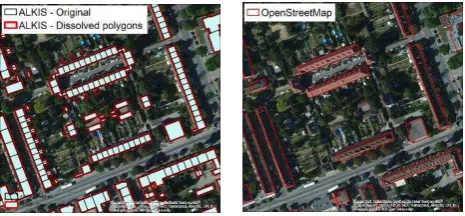
Neither the count completeness nor the area completeness pay any attention to the buildings’ geometry or their exact location inside the hexagons. Furthermore, as already mentioned, both the count completeness and area completeness may underestimate or overestimate the building completeness in certain cases (Hecht et al., 2013). Fig. 2 shows an example where using Ccount results in an underestimation of the building completeness; rows of houses are represented as individual buildings in the reference data set (Fig. 2; left). However, based on aerial images only, it is not possible in this case to distinguish individual buildings. Consequently, in OSM the rows of houses have been mapped as one long-stretched building (Fig 2; right). In cases like this the count completeness underestimates the actual building completeness.
In order to quantify the underestimation of OSM building completeness with regards to the aspect just mentioned, we apply Figure 1. Number of buildings and the total building area on a hexagon grid with a
side length of 300 meters in Ludwigshafen municipality, southwestern Germany. Background imagery (all figures): Copyright © 2010 Esri, i-cubed.
Figure 2. Original and dissolved ALKIS building polygons (reference data; left) and OSM building footprints (right).
a technique used by Klonner et al. (2015), among others. Adjoining buildings are merged into a larger building that is only counted once in Eq. 1 (Fig. 2; left). By having adjoining buildings form one building polygon the amount of reference polygons was reduced from 46,409 to 21,314 and the number of OSM buildings dropped from 14,232 to 8,140.
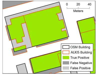
Likewise, the Careais derived from aggregated values where the spatial distribution of buildings within each hexagon polygon does not influence the estimated completeness. This method was further examined as it may cause uncertainties. The uncertainties were addressed by the concept of True Positives (TP; reference building areas that have been correctly mapped in OSM), False Negatives (FN; reference building areas not mapped in OSM) and False Positives (FP; OSM building areas not mapped in the reference data set) (Fig. 3). Also theTPrate, FPrate and FNratewere derived according to: overlapping in OSM and the reference data set. The FPrate or the commission, represents excess data present in OSM only. The FNrate or the omission, represents data absent from OSM.
In this study it is assumed that the reference buildings are complete and 100% accurate. In reality, however, that is rarely the case. In our case 98.1% of the original reference buildings are marked as having both the correct building area and location. The remaining 1.9% are marked as having non-definite coordinates and area.
3. RESULTS AND DISCUSSION
It is already known that small buildings are commonly underrepresented in OSM; seen from above they might be covered by trees or have low contrast to the ground and roads in their surroundings (Fan et al., 2014). In our study region the share of buildings smaller than 20 m² was 29.8% in ATKIS and 0.61% in OSM. For the purposes of the analysis these buildings were removed. This pre-processing step increases the estimated building completeness.
3.1 Building count: completeness and uncertainty
The building count completeness Ccount (Eq. 1) derives the percentage of the ratio: number of OSM buildings to the number of reference buildings inside each hexagon. The results show a higher overall completeness (higher Ccount) for the eastern part of the region than the western area. Especially the comparably densely built-up city centers (see Fig. 1a; central east) tend to have higher building completeness than the surrounding areas.
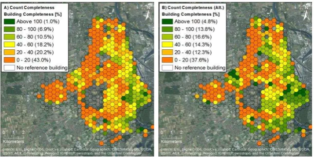
When evaluating the results in closer detail it shows 29.2% of the hexagons containing no building footprint in the reference data set. This is not surprising since the dominant land use within these areas is farmland. Further evaluation of the results reveal 43.0% of the remaining area (the hexagons polygons containing at least one reference building) having an OSM building completeness of 0-20% as derived with the count completeness (Fig. 4; left). Furthermore, the results show that 20.2%, 18.2%, 10.5% of the area have a completeness of 20-40%, 40-60% and 60-80% respectively. Further, 6.9% of the area has a completeness of 80-100%. Interestingly 1.0% of the hexagons have completeness values above 100%. A visual examination of these areas revealed that completeness above 100% mainly arose in hexagons with low building density. In these polygons, even a low number of additional OSM buildings has a high impact on Ccount. The highest values do not seem to be caused by erroneous entries in the OSM data. They rather appear to be related to the fact that OSM, when controlled with aerial images, contains correctly mapped buildings, which are not available in the reference data set. These buildings might be new and not yet exist in the reference dataset. They might also be demolished buildings, which have not been removed from the OSM dataset. The additional buildings may also be due to misinterpretations of the aerial images or incompleteness of the reference dataset, e.g., faulty locations of buildings without a proper address.
In order to investigate whether or not the count completeness tends to underestimate the actual building completeness, adjoining buildings were merged as previously described (see methods). Examining the result reveals that this pre-processing step leads to a higher estimation of the building completeness (Fig. 4; right). The amount of hexagons having a completeness between 0-60% is reduced while the amount of polygons showing a completeness above 60% increases. The mean value for completeness derived from all hexagons containing at least 10 reference buildings is increased from 33.3% to 44.9% when merging (dissolving) adjoining buildings in the pre-processing step.
With regards to the discussion above, the merging of building polygons seems to deliver a more realistic value of the building completeness. Nonetheless, it needs to be mentioned that the approach may give rise to another issue where undetailed or imprecise OSM mapping actually increases the estimation of the completeness. This issue can be observed in Fig. 2 for the reference buildings just above the middle of the figure. In the Figure 3. Building polygons from OSM (black outline) and
the reference data set ALKIS (red outline). Green areas highlights true positives (building areas overlapping in both
data sets), dark-grey indicates false negatives (reference building areas not mapped in OSM) and light-grey depict
false positives (OSM building areas not mapped in the reference data set). Here as an example from an industrial
area in Ludwigshafen.
precise reference data, the buildings form only one building when merged. The incomplete OSM buildings, however, remain as separate buildings and count as two parallel buildings. Imprecise OSM may also obstruct the correct identification of adjoining buildings and consequently cause such buildings to remain as separate polygons in the applied pre-processing step.
3.2 Building area: completeness and uncertainty
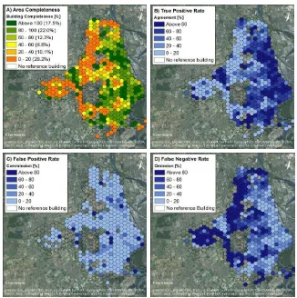
The second method for estimating the OSM building completeness is derived in percentage based on the ratio: OSM building area to reference area. In contrast to count completeness, area completeness is not negatively influenced by the issue that adjoining buildings in OSM may be mapped as one building only. This might be the main reason why using area completeness results in higher values for overall building completeness (Fig. 5a). The results show that 28.2% of the hexagons (containing at least one reference building) have a completeness of 0-20%. Furthermore, 10.1%, 8.6% and 12.3% of the polygons have a completeness of 20-40%, 40-60% and 60-80%, respectively. It also shows a completeness of 80-100% and above 100% for 22.0% and 17.5% of the hexagons, respectively. Overall, the area completeness shows a shift towards higher values in comparison to both count completeness methods presented in Fig. 4a-4b. Interestingly, a comparably high percentage of the hexagons show a completeness value above 100%. Consequently the TPrate was derived in order to quantify the proportion of correctly mapped OSM buildings. Furthermore, the potential over- or underestimation of the building completeness was assessed by computing the FPrate and FNrate. The results are shown in in Fig. 5b-5d.
The true positive rate (Fig. 5b) represents the agreement between the data sets, the quantification of the building areas overlapping in OSM, and the reference data set. Figure 5a-5b show areas with a high building completeness also having an elevated true positive rate, suggesting that a high value for building completeness (estimated with the area completeness method) relies on correctly mapped OSM building areas. Nonetheless, the TPrate shown in Fig. 5b is constantly lower than the area completeness in Fig. 5a. This fact implies that not all the buildings in OSM are mapped correctly when compared to the reference data set. With this in mind, Fig. 5b delivers additional valuable information and may actually present a more realistic estimation of the building completeness in OSM than the area completeness shown in Fig. 5a. Yet, it should also be noted that the TPrate does not account for possible offsets (in latitude and longitude) between the data sets. Furthermore, even if the OSM
buildings are digitalized well, situations occur frequently where the data sets are not agreeing completely for each building due to different level of detail and scales in the mapping. Such areas reduce the TPrate.
Examining Fig. 5c shows false positive rate overall. It also reveals a wide spectrum of rates of false positive, ranging from as low as 20% to above 80%. These high values are due to OSM building areas not included in the reference data set. By assuming the reference data set to be correct, the false positives contribute to an overestimation of the building completeness when applying the area completeness method. The false positives are consequently the reason behind the building completeness above 100% that are present in Fig. 5a. A visual analysis of those regions with a high false positive rate shows that, especially in industrial areas, complex building structures tend to be represented simplified by one larger OSM polygon (Fig. 3). In the figure it can be seen that the main reference building (having a highly irregular shape) and an outbuilding together have been mapped as a simplified rectangle in OSM. In this case, OSM overestimates the building area. The figure is also an example where the OSM user might not have accounted for the displacement due to an oblique view.
Additionally, in industrial areas outdoor spaces are often mapped as buildings in OSM; at least in our study region. However, not all false positives are caused by such mapping behavior of OSM contributors. By deriving a false positive rate the reference data set is assumed to be up-to-date and absolutely correct. In reality however, the reference dataset may also suffer from data incompleteness (cf. end of section 3.1 for possible reasons). Unfortunately this also contributes to the false positives.
The false negative rate is shown in Fig. 5d. The figure shows the percentage of reference building area that is not mapped in OSM. It reveals that areas with a high false negative rate (as expected) coincide with areas having a low building completeness.
4. CONCLUSIONS
Two methods for estimating the building completeness in OSM were applied. Comparing the results shows the tendency of a count ratio to underestimate the overall OSM building completeness. It is therefore suggested to merge adjoining buildings as a data pre-processing step before deriving this ratio. This alternative method is believed to deliver a more accurate Figure 4. Building completeness in OSM estimated with the percentage of the building
count ratio (A) and an alternative method including pre-processing of the data (B).
estimation of building completeness. The analysis also disclosed an area ratio overestimating the building completeness due to false positives (excess data present in OSM). These faulty areas may arise when detailed or complex buildings are generalized in OSM. In our study region, this undesirable mapping behavior seems to be most prevalent in industrial areas. It is furthermore suggested that the true positive rate (building areas overlapping in OSM and the reference data) offers another informative method for estimating the building completeness in OSM.
ACKNOWLEDGEMENT
The study was partly financed by the DFG Excellence Initiative. The reference geobase data have the permission notation ©GeoBasis-DE/LVermGeoRP2015-01-08. The authors would like to thank three anonymous reviewers for their useful comments and Julia Lekander for proof-reading the paper.
REFERENCES
Al-Bakri, M. and D. Fairbairn, 2012. Assessing similarity matching for possible integration of feature classifications of geospatial data from official and informal sources. International Journal of Geographical Information Science, 26(8), pp. 1437– 1456.
Fan, H., A. Zipf, Q. Fu and P. Neis, 2014. Quality assessment for building footprints data on OpenStreetMap. International Journal of Geographical Information Science, 28(4), pp. 700– 719.
Haklay, M., 2010. How good is volunteered geographical information? A comparative study of OpenStreetMap and Ordnance Survey datasets. Environment and Planning B: Planning and Design, 37(4), pp. 682–703.
Hecht, R., C. Kunze and S. Hahmann, 2013. Measuring Completeness of Building Footprints in OpenStreetMap over Space and Time. ISPRS International Journal of Geo-Information, 2(4), pp. 1066–1091.
Klonner, C., C. Barron, P. Neis, and B. Höfle, 2015. Updating digital elevation models via change detection and fusion of human and remote sensor data in urban environments. International Journal of Digital Earth, 8(2), pp. 153–171. Kunze, C., R. Hecht and S. Hahmann, 2013. On the Completeness of the OpenStreetMap Building Data. Kartographische Nachrichten, 63(2/3), pp. 73–81.
Neis, P., D. Zielstra and A. Zipf, 2012. The street network evolution of crowdsourced maps: Openstreetmap in Germany 2007–2011. Future Internet, 4, pp. 1–21.
Werder, S., B. Kieler and M. Sester, 2010. Semi-automatic interpretation of buildings and settlement areas in user-generated spatial data. In: Proceedings of the 18th SIGSPATIAL International Conference on Advances in Geographic Information Systems, San Jose, California, pp. 330–339.
Whiteaker, T.,2015. ArcGIS tool “Create Hexagon Tessellation”
available at http://tools.crwr.utexas.edu/ Hexagon/hexagon.html (25 May 2015).
Figure 5. Building completeness in OSM estimated with the building area ratio (A), as well as the true positives rate (B), false positive rate (C) and false negative rate (D).