ASSESSING MODIFIABLE AREAL UNIT PROBLEM IN THE ANALYSIS OF
DEFORESTATION DRIVERS USING REMOTE SENSING AND CENSUS DATA
J.F. Masa∗, A. P´erez Vegab, A. Andablo Reyesc, M.A. Castillo Santiagod, A. Flamenco Sandovala
a
Centro de Investigaciones en Geograf´ıa Ambiental, Universidad Nacional Aut´onoma de M´exico, 58190 Morelia, Mexico - [email protected]
b
Universidad de Guanajuato, 4500 Guanajuato, Mexico -azu [email protected] c
Centro de Investigaci´on en Alimentaci´on y Desarrollo, 83304 Hermosillo, Mexico - [email protected] b El Colegio de la Frontera Sur, San Cristobal de las Casas, Mexico - [email protected]
Commission II, WG II/4
KEY WORDS:Modifiable areal unit problem, Scale, Aggregation, Spatial analysis, Deforestation drivers
ABSTRACT:
In order to identify drivers of land use / land cover change (LUCC), the rate of change is often compared with environmental and socio-economic variables such as slope, soil suitability or population density. Socio-economic information is obtained from census data which are collected for individual households but are commonly presented in aggregate on the basis of geographical units as municipalities. However, a common problem, known as the modifiable areal unit problem (MAUP), is that the results of statistical analysis are not independent of the scale and the spatial configuration of the units used to aggregate the information. In this article, we evaluate how strong MAUP effects are for a study on the deforestation drivers in Mexico at municipality level. This was done by taking socio-economic variables from the 2010 Census of Mexico along with environmental variables and the rate of deforestation. As population census is given for each human settlement and environmental variables are obtained from high resolution spatial database, it was possible to aggregate the information using spatial units (”pseudo municipalities”) with different sizes in order to observe the effect of scale and aggregation on the values of bivariate correlations (Pearsons r) between pairs of variables. We found that MAUP produces variations in the results, and we observed some variable pairs and some configurations of the spatial units where the effect was substantial.
1. INTRODUCTION
Land use/cover change (LUCC) is significant to a large range of aspects related to global environmental change and has received increasing attention from scientists and decision makers. Over the last decades, a broad range of studies have been carried out to monitor, evaluate and project LUCC with a particular empha-sis on deforestation. Many studies of LUCC are based on remote sensing and census data using spatial analysis approaches. Mul-tidate images are classified in order to monitor LUCC and spatial variables, expected to be the drivers of changes, are integrated in a GIS database. Then, the rate of change (e.g. rate of deforesta-tion) is often compared with environmental and socio-economic variables such as slope, soil suitability or population density in order to identify and assess the effects of the drivers by means of a statistical index. Socio-economic information is obtained from census data which are collected for individual households but are commonly presented in aggregates on the basis of geographical units such as counties, municipalities or states. A common prob-lem is that the results of statistical analysis are dependent of the scale and the spatial configuration of the units used to aggregate the information. According to Openshaw (1984) , this problem, known as the modifiable areal unit problem (MAUP), has two components: the scale problem and the aggregation (or zoning) problem. The scale problem is the variation in results observed when the data are aggregated into sets of increasingly larger units of analysis. The zoning problem is related to the variations in results observed when the analysis is done using the same num-ber of alternative units. Some works indicate that the MAUP can cause variations of the correlations from -1 to +1 by judicious placement of zone boundaries (Openshaw, 1984; Openshaw and
∗Corresponding author
Rao, 1995). However, Flowerdew (2011) used a large data set from the English Census and did not found large differences be-tween correlations at different scales in the majority of the cases. In Mexico, most of census information is available at municipal level. In 2010, there were 2456 municipalities, which area ranges from a few km2to more than 53,000 km2with an average area of 796 km2. The objective of this study is to evaluate how strong MAUP effects are on the assessment of deforestation drivers in Mexico using municipality-based data.
2. MATERIALS AND METHODS
We used socio-economic variables from the 2010 Census of Mex-ico from the National Institute of Statistics and Geography IN-EGI (2010) at human settlement level along with the marginalisa-tion index calculated by the Namarginalisa-tional Commission of Populamarginalisa-tion CONAPO (2010) using information of housing, schooling and incomes from INEGI. We used also topographic indices (slope and elevation) obtained from theShuttle Radar Topography Mis-siondigital elevation model (http://www2.jpl.nasa.gov/srtm/) and the forest tree cover and forest loss data from theGlobal Forest Changedatabase (http://earthenginepartners.appspot.com/science-2013-global-forest; Hansen et al., 2013). Table 1 shows the source and the resolution of the variables used in the study. All spatial and statistical analysis were carried out using the open source program R (R Core Team, 2013; Hijmans, 2015).
Study area encompasses about 111,360 km2located in the central part of Mexico. Based on the municipal average area, expected number of municipalities for this area is 140. To test the zoning effect of MAUP we generated Thiessen polygons around 140 ran-dom points. Each Thiessen polygon was used as an analysis unit The International Archives of the Photogrammetry, Remote Sensing and Spatial Information Sciences, Volume XL-3/W3, 2015
ISPRS Geospatial Week 2015, 28 Sep – 03 Oct 2015, La Grande Motte, France
This contribution has been peer-reviewed. Editors: A.-M. Olteanu-Raimond, C. de-Runz, and R. Devillers
doi:10.5194/isprsarchives-XL-3-W3-77-2015
Variables Characteristics
Source Resolution
Forest loss Forest Change 30 m
Number of inhabitants 2010 census INEGI Settlement Illiterate population (%) 2010 census INEGI Settlement Houses with dirt floor (%) 2010 census INEGI Settlement Marginalisation index 2005 CONAPO Settlement
Elevation (m) STRM DEM 90 m
Slope (degree) STRM DEM 90 m
Table 1: Input variables characteristics
(”pseudo municipality”). We computed, for each unit, the av-erage elevation, avav-erage slope, population density, proportion of illiterate population, proportion of houses with dirt floors and the rate of deforestation, computed as the proportion of forest (tree cover>10%) which presents loss during 2000-2012. As a fol-lowing step, we calculated the bivariate correlations (Pearson’s r) between pairs of variables. In order to evaluate the zoning effect, this experiment was repeated 20 times in order to assess the vari-ations of the values of correlation depending on the configuration of the units. In order to evaluate the scale effect, the number of polygons of Thiessen varied from a 1/4th, 1/2th, twice and four times the expected number of municipalities taking into account the average municipal area in Mexico. The variation of Pearson correlation values depending on zoning and scale effects was as-sessed by means of the coefficient of variation.
3. RESULTS
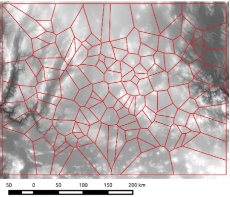
Figure 1 shows the first configuration of the 140 spatial units above the digital elevation model.
Figure 1: Limits (red) of the 140 random spatial units (”pseudo municipalities”) above the digital elevation model (grey scale)
In table 2, which shows the variation of the correlation index de-pending on the zoning effect, it can be observed that the coeffi-cient of variation ranges between 3 and 600% depending on the pair of involved variables. However, high values of the coefficient of variation correspond to weak correlation: When the coefficient of Pearson is superior to 0.5, the coefficient of variation is below 10%. It can also be observed that the minimum and maximum values of the coefficient are often different from the mean impor-tantly. These differences mean that some specific configurations of the aggregation units can conduce to very contrasting results in the statistical analysis.
Var1 Var2 Min Max Mean Stdev CoeffVar
tdef Pden 0.02 0.46 0.21 0.11 53
tdef marg -0.39 -0.00 -0.25 0.10 41
tdef dirt -0.37 0.05 -0.21 0.11 52
tdef ille -0.32 -0.05 -0.22 0.07 34
tdef slop -0.57 -0.34 -0.46 0.05 11
tdef elev -0.31 -0.09 -0.19 0.06 31
Pden marg -0.49 -0.28 -0.39 0.05 14
Pden dirt -0.27 -0.16 -0.23 0.03 14
Pden ille -0.43 -0.27 -0.36 0.05 13
Pden slop -0.23 -0.09 -0.15 0.04 28
Pden elev -0.19 -0.03 -0.13 0.04 34
marg dirt 0.80 0.92 0.87 0.03 3
marg ille 0.81 0.94 0.90 0.03 3
marg slop 0.20 0.51 0.35 0.10 28
marg elev -0.13 0.21 0.06 0.09 140
dirt ille 0.61 0.88 0.75 0.06 8
dirt slop 0.25 0.53 0.39 0.08 21
dirt elev -0.35 -0.02 -0.17 0.09 53
ille slop 0.13 0.44 0.29 0.10 33
ille elev -0.20 0.12 -0.01 0.08 598
slop elev -0.14 0.02 -0.06 0.04 74
Table 2: Minimum, maximum, mean, standard deviation and co-efficient of variation of the values of the Pearson coco-efficient of correlation with 140 units (zoning effect)
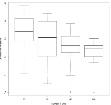
Figures 2 and 3 are box-plots which show the variation of the Pearson coefficient values between the rate of deforestation and the slope and the index of marginalisation respectively. In the case of slope, we used the absolute value of the coefficient of cor-relation to make the interpretation of the graph easier. The varia-tion of the value of correlavaria-tion is due to the change in the number of units (scale effect). As Fotheringham and Wong (1991) noticed the correlation coefficient increases when the analysis is based in larger units due to a smoothing effect by averaging, so that the variation of a variable tends to decrease as the aggregation in-creases. In the box-plot, it can also be observed outlier values of correlation which correspond to particular configuration of the units which produce extreme values of correlation. The results obtained using 35, 70, 280 and 560 spatial units are presented in the appendix.
4. DISCUSSION AND CONCLUSION
In this study, we observed the smoothing effect related with scale. For simple statistical analyses as correlation analysis and lin-ear regression, such variations can be theoretically expected and therefore are relatively well understood (Fotheringham and Wong, 1991; Jelinski and Wu, 1996). At the contrary, the zoning prob-lem is more complex and much less well understood, even for simple statistical analyses. In the present study, we observed un-predictable results related with some specific configuration of the units used to compute the indices. Figure 4 shows four different spatial configurations of the same number of aggregation units (”pseudo municipalities”) and can help understanding this be-haviour. In the two top figures (a y b), the cluster of deforestation patches belongs to one single unit, a large one for the upper left figure (a), a small one for the upper right one (b), leading to mod-erate and high rate de deforestation for the corresponding unit. In the two figures at the bottom (c y d), the cluster of deforestation is distributed among three and four aggregation units leading to even rates of deforestation.
Some studies reported that correlations varied from -1 to 1 due to the MAUP effect (Openshaw and Rao, 1995). However, these correlations were obtained using highly convoluted and there-The International Archives of the Photogrammetry, Remote Sensing and Spatial Information Sciences, Volume XL-3/W3, 2015
ISPRS Geospatial Week 2015, 28 Sep – 03 Oct 2015, La Grande Motte, France
This contribution has been peer-reviewed. Editors: A.-M. Olteanu-Raimond, C. de-Runz, and R. Devillers
doi:10.5194/isprsarchives-XL-3-W3-77-2015
Figure 2: Variation of the Pearson coefficient between the defor-estation rate and the slope due to change in the number of units
Figure 3: Variation of the Pearson coefficient between the defor-estation rate and the index of marginalisation due to change in the number of units (scale effect)
fore implausible boundaries between units. In the present study, boundaries are more simple than true boundaries due to the use of Thiessen polygons. However, as the centroid of each unit is a ran-dom point, pseudo municipalities are not realistic. For instance, some units can encompass little or, in some cases, no population at all. In future research, we will examine the effect a such unre-alistic feature on the design of units choosing randomly existing settlements with a minimum population as municipality seat (ad-ministrative center) and centroid of a spatial unit of analysis. We found that, in most of the cases, MAUP does not make large difference to the results as reported in some previous studies. However, we observed some variable pairs and some specific
Figure 4: Four configurations of aggregation units (”pseudo mu-nicipalities”) with the same number of units (zoning effect)
configurations where the effect was substantial. In future re-search, we will assess the effect of MAUP in global and local models of regression and evaluate the potential solutions reviewed by Dark and Bram (2007).
ACKNOWLEDGEMENTS
This study was supported by theConsejo Nacional de Ciencia y Tecnolog´ıa(CONACYT) and theInstituto Nacional de Estad´ıstica y Geograf´ıa(INEGI) through the projectAn´alisis espacio-temporal de la vulnerabilidad del paisaje utilizando percepci´on remota y m´etodos espaciales: un estudio interdisciplinario y multiescalar en cuatro regiones del pa´ıs.
References
CONAPO, 2010. ´Indices de Marginaci´on. Technical report, Con-sejo Nacional de Poblaci´on, M´exico D.F.
Dark, S. J. and Bram, D., 2007. The modifiable areal unit problem (MAUP) in physical geography. Progress in Physical Geogra-phy 31(5), pp. 471–479.
Flowerdew, R., 2011. How serious is the Modifiable Areal Unit Problem for analysis of English census data? Population Trends 145(145), pp. 106–118.
Fotheringham, A. S. and Wong, D. W. S., 1991. The modifi-able areal unit problem in statistical analysis. Environment and Planning A 23, pp. 1025–1044.
Hijmans, R. J., 2015. raster: Geographic data analysis and mod-eling.
INEGI, 2010. Censo de Poblaci´on y Vivienda 2010. Technical report, Aguascalientes.
Jelinski, D. E. and Wu, J., 1996. The modifiable areal unit prob-lem and implications for landscape ecology. Landscape Ecol-ogy 11(3), pp. 129–140.
The International Archives of the Photogrammetry, Remote Sensing and Spatial Information Sciences, Volume XL-3/W3, 2015 ISPRS Geospatial Week 2015, 28 Sep – 03 Oct 2015, La Grande Motte, France
This contribution has been peer-reviewed. Editors: A.-M. Olteanu-Raimond, C. de-Runz, and R. Devillers
doi:10.5194/isprsarchives-XL-3-W3-77-2015
Openshaw, S., 1984. The modifiable areal unit problem. Geo-Books, Norwich, England.
Openshaw, S. and Rao, L., 1995. Algorithms for reengineering 1991 Census geography. Environment and Planning A 27(3), pp. 425–446.
R Core Team, 2013. R: A Language and Environment for Sta-tistical Computing. R Foundation for StaSta-tistical Computing, Vienna, Austria.
APPENDIX
Var1 Var2 Min Max Mean Stdev CoeffVar
tdef Pden 0.01 0.50 0.24 0.13 53
tdef marg -0.49 -0.11 -0.34 0.10 29
tdef dirt -0.54 -0.18 -0.40 0.08 20
tdef ille -0.42 0.02 -0.26 0.11 41
tdef slop -0.61 -0.41 -0.53 0.05 10
tdef elev -0.30 0.03 -0.14 0.10 68
Pden marg -0.64 -0.37 -0.52 0.07 14
Pden dirt -0.44 -0.24 -0.34 0.06 18
Pden ille -0.62 -0.35 -0.48 0.07 14
Pden slop -0.37 0.02 -0.17 0.10 60
Pden elev -0.29 -0.03 -0.17 0.08 44
marg dirt 0.73 0.93 0.88 0.05 6
marg ille 0.89 0.97 0.94 0.02 2
marg slop -0.05 0.52 0.25 0.15 62
marg elev -0.21 0.31 0.03 0.13 424
dirt ille 0.55 0.91 0.82 0.08 10
dirt slop 0.16 0.58 0.35 0.14 39
dirt elev -0.38 0.10 -0.15 0.12 81
ille slop -0.06 0.48 0.21 0.15 73
ille elev -0.33 0.22 -0.06 0.13 197
Table 3: Minimum, maximum, mean, standard deviation and co-efficient of variation of the values of the Pearson coco-efficient of correlation with 35 units (zoning effect)
Var1 Var2 Min Max Mean Stdev CoeffVar
tdef Pden 0.00 0.59 0.23 0.14 58
tdef marg -0.44 0.06 -0.27 0.14 52
tdef dirt -0.47 0.20 -0.25 0.19 74
tdef ille -0.39 0.09 -0.22 0.13 60
tdef slop -0.58 -0.31 -0.48 0.05 11
tdef elev -0.49 -0.07 -0.22 0.11 52
Pden marg -0.57 -0.26 -0.46 0.09 20
Pden dirt -0.35 -0.15 -0.28 0.06 23
Pden ille -0.50 -0.26 -0.42 0.07 18
Pden slop -0.31 0.03 -0.14 0.08 52
Pden elev -0.26 -0.04 -0.16 0.06 39
marg dirt 0.81 0.94 0.88 0.04 5
marg ille 0.87 0.96 0.93 0.02 3
marg slop -0.04 0.50 0.28 0.15 53
marg elev -0.16 0.28 0.08 0.12 153
dirt ille 0.68 0.91 0.79 0.07 8
dirt slop 0.05 0.56 0.36 0.14 40
dirt elev -0.46 0.22 -0.13 0.15 115
ille slop -0.08 0.44 0.24 0.14 58
ille elev -0.18 0.21 0.01 0.12 1605
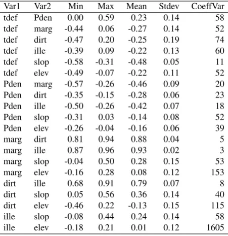
Table 4: Minimum, maximum, mean, standard deviation and co-efficient of variation of the values of the Pearson coco-efficient of correlation with 70 units (zoning effect)
Var1 Var2 Min Max Mean Stdev CoeffVar
tdef Pden 0.06 0.32 0.18 0.08 43
tdef marg -0.30 0.00 -0.23 0.07 30
tdef dirt -0.26 0.08 -0.17 0.08 46
tdef ille -0.28 -0.07 -0.20 0.05 26
tdef slop -0.48 -0.25 -0.42 0.06 15
tdef elev -0.30 -0.09 -0.19 0.04 22
Pden marg -0.39 -0.23 -0.29 0.04 13
Pden dirt -0.23 -0.12 -0.17 0.02 15
Pden ille -0.35 -0.21 -0.27 0.03 12
Pden slop -0.20 -0.07 -0.14 0.03 25
Pden elev -0.14 -0.06 -0.11 0.02 18
marg dirt 0.84 0.91 0.87 0.02 2
marg ille 0.82 0.90 0.88 0.02 2
marg slop 0.30 0.49 0.41 0.06 14
marg elev 0.03 0.18 0.11 0.04 41
dirt ille 0.68 0.80 0.74 0.03 4
dirt slop 0.34 0.53 0.43 0.06 13
dirt elev -0.17 0.00 -0.09 0.05 58
ille slop 0.25 0.41 0.33 0.05 16
ille elev -0.04 0.09 0.02 0.04 244
Table 5: Minimum, maximum, mean, standard deviation and co-efficient of variation of the values of the Pearson coco-efficient of correlation with 280 units (zoning effect)
Var1 Var2 Min Max Mean Stdev CoeffVar
tdef Pden -0.00 0.20 0.10 0.06 61
tdef marg -0.27 -0.01 -0.18 0.08 42
tdef dirt -0.20 0.10 -0.11 0.09 79
tdef ille -0.23 -0.03 -0.16 0.06 37
tdef slop -0.44 -0.08 -0.35 0.11 31
tdef elev -0.22 -0.12 -0.17 0.03 17
Pden marg -0.28 -0.16 -0.23 0.03 13
Pden dirt -0.16 -0.09 -0.12 0.02 13
Pden ille -0.26 -0.15 -0.21 0.03 13
Pden slop -0.16 -0.06 -0.10 0.03 26
Pden elev -0.13 -0.05 -0.09 0.02 22
marg dirt 0.81 0.87 0.84 0.01 2
marg ille 0.76 0.87 0.83 0.02 3
marg slop 0.33 0.50 0.41 0.04 10
marg elev 0.07 0.23 0.15 0.04 30
dirt ille 0.57 0.73 0.67 0.05 7
dirt slop 0.29 0.50 0.41 0.05 12
dirt elev -0.12 0.04 -0.05 0.04 89
ille slop 0.17 0.38 0.30 0.05 17
ille elev -0.00 0.14 0.06 0.04 63
Table 6: Minimum, maximum, mean, standard deviation and co-efficient of variation of the values of the Pearson coco-efficient of correlation with 560 units (zoning effect)
The International Archives of the Photogrammetry, Remote Sensing and Spatial Information Sciences, Volume XL-3/W3, 2015 ISPRS Geospatial Week 2015, 28 Sep – 03 Oct 2015, La Grande Motte, France
This contribution has been peer-reviewed. Editors: A.-M. Olteanu-Raimond, C. de-Runz, and R. Devillers
doi:10.5194/isprsarchives-XL-3-W3-77-2015