FILTERING OF LIDAR POINT CLOUD USING A STRIP BASED ALGORITHM IN
RESIDENTIAL MOUNTAINOUS AREAS
S. A. Hosseinia., H. Arefib and Z. Gharibb
aDep. of Civil engineering, University of Tafresh, Tafresh, Iran [email protected] bDept. of Surveying and Geomatics Engineering, University of Tehran, Tehran, Iran- ([email protected],
KEY WORDS: Segmentation, Filtering, LIDAR, Point cloud, strip based filtering
ABSTRACT:
Several algorithms have been developed to automatically detect the bare earth in LIDAR point clouds referred to as filtering. Previous experimental study on filtering algorithms determined that in flat and uncomplicated landscapes, algorithms tend to do well. Significant differences in accuracies of filtering appear in landscapes containing steep slopes and discontinuities. A solution for this problem is the segmentation of ALS point clouds. In this paper a new segmentation has been developed. The algorithm starts with first slicing a point cloud into contiguous and parallel profiles in different directions. Then the points in each profile are segmented into polylines based on distance and elevation proximity. The segmentation in each profile yields polylines. The polylines are then linked together through their common points to obtain surface segments. At the final stage, the data is partitioned into some windows in which the strips are exploited to analysis the points with regard to the height differences through them. In this case the whole data could be fully segmented into ground and non-ground measurements, sequentially via the strips which make the algorithm fast to implement.
1. INTRUDUCTION
LIDAR (LIght Detection And Ranging) is a remote sensing technique based on laser technology. It measures the two way travel time of the emitted laser pulses to determine the distance between the sensor and the ground (Wehr and Lohr, 1999). Combined with a Global Positioning System (GPS) and an Inertial Measurement Unit (IMU), LIDAR can generate a three-dimensional (3D) dense, geo-referenced point clouds for the reflective terrain surface. Compared to the traditional photogrammetric approach, LIDAR is less dependent on the weather, season, and time of the day in data collection, and can generate 3D topographic surface information more rapidly (Ackermann, 1999; Balsavias, 1999).
The collected data by LIDAR is point clouds in three dimensions. The data should be pre-processed. Pre-processing includes operations such as remove of systematic errors, filtering, feature detection and extraction, quality control and packaging [Sithole, 2005]. The original LIDAR data consist of a cloud of points returned from the terrain objects, including ground, buildings, bridges, vehicles, trees, and other non-ground features. For many applications, the non-non-ground returns must be detected, separated, and removed in order to generate the digital elevation model (DEM) (Fowler, 2001).
Different filtering methods have been proposed and accomplished. As one of the early efforts, Lindenberger (1993) introduces mathematical morphologic operators for this aim. In this method, an opening operator with horizontal structure element is first used to detect probable ground points. Points within a certain vertical distance to the estimated local average elevation are defined as ground points. An auto-regression process is then followed to correct the initial results obtained from the morphological operation. This algorithm is sensitive to the size of the structuring element. Kilian, et al. (1996) uses a series of morphologic operators with different sizes to find out the ground. To consider the local relief, Vosselman (2000)
proposes a slope-based filter that is closely related to the erosion operator using mathematical morphology. In this method, the ground is basically defined as points that are within a given slope threshold. This method may require to training for determine the parameters while implementing this filtering process (Vosselman, 2000). Additional to these algorithms, terrain slope (Axelsson, 1999; Sithole, 2001; Yoon and Shan, 2001) and local elevation difference (Wang, et al., 2001) are also used as criteria for DEM generation.
Many filtering algorithms work based on automatic extraction of ground points from point cloud (Sithole and Vosselaman, 2004; Cárdenas, 2006) that are including above mentioned methods.
Dealing to a significantly large amount of computation and memory due to the large volume of LIDAR data and their irregular sampling pattern and to facilitate the computation a Triangulated Irregular Network (TIN) is used by (Axelsson, 2000; Haugerud and Harding, 2001; Vosselman, 2000; Vosselman and Mass, 2001) to determine the filter proximity and consider the discontinuity in the terrain surface.
The fact is that DEM products can be prepared from many LIDAR service providers, but difficulties still remain in this task. The DEM generation from LIDAR data is not yet mature (Vosselman and Maas, 2001) and evaluation and manual editing is still a necessary step for DEM generation in practice (Petzold, et al., 1999; Knabenschuh and Petzold, 1999). To obtain reliable and accurate DEM products for different complexity of topography is still one important topic in institutes in the world (Crombaghs, et al., 2002; Fowler, 2001; Masaharu and Ohtsubo, 2002; Sithole, 2002). Further efforts are needed to handle complex urban areas.
resampling (sithole, 2005; Sampath and Shan 2003; Cho et al., 2004).
As one notable example, Sampath and Shan (2004) divided ground from non-ground objects with one-dimensional filtering between two consecutive points along a scan line. Sithole (2005) tested the speed of proposed segmentation algorithms, in which a point cloud was partitioned to yield a series of profiles lying at different orientations. Each profile was then segmented to produce line segments and the overlaying line segments were connected to create surfaces. Iterative processes of classification and segmentation were then conducted to classify bare earth and detailed objects.
Han et al. (2007) directly classified raw LIDAR data into homogeneous groups by an efficient method that benefits the scan-line characteristics.
In this paper we present a new approach for filtering of row LIDAR data based on strips. This paper is organized as follow: the methods are given in section 2. This section consists of 2 subsections: segmentation and strip based filtering algorithm. Segmentation sub-section is include of background in which we introduce the segmentation and assumptions that considered in segmentation procedure. Next we explain the segmentation algorithm by profile intersection. In the final, we describe the segmentation operation. In filtering we describe the filtering algorithm with total of probable cases in real world. Section 3 presents qualitative and quantitative result of scan line method. Finally, the conclusion ends the paper, presents in section 4.
2. METHODS
In this section, we describe the algorithm clearly. Base of algorithm is that first row LIDAR points segmented, then these segments using strip based filtering method divide to bare earth and objects. Performing profiling in different directions is the only common part between our algorithm and the algorithm proposed by Sithole. The operator used in our algorithm is a simple method based on distance and elevation and connected graph. The below flow is constructed segmentation-filtering framework.
Figure 1. Overall algorithm flow
2.1 Segmentation of LIDAR point cloud
The segmentation of a point cloud into smooth surfaces is the first step of the developed filter algorithm (Sithole and Vosselman, 2005). The purpose of segmentation is to obtain
higher level information from the points in a point cloud dataset (Sithole, 2005). Two points are considered to be part of the same surface if there is a smooth path between them. In this paper a novel segmentation approach is proposed. Here these two assumptions have to be considered:
Each segment encompasses only one object or a part of one object.
Points with distance and elevation proximity belong to one segment vice versa.
Here the proximity measure to be satisfied for segmentation is investigated through the exploited profiles from different directions. In the next session it will be discussed more.
2.1.1 Segmentation by profile intersection - the algorithm
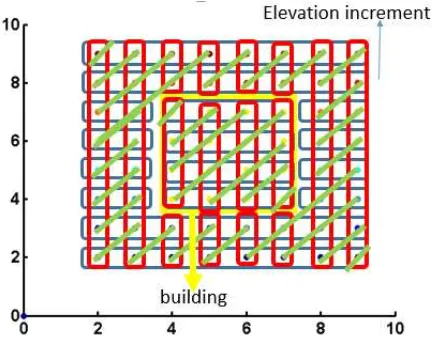
Figure 2 illustrates a simple example of the segmentation approach. In this sample the point cloud contains two surfaces; the top of a building roof -represented by the yellow square around-, and its surrounding slope bare earth. The point cloud is partitioned into three directions with the angles 0°, 90° and 30°. First along each profile, the proximity criteria are checked in order to connect probable co-linear points in the direction involved. Then the comparison of overlaid sub-profiles is done in order to find surface segments. In each profile, points are connected if they lie on the same surface when the three partitions are overlaid; points on the same surfaces interconnect. Figure 2 shows how the algorithm works for overlapping surfaces
Figure 2. Segmentation the point cloud, the building and bare earth are segmented using three different profile directions. The profile segmentation algorithm consist of three steps.
A point cloud is partitioned to yield a series of profiles lying at different orientations.
Points in the profiles are connected to yield sub-profiles. Points on the same sub-profile segment are deemed to be off the same surface.
Sub-profiles with common points in different orientations are assigned to the same segment (surface).
As the sub-profiles are made of the points with minimum height differences along, then, the third criterion can guarantee to achieve the target of segmentation here which is just to separate ground and non-ground points.
2.1.2 Partitioning the point cloud
a predefined direction in the xy plane. Because all profiles in a given direction are contiguous, points within a profile are not shared with other profiles in the same direction. In this study the value of w is set equal to one meter experimentally.
2.1.3 Segmenting the profiles
After partitioning the point cloud, each profile is in turnitself further segmented to yield sub-profiles. No two sub-profiles share common points and points in the sub-profiles are sequentially ordered. Points are allocated to sub-profiles in each profile based on distance and elevation. For each point find closest points based on elevation and distance, and then using connected graph segment wrap points that are in a segment. Points in a segment belong to a surface.
2.1.4 Surface segmentation
The overlaying of the sub-profiles yields a disconnectedgraph, G, in which the connected sub-graphs, Gi, are the desired surface segments.
When overlay profiles in different directions, points belonged to each segment inside the profiles that intersect each other, are allocated to one surface.
Because G is a disconnected graph no two segments share points in common. From the above it can be seen that the segmentation depends on:
The thickness, w, of the profiles.
The number of directions, in which the profiles are run.
Theprofile segmentation operation.
Amongst the three above, the latter one; the segmentation operation, has the greatest impact on the final segmentation results. Therefor it will be discussed in detail here.
2.2 Profile segmenting operation
To simplify the segmentation of the profiles, each profile is first transformed from a 3D frame into a 2D frame, sorted and
The principal here for profile segmentation operation is that for a point in the neighborhood of n-points the two closest to it must be on the same curve that it is on and two points are considered to be part of the same surface if there is a smooth path between them. The obtained curves are determined by distance and elevation measure. The algorithm works as follow:
In each profile, the points are sorted based on their coordinates along the profile direction
The distance and elevation differences between the points are then calculated in each profile and segment points with a group if distance and elevation difference of them be less than a predefined threshold.
Assign to each sub-profiles (segments in previous step) a unique label and later transfer labels to the sub-profiles that have common points with these sub-profiles.
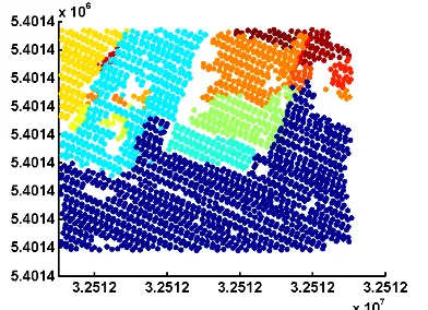
Figure 3 shows segmentation result in a small region.
Figure 3. The point cloud is profiled in different directions. After the profiles have been segmented the shape of each
sub-profile is determined.
2.3 Strip based filtering
In this section, we explain a new strategy based on strips for filtering of segments obtained in segmentation section. On this basis we begin this
2.3.1 Bare earth points detection
In order to improve the speed of algorithm, the whole dataset is partitioned into some rather smaller windows through which there is no significant and abrupt change in the trend of the earth height. The proper size for windows, therefore, should be set at least greater than the maximum size of objects inside the window. It is preferred to select the window size so that the existing outliers to be considered as ground points. Therefore at the first step of filtering analysis, in each window we sort all of points by ascending elevation and the lowest 5% are removed temporarily. Then the lowest remaining point will be labeled as the index of ground points.
Amongst the segments resulted from the previous segmentation above, the segments containing this ground point index, will be totally labeled as ground segment.
As a result of this step in the algorithm the most probable ground points are labeled and the outcome is a dataset with some labeled ground points and the other unlabeled points which are to be analysis later in the next step.
2.3.2 Strip based Filtering
Inspired from the scan line filtering method here we use a 1-D scanning mode for filtering point cloud; i.e. the whole dataset is partitioned into some narrow strips. Our algorithm is easy to implement while each strip is regarded as a single dataset. Nevertheless it will be shown that under some circumstances we may use inevitably neighboring strips for filtering to be accomplished.
In this stage, we use a moving window along the strips. Analyzing each strip as a composition of labeled and unlabeled points, we will find the strips falling into 5 different cases depending on the existence of labeled ground points in them. Case 1: higher unlabeled segment between two labeled segments. If the height difference is greater than a predefined threshold, then the unknown segment is object, else it is ground (Figure4).
Figure 4. not labebled segment between 2 labelled segments with higher elevation.
Case 2: lower unlabeled segment between 2 labeled segments. Here we may face to two different case. First is when the labeled segments belong to ground points and the second case is when they previously labeled as object points. It’s clear that in the first case the lower segment is labeled as ground points. But In the second case it is needed to check the heights with an existing ground point in the same strip. In rare cases when the current strip contains no labeled ground point, we use a ground point from the nearest neighbor strip. Then again just like the Case #1 above, labeling is done (figure 5).
Figure 5. not labelled segment between 2 labelled segments with lower elevation.
Case 3: unlabelled segment between two labelled segments without abrupt change in the heights. In this case two different conditions arise: if the two labelled segments are both co-labelled, then the third one will be of the same label and if they are of distinct labels, then the nearest segment will be used as the index (Figure 6).
Figure 6. not labelled segment between 2 labelled segments with different elevations.
Case 4: For the cases that not labelled segment is in the beginning or end of the profile, labelling done according to the next or previous labelled segment based on rules that mentioned in obove. This also holds true for the profiles that labelled segment is only in one side of not labelled segment, not necessarily in beginning or end of the the profiles.
Case 5: Briefly, the analysis of unlabeled points is done with regard to its neighboring points along the same strip. If along a strip, there is no ground point to be regarded as an index, then we must use the nearest known ground point from the adjacent strip.
If In a profile there is not a bare earth or object label we act as follow:
At the end of this stage, the whole points in dataset have a label; either ground or object points. In each scan line points with same label considered as independent group. For each group we assign a new label using average of elevations. By finding the lowest elevation label, we assign bare earth label to the point set with lowest elevation label in that scan line. Because of checking of slope condition, approximately all of bare earths in each scan line are in an almost the same elevation and very elevation differences most likely belong to non-ground objects. By assign the bare earth and object label to the points that have same segmentation label in other scan lines we continue labeling for that points with no labels based on elevation difference so that mentioned in above. These steps repeat for all of the windows that don’t share any points with previous profiles until assign a ground or non-ground label to the total of points.
The pseudo code of the algorithm is as follows:
Step 1) Assign a unique label to each group of points in segmentation section.
Step 2) Calculate average of elevations in each group.
Step 3) Fix the window with a certain size, and find out the lowest elevation in each scan line inside windows.
Step 4) Grow into ground segments for other segments in scan lines by comparison of elevations.
If segmenti –segmentj < theight : segmentj is ground, else: segmentj is non-ground.
Step 5) For next scan line, assign the ground or non-ground label to segments with same label in segmentation process. Step 6) If there are more scan lines to process, go to step 2; else, exit.
Step 7) Move the window with a certain step length, and repeat from step 3.
Here, segmenti is the average of Z-coordinate of segment i in segmentation stage, and segmentj is the average of Z-coordinate of segment j in segmentation stage. theight refers to the threshold of height difference between segmenti and segmentj.
Generally, the length of the moving window should be greater than the maximum object size yet without much change in the slope. In residential-mountain areas 45-60 m is usually suitable. The height threshold are affected by the conditions of the area and data set. theight can be changed between 1 to 3 m dependent to area condition, shape of buildings and density of non-ground objects.
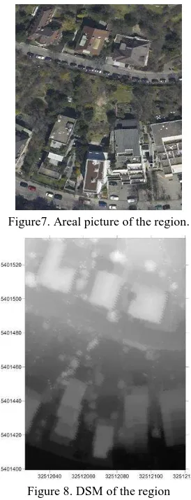
Figure7. Areal picture of the region.
Figure 8. DSM of the region
Figure 9. difference between DSM and DTM.
3. EXPERIMENTAL RESULTS
The proposed algorithm is applied to one real residential-mountain area data set. The data set comes from the city of Stuttgart in Germany and contains 22137 points with a point density of 3- 4 points /m2.
The data set contain the typical object types of modern cities, such as roads, high and low buildings, multi-story buildings, and trees. The terrain is not flat and elevation changes cover the whole area. Also roof elevation of some buildings is less than some bare earth or roads.
For segmentation a 3-m distance threshold and a 1 m height threshold are chosen for the experiment. Size of the moving
windows in filtering section is set to 45 m, and height threshold in filtering section is set to 1-m. width of strips in both segmentation and filtering section by experiment is set to 1 m. As stated before, the size of the moving window should be greater than the maximum object size. In this area which is residential-mountain we found the size 45m proper for this purpose. The value of height threshold is affected by the conditions of the area and dataset. theight can be changed between 0.5 to 1 m dependent on the area condition, shape and heights of buildings and density of non-ground objects.
The results of our proposed algorithm can be seen in the figure 7-9.
4. CONCLUSION
In this letter, we have proposed a new algorithm that uses strip-based filtering method to segment the LIDAR point cloud into the ground and non-ground points. Assigning label to the points is done with regard to the height and distance proximity in different directions. The segmentation in each profiles yields sub-profiles. These sub-profiles are then linked together through their common points to obtain surface segments. By fixing a window on the segmented data such that there is not a much elevation difference throughout the region inside the window and using a certain bar earth point allocate the bare earth label to that segment. The segment that contains this ground point, totally labeled as ground point. For profiles without common point with previous profiles, first find the lowest segment in each strip and comparison of average of elevation on each segment with the lowest elevation by considering the neighbor segments, filtering is done.
The algorithm is applied to the raw data directly, not to resampled data, to ensure that it avoids any loss of geometric accuracy. It is based on strip analysis in dataset, which makes the implementation of the algorithm more rapid and efficient. In order to improve our algorithm, we may use different directions along which the profiles are exploited to segment the whole data.
Besides, while the visual investigation of our results shows the success in separating bare earth and the objects like trees and buildings, we are to test this algorithm in the other datasets in different kinds of areas with reference DTM and DSM to check the results quantitatively.
REFERENCES
Ackermann, F., 1999. Airborne Laser Scanning—Present Status and
Future Expectations, ISPRS Journal of Photogrammetry and Remote
Sensing, Vol. 54, Issues 2–3, July, pp. 64–67.
Axelsson, P., 1999. Processing of laser scanner data—algorithms and
applications, ISPRS Journal of Photogrammetry and Remote Sensing,
Vol. 54, Issues 2–3, July, pp. 138–147.
Axelsson, P., 2000. DEM Generation from Laser Scanner Data Using Adaptive TIN Models, International Archive of Photogrammetry and
Remote Sensing, Vol. XXXIII, Part B4, pp. 110–117.
Baltsavias, E.P., 1999, Airborne laser scanning: basic relations and formulas, ISPRS Journal of Photogrammetry & Remote Sensing 54.pp.
199–214.
Cárdenas, J. L. S. And Wang, L., 2006. A multi-resolution approach for filtering LiDAR altimetry data, ISPRS J. Photogramm. Remote
Cho, W., Jwa, Y.S., Chang, H.J., and Lee, S.H., 2004. Pseudo-grid
Based Building Extraction Using Airborne Lidar Data, Int’l Archive of
Photogrammetry and Remote Sensing, XXXV, Part B3, pp. 378-381.
Crombaghs, M., S.O. Elberink, R. Brügelmann, and E. de Min, 2002. Assessing Height Precision of Laser Altimetry DEMs, International Archives of the Photogrammetry, Remote Sensing and Spatial Information Sciences, Vol. XXXIV Part 3A, Commission III,
September 9–13, Graz, Austria, pp. 85–90..
Elmqvist, M., 2002. Ground Surface Estimation from Airborne Laser Scanner Data Using Active Shape Models, International Archives of the Photogrammetry, Remote Sensing and Spatial Information Sciences,
Vol. XXXIV Part 3A, Commission III, 09–13, September, Graz,
Austria, pp. 115–118.
Fowler, R., 2001. Topographic Lidar, in Digital Elevation Model
Technologies and Applications: The DEM User’s Manual, David F.
Maune, Editor, the American Society for Photogrammetry and Remote
Sensing, Bethesda, Maryland, USA, 539 pages.Graz, Austria, pp. 165–
169.
Han, S.H.; Lee, J.H.; Yu, K.Y., 2007, an Approach for Segmentation of Airborne Laser Point Clouds Utilizing Scan-Line Characteristics. ETRI J., 29, 641-648.
Haugerud, R.A., and D.J. Harding, 2001. Some Algorithms for Virtual Deforestation (VDF) of Lidar Topographic Survey Data, Proceedings of the ISPRS workshop on Land Surface Mapping and Characterization Using Laser Altimetry, Annapolis, Maryland, The International Archives of the Photogrammetry, Remote Sensing and Spatial Information Sciences, Vol. XXXIV Part 3/W4 Commission III, pp.
203–209.
Kilian, J., Haala, N, and Englich, M, 1996. Capture and Evaluation of Airborne Laser Scanner Data, International Archive of Photogrammetry and Remote Sensing, XXXI, Part B3, pp. 383-388.
Knabenschuh, M., and B. Petzold, 1999. Data Post-processing of Laser Scan Data for Countrywide DEM Production, Proceedings of the
Photogrammetry Week, D. Fritsch and R. Spiller, Editors, pp. 233–240.
Kraus, K., and N. Pefifer, 2001. Advanced DEM Generation from Lidar Data, Proceedings of the ISPRS workshop on Land Surface Mapping and Characterization Using Laser Altimetry (Hofton, M., editor),
Annapolis, Maryland, The International Archives of the
Photogrammetry, Remote Sensing and Spatial Information Sciences, Vol. XXXIV, Part 3/W4 Commission III.
Lohmann, P., Koch, A., and Schaeffer, M, 2000. Approaches to the Filtering of Laser Scanner Data, International Archives of Photogrammetry & Remote Sensing, XXXIII, Part B3, pp. 540-547.
Masaharu, H., and K. Ohtsubo, 2002. A Filtering Method of Airborne of the Photogrammetry, Remote Sensing and Spatial Information
Petzold, B., P. Reiss, and W. Stoessel, 1999. Laser Scanning—
Surveying and Mapping Agencies are Using a New Technique for the
Derivation of Digital Terrain Models, ISPRS Journal of
Photogrammetry and Remote Sensing, Vol. 54, Issues 2–3, July, pp. 95–104.
Raber, G.T., J.R. Jensen, S.R. Schill, and K. Schuckman, 2002. Creation of Digital Terrain Models Using an Adaptive Lidar Vegetation
Point Removal Process, Photogrammetric Engineering & Remote
Sensing, Vol. 68, No. 12, pp. 1307–1316.
Sampath, A. and J. Shan., 2004. Building segmentation from raw lidar data. ASPRS annual conference, Anchorage, AK, May 5-9. CD-ROM, 5 pages.
Sciences, Vol. XXXIV Part 3B, Commission III, 09–13.
Sithole, G., 2001. Filtering of Laser Altimetry Data Using a Slope Adaptive Filter, Proceedings of the ISPRS workshop on Land Surface
Mapping and Characterization Using Laser Altimetry (Hofton, M., editor), Annapolis, Maryland, The International Archives of the Photogrammetry, Remote Sensing and Spatial Information Sciences,
Vol. XXXIV Part 3/W4 Commission III, pp. 203–210.
Sithole, G., 2005, Segmentation and Classification of Airborne Laser Scanner data. Master of Science integrated Geoinformation and Map Production, Delft University.
Sithole, G., Vosselman, G., 2005, filtering of airborne laser scanner data based on segmented point clouds, ISPRS WG III/3, III/4, V/3 Workshop "Laser scanning 2005", Enschede, the Netherlands, pp. 66-71.
Sithole,G., and Vosselman, G., 2004, Experimental comparison of filter algorithms for bare-Earth extraction from airborne laser scanning point clouds, ISPRS J. Photogramm. Remote Sens., vol. 59, no. 1/2, pp. 85–101.
Vosselman, G., 2000. Slope Based Filtering of Laser Altimetry Data, International Archives of Photogrammetry and Remote Sensing, Vol.
XXXIII, Part B3, Amsterdam 2000, pp. 935–942.
Vosselman, G., and H. Mass, 2001. Adjustment and Filtering of Raw Laser Altimetry Data, Proceedings OEEPE Workshop on Airborne Laserscanning and Interferometric SAR for Detailed Digital Elevation
Models, March 1–3, Stockholm.
Wang, Y., B. Mercer, C., Tao, J. Sharma, and S. Crawford, 2001. Automatic Generation of Bald Earth Digital Elevation Models from Digital Surface Models Created Using Airborne IFSAR, Proceedings of
the ASPRS Annual Conference, April 23–27, St. Louis, Missouri,
unpaginated CD-ROM.
Wehr, A. and Lohr, U., 1999. Airborne laser scanning—an introduction
and overview, ISPRS Journal of Photogrammetry & Remote Sensing
54.pp. 68–82.
Yoon, J.S., and J. Shan, 2002. Urban DEM Generation from Raw Airborne Lidar Data, Proceedings of the Annual ASPRS Conference,