CENTIMETER RANGE MEASUREMENT USING AMPLITUDE DATA OF TERRASAR-X
IMAGERY
P. Capaldo∗, F. Fratarcangeli, A. Nascetti, A. Mazzoni, M. Porfiri, M. Crespi DICEA - Geodesy and Geomatics Division - University of Rome ”La Sapienza”, Italy
(paola.capaldo, francesca.fratarcangeli, andrea.nascetti, augusto.mazzoni, martina.porfiri, mattia.crespi)@uniroma1.it
Commission VI, WG VI/4
KEY WORDS:SAR, amplitude, TerraSAR-X, atmospheric and geophysical corrections, land and infrastructures monitoring
ABSTRACT:
The SAR (Synthetic Aperture Radar) imagery are largely used for the environmental, structures and infrastructures monitoring. In particular, Differential SAR Interferometry (DInSAR) is a well known technique that allows producing spatially dense displacement maps with centimetre to millimetre accuracy. The SAR signal is characterized by phase and amplitude value and the DInSAR remote sensing technique allows to analyse deformation phenomena affecting both extended natural areas and localized man-made structures, by exploiting the phase difference of SAR image pairs. New SAR satellite sensors such as COSMO-SkyMed, TerraSAR-X and PAZ offer the capability to achieve positioning in a global reference frame accuracies in the meter range and even better, thanks to the higher image resolution (up to 0.20 m pixel resolution in the Staring SpotLight mode for TerraSAR-X and PAZ) and to the use of on board dual frequency GPS receivers, which allows to determine the satellite orbit with an accuracy at few centimetres level. The goal of this work is to exploit the slant-range measurements reaching centimetre accuracies using only the amplitude information of SAR images acquired by TerraSAR-X satellite sensor. The leading idea is to evaluate the positioning accuracy of well identifiable and stable natural and man-made Persistent Scatterers (PS’s) along the SAR line of sight. The preliminary results, obtained on the Berlin area (Germany), shown that it is possible achieve a slant-range positioning accuracy with a bias well below 10 cm and a standard deviation of about 3 cm; the results are encouraging for applications of high resolution SAR imagery amplitude data in land and infrastructures monitoring.
1. INTRODUCTION
New earth observation SAR (Synthetic Aperture Radar) satellite sensors, as COSMO-SkyMed, TerraSAR-X and PAZ, acquire im-agery on any point of the Earth with high resolutions, in terms of phase and amplitude value. Therefore, these data are rou-tinely and conveniently used in order to monitoring deformation phenomena impacting the Earth surface (e.g. landslides, subsi-dences, volcano deformations and glacier motions) and infras-tructures (e.g. buildings, dams, bridges). The main remote sens-ing technique to extract centimeter information from SAR data is the Differential SAR Interferometry (DInSAR), based on the phase information only (Berardino et al., 2002). Specifically, this technique is based on an appropriate combination of differential interferograms generated by image pairs characterized by a small orbital separation (baseline), in order to limit the spatial decorre-lation phenomena.
On the other hand, it is well known that DInSAR technique may suffer for lack of coherence among the considered images, and that it is particularly suited for slow deformation phenomena, due to the intrinsic need to unwrap the phase, what can be difficult in presence of displacements (much) higher than the wavelenght of the SAR signal (few centimetres). In addition, the new high resolution SAR satellite sensors offer the capability to achieve positioning accuracies in a global reference frame in the meter range and even better, thanks to the very high image resolution (up to 0.20 m pixel resolution in the Staring SpotLight mode for TerraSAR-X and PAZ) and to the use of on board dual frequency GPS receivers, which allow the determination of the SAR satel-lite orbit with an accuracy at few centimetres level.
This is the why it appeared advantageous in the last years the development of a different approach for land and infrastructures monitoring by SAR, exploiting the signal amplitude and
avoid-∗Corresponding author
ing coherence deficiency and displacement magnitudes restric-tion (Nascetti et al., 2014).
The very first idea was to evaluate the positioning accuracy of well identifiable and stable natural and man-made Persistent Scat-terers (PS’s) (e.g. corner reflectors) along the SAR line of sight. This information is of course of crucial importance in order to assess the potential of this technique to monitor the possible dis-placements of the considered PS’s. The first experiments, both using suitable corner reflectors positioned by high precision GPS surveys and natural PS’s, were carried out with stacks of TerraSAR-X SpotLight imagery, reaching a slant-range measurements ac-curacy with a bias of about 90 cm and a standard deviation of about 4 cm (Eineder et al., 2011). Then, these experiments were repeated and refined, reaching similar results as regards the stan-dard deviation but with a more and more reduced bias of about 29 cm (Cong et al., 2012) and 10 cm (this result was obtained with corner reflectors) (Balss et al., 2013) respectively.
Here we propose a partially different approach, considering only natural PS’s, where, at first, the approximate reference position of each PS is determined through a stereo approach. Then the posi-tioning accuracy of a PS along the SAR line of sight is evaluated starting from this reference position and the orbital information supplied in the SAR imagery metadata, and accounting both for signal propagation delays and for geophysical effects causing not negligible PS displacements.
the troposphere and ionosphere. Finally, it is necessary to filter out the known geophysical effects inducing periodic and secular ground displacements.
In section 2 it is outlined our methodology for the positioning ac-curacy assessment of a PS along the SAR line of sight; in section 3 the employed stereo model is recalled; in section 4 the correc-tions applied to the measured slant-ranges for atmospheric delays and geophysical effects are shortly summarized; in section 5 they are presented and discussed the main results of the investigation, carried out on a stack of 20 TerraSAR-X SpotLight images ac-quired on Berlin urban area (Germany) between February 2008 and March 2009; finally, some conclusions are drawn.
2. METHODOLOGY
The methodology proposed in this work is devoted to evaluate the positioning accuracy of a PS along the SAR line of sight using the amplitude information only.
2.1 PS absolute position estimation
Starting from an interferometric repeat-pass stack (composed by N SAR images) and using one single same side image acquired on a different orbit, it is possible to retrieve the 3D position of a PS in a global reference frame (ECEF - Earth Centered Earth Fixed) using a stereo approach. To this aim, it is at first neces-sary to measure the image coordinate of the PS both in all the stack images and in the single image and subsequently, solving the radargrammetric equations (see section 3), the PS position for each pair (one stack image with single image) can be computed. In this way, a good redundancy is introduced, computing N PS positions using N different pairs; their median is taken as robust estimation of the PS reference position.
2.2 Image coordinates measurement
An automatic matching procedure has been implemented to mea-sure the PS image coordinates in all the stack images. A patch is defined in the first stack image centered on the selected PS and a template matching is performed between this patch and a cor-responding area in all other stack images. A two steps approach was used in order to achieve a sub-pixel accuracy. First we used a moving window of 151 pixels x 151 pixels and a searching win-dow of 351 pixels x 351 pixels and we computed the Normalized Cross-Correlation (NCC) on image intensity after oversampling by a factor of two both in range and azimuth directions. Sec-ondly, after the determination of the position of the maximum NCC value, in order to refine the PS image position, we took the two corresponding patches in the master and in the slave images and we oversampled them by a factor of 100 and 10 in the range and azimuth directions respectively. Using this procedure it is possible to achieve a raster precision of 1/200 samples in range corresponding to 2.5 mm and a 1/20 samples in azimuth corre-sponding to 20 mm.
2.3 Range measurement comparison
Starting from the ECEF positions of PS and SAR sensor when imaging the PS itself (it can be computed by orbital information supplied into the metadata), it is possible to easily compute the the SAR sensor-to-PS distance and to compare it with the slant-range distance measured by the SAR sensor. The corresponding differences∆:
∆R=Slant−Rangemeasured−Distancecomputed (1)
As briefly reported in the section 4.2 the range measures are af-fected both for atmospheric and geophysical effects, which must be considered. In particular the∆Rvalues have been corrected accordingly with this equation:
∆R−T D+ID+EM=δ+ǫ (2)
where:
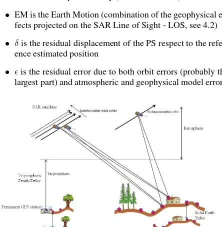
• TD is the Tropospheric Delay (see section 4.1.1)
• ID is the Ionospheric Delay (see section 4.1.2)
• EM is the Earth Motion (combination of the geophysical
ef-fects projected on the SAR Line of Sight - LOS, see 4.2)
• δis the residual displacement of the PS respect to the
refer-ence estimated position
• ǫis the residual error due to both orbit errors (probably the
largest part) and atmospheric and geophysical model errors
Figure 1: SAR acquisition geometry and slant-range corrections
It is important to underline that the residual errorǫis likely to be spatially correlated over the entire area, otherwise the point dis-placement is strictly dependent to the point location. Considering these differences, one o more stable points could be conveniently used to eliminate by differences the modelǫerror highlighting the point displacements of the points affected by displacement.
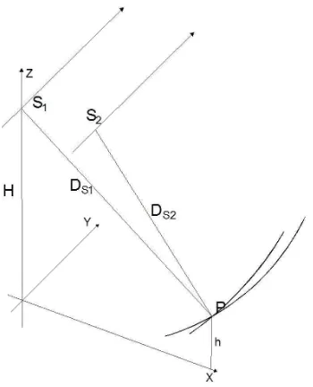
3. SAR STEREO MODEL
based on two standard equations (3): the former represents zero Doppler projection and the latter the slant range constrains (Ca-paldo et al., 2014).
Figure 2: SAR acquisition system in zero Doppler geometry
Therefore, the couple of equations in an ECEF (Earth Centered Earth Fixed) system (for example the WGS84) reads:
• XP,YP,ZPare the coordinates of the generic ground point
P in the ECEF coordinate system
• XS,YS,ZSare the coordinates of the satellite in the ECEF
coordinate system
• uXS,uYS,uZSare the Cartesian components of the satellite
velocity in the ECEF coordinate system
• Dsis the so-called “near range”
• ∆ris the slant range resolution or column spacing
• Iis the column position of point P on the image
Since the satellite angular velocity can be considered constant along the short orbital arc related to the image acquisition, the epoch of line acquisitiontcan be related to the corresponding line numberJthrough the following linear function:
t=start time+ 1/P RF·J (4)
wherestart timeis the time of start of acquisition,P RF is the Pulse Repetition Frequency. The orbit computation consists of estimation of satellite position at the epochtof each line acqui-sition according to zero Doppler geometry. In the metadata file of each SAR imagery the ECEF position and velocity of satellite related to the time are supplied through state vectors at regular in-tervals, whose numberNdepends on the considered SAR sensor.
The orbit interpolation has been performed by Lagrange polyno-mials (5), whose degree depends on the state vectors numberN.
pn(x) =y0·L0(x) +y1·L1(x) +...+yN·LN(x) =
Lagrange polynomial interpolation is enough accurate to model the short orbital segment and its well-known oscillation problems at the edges do not affect the modeling since the images are ac-quired just in the central part with respect to the supplied orbital segment. Additionally, using a standard divide and conquer algo-rithm it is possible to find in a fast and accurate way the seeked epochtwhen satellite orbit is perpendicular to the line of sight between the sensor and the generic ground point (Capaldo et al., 2014).
4. RANGE CORRECTIONS
As mentioned, in order to evaluate the positioning accuracy of a PS along the SAR line of sight it is necessary to correct for the signal propagation delays through the troposphere and iono-sphere and for known geophysical effects inducing periodic and secular ground displacements (Fig.1).
The tropospheric delay (TD), which is by far the most important correction to be applied, is close to 2.5 meters in zenith direc-tion at sea level at mid latitude, and the needed correcdirec-tion along the slant path at better than centimetre level can be estimated by GNSS phase observations collected in the area imaged by SAR, using a proper mapping function (Bonafoni et al., 2013). The ionospheric delay (ID) in X-band is in the order of few centime-tres and can be computed by a global model (e.g. Klobuchar) (Klobuchar and John, 1987). The geophysical effects consist pri-marily in the solid Earth tides (SET), polar tides (PT), crustal deformations due to ocean loading (significant close to shore-lines) (TOL), which globally can be at the level of half meter and can be corrected using the International Earth Rotation Ser-vice Conventions (McCarthy and Petit, 2003), (Petit and Luzum, 2010); moreover, geodynamics (G), crustal deformations due to atmospheric loading (variation of atmospheric pressure) (AL), glacial isostatic adjustment (significant mainly in north Europe and Canada) (GIA) and the effect of the seasonal hydrological loading (HL) have to be accounted for. All the geophysical ef-fects are grouped within the Earth motion (EM) effect.
For each PS, both the atmospheric and the geophysical effects are computed in the geodetic local system (East, North and Up) cen-tred in the PS itself, then they are summed up and projected on the SAR line of sight (LOS).
4.1 Atmospheric effects
TheZT DGP Srelative to the time of the SAR image acquisition was obtained through a linear interpolation between two consec-utive hourly values. The height correction was computed apply-ing the the NATO Standardisation Agreement - STANAG 4294 (NATO, 1997) tropospheric model. Both for the GNSS station and for the (mean) height of the imaged area theZT Dwere com-puted according to STANAG model, and their difference
∆ZT DhSAR−hGN SS was applied to getZT DSARfrom the
ZT DGN SS:
ZT DSAR=ZT DGN SS+ ∆ZT DhSAR−hGN SS; (6)
The TD is then derived from ZTD by a mapping function; if the image incidence angleθis lower than 60 degrees, a suitable map-ping function is just the simple inverse cosine (cosθ1 ). Therefore, in this case the relationship between the ZTD and the SAR image TD reads:
T DSAR=ZT DSAR
cosθ ; (7)
4.1.2 Ionospheric delay The ionospheric delay has a very small influence, within few centimeters, in the X-band (e.g. 9.65 GHz, for TerraSAR-X) and it was just computed using the Klobuchar model and the related coefficient supplied in the GPS broadcast navigation message on a two-hours basis (Klobuchar and John, 1987).
4.2 Geophysical effects
The SET, TOL and PT models are well-described in the Inter-national Earth Rotation Services (IERS) Conventions 2010 (Petit and Luzum, 2010).
4.2.1 Solid Earth Tide For the SET, which can amount up to half a meter, the free online softwaresolid.exe, developed by D. G. Milbert (National Geodetic Survey-NOAA) (http://home.com-cast.net/ dmilbert/softs/solid.htm), was used. It runs in a DOS window asking for the date (year, month number and day) and the location (latitude and longitude) of the interest point, and it creates the file solid.txtwhere North, East, Up SET com-ponents in the local geodetic system are listed for 24 hours, at 1 minute intervals. The SET components at time of the image SAR acquisition were then obtained with linear interpolation. The code of solid.exe is an implementation of the SET computa-tion found in seccomputa-tion 7.1.2 of the IERS Convencomputa-tions (2003) (Mc-Carthy and Petit, 2003). Actually, the more recent IERS Conven-tios are the 2010 Conventions (Petit and Luzum, 2010), anyway the differences with respect to the IERS Conventions 2003 are negligible for our purposes. It is dutiful to underline that not official versions of IERS Conventions are updated from time to time.(http://62.161.69.131/iers/convupdt/convupdt.html).
4.2.2 Tidal Ocean Loding and Pole Earth Tide For TOL and PT corrections, the free online package GP Stoolkit de-veloped at the Space and Geophysics Laboratory (SGL) of Ap-plied Research Laboratories, The University of Texas at Austin (https://www.ngs.noaa.gov/gps-toolbox/Mach.htm).
The open source library requests for the computation of the TOL a set of coefficients available on line and derive from one among the many ocean loading models. In our case the model used for the ocean tide is the GOT00.2 that is a pure hydrodynamic tide model tuned to fit tide gauges globally using TOPEX/Poseidon
data and are given on a 0.5 by 0.5 degree grid. The effect of the TOL is negligible for the site far away from the coast; the largest magnitude has for the areas near to the ocean.
On the other hand, in the areas far away the ocean the changes of the weight of the column of atmosphere due to variations of pres-sure result in crustal deformations called atmospheric prespres-sure loading. These variations on average have the rms of 2.6 mm for the vertical component and 0.6 mm for the horizontal component, but peak to peak variations can reach 40 mm for the vertical com-ponent and 7 mm for the horizontal one. The series of the 3-D displacements due to pressure loading with a 6 hour time resolu-tion at 2.5 by 2.5 degrees grid are computed for 751 GPS staresolu-tion, they are available at http://gemini.gsfc.nasa.gov/aplo/. The cor-rect value at the time of the SAR image acquisition is obtained with linear interpolation.
4.2.3 Global Geodynamics Considering that the time span of the images stack could be several years long, the effect of global geodynamics has to be accounted for. It can be evaluated on the basis of the closest GNSS permanent station included in one of the international networks (e.g. European Permanent Net-work, International GNSS Services, SIRGAS), for which public data concerning position and velocity are available in the current International Terrestrial Reference Frame (at present ITRF2008).
4.2.4 Glacial Isostatic Adjastement and Hydrology Loading The glacial isostatic adjustment (GIA) and the present-day rate-of-change crustal uplift must be considered specially for areas of Northern Europe and Canada; they are available on line at http://www.psmsl.org/train and
info/geo signals/gia/peltier/. In addition mass loading is known to cause surface deformations. Changes in water mass or ice mass can result in crustal deformations of the surface. Hydrology load-ing (HL) is usually very seasonal and is most significant in South America, Southern Africa and Asia, where the variation in wa-ter mass is large. It is computed on 1 x 1 degree resolution with monthly time resolution. Usually the peak to peak variation of the hydrology loading is between 3-10 mm in the vertical com-ponent. The horizontal displacements are much smaller and the peak-to-peak variation is usually not more than a few millimeters (http://lacerta.gsfc.nasa.gov/hydlo/).
5. EXPERIMENT
The available imagery for the experiments on Berlin (Germany) test site are an repeat pass TerraSAR-X stack of 20 High reso-lution SpotLight images acquired from 2008 and 2009, with a mean incidence angle close to 30 degrees (Fig. 3), a swath of 10 km x 5 km and a resolution of 1.1 m in azimuth and 0.45 m in range. The sensor TerraSAR-X operates in X-Band, that means a frequency of 9.65 GHz and a wavelength of few centimetres. In Table 1 the acquisition date and the relative mean incidence angles are displayed. The first image of the Table 1, is the one used in the stereo radargrammetric model in order to determinate the 3D point positions. It is important to note that all the images are provided with thescience orbit products. These kind of orbit products are computed with a latency of several days necessary to use high-quality scientific GPS ephemerides provided by the Center for Orbit Determination in Europe (CODE). This has a significant impact on the overall quality of the orbit product that achieve a 3D accuracy of about 4 cm.
PS1 Median Position PS2 Median Position PS3 Median Position
X ECEF (m) 3785443,264 X ECEF (m) 3783678,845 X ECEF (m) 3784219,878
Y ECEF (m) 898203,4409 Y ECEF (m) 899808,3103 Y ECEF (m) 901101,2067
Z ECEF (m) 5037293,429 Z ECEF (m) 5038312,307 Z ECEF (m) 5037697,509
PS1 Discrepancies PS2 Discrepancies PS3 Discrepancies
Date ∆X (m) ∆Y (m) ∆Z (m) ∆X (m) ∆Y (m) ∆Z (m) ∆X (m) ∆Y (m) ∆Z (m)
10/02/08 -0,098 -0,130 -0,075 -0,022 -0,119 -0,129 -0,059 -0,061 -0,017
03/03/08 0,023 0,212 0,254 0,062 0,165 0,170 0,017 0,213 0,278
14/03/08 0,124 0,393 0,373 0,149 0,342 0,304 0,138 0,413 0,399
25/03/08 0,161 0,386 0,308 0,174 0,320 0,235 0,146 0,350 0,293
05/04/08 -0,087 -0,177 -0,160 -0,061 -0,187 -0,172 -0,112 -0,153 -0,076
27/04/08 0,040 0,123 0,098 0,053 0,104 0,093 0,037 0,194 0,220
08/05/08 0,067 0,211 0,188 0,078 0,208 0,211 0,004 0,226 0,317
30/05/08 -0,080 -0,188 -0,186 -0,051 -0,226 -0,245 -0,107 -0,198 -0,151
24/07/08 -0,068 -0,304 -0,376 -0,058 -0,314 -0,366 -0,087 -0,288 -0,314
04/08/08 0,016 -0,050 -0,123 0,049 0,018 -0,029 0,006 0,012 -0,005
26/08/08 -0,145 -0,400 -0,404 -0,143 -0,419 -0,395 -0,023 -0,340 -0,486
06/09/08 -0,131 -0,306 -0,286 -0,114 -0,355 -0,344 -0,150 -0,321 -0,270
11/11/08 -0,018 0,038 0,057 -0,032 -0,018 0,036 -0,024 -0,012 0,005
22/11/08 0,118 0,238 0,153 0,134 0,252 0,194 0,197 0,308 0,156
03/12/08 0,064 0,117 0,054 0,033 0,026 0,006 0,045 0,118 0,096
14/12/08 -0,037 -0,125 -0,156 -0,043 -0,164 -0,165 0,059 -0,081 -0,221
25/12/08 -0,016 -0,038 -0,059 -0,001 -0,123 -0,165 -0,034 -0,049 -0,035
05/01/09 0,078 0,198 0,152 0,086 0,227 0,227 0,166 0,335 0,241
16/01/09 0,021 0,165 0,188 0,001 0,081 0,134 -0,031 0,146 0,249
27/01/09 -0,077 -0,095 -0,054 -0,027 -0,041 -0,006 -0,004 -0,014 -0,027
Std.Dev 0,086 0,224 0,216 0,083 0,220 0,212 0,093 0,225 0,234
Table 2: PS’s estimated positions discrepancies
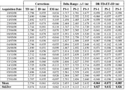
Corrections Delta Range-∆R(m) DR-TD+ET+ID (m)
Acquisition Date TD (m) ID (m) EM (m) PS-1 PS-2 PS-3 PS-1 PS-2 PS-3
10/02/08 2,796 0,055 -0,034 2,717 2,701 2,677 -0,058 -0,074 -0,098 03/03/08 2,690 0,066 0,016 2,541 2,552 2,532 -0,068 -0,057 -0,077 14/03/08 2,692 0,072 0,105 2,456 2,465 2,439 -0,059 -0,049 -0,076 25/03/08 2,655 0,074 -0,006 2,468 2,483 2,478 -0,119 -0,103 -0,109 05/04/08 2,744 0,081 -0,118 2,747 2,733 2,720 -0,033 -0,048 -0,061 27/04/08 2,780 0,072 0,070 2,597 2,585 2,547 -0,041 -0,053 -0,092 08/05/08 2,764 0,078 0,035 2,551 2,529 2,520 -0,100 -0,122 -0,131 30/05/08 2,803 0,073 -0,044 2,755 2,758 2,747 -0,019 -0,016 -0,027 24/07/08 2,916 0,056 -0,033 2,827 2,808 2,805 -0,067 -0,086 -0,089 04/08/08 2,796 0,055 -0,055 2,694 2,635 2,648 -0,102 -0,162 -0,149 26/08/08 2,890 0,051 -0,099 2,867 2,852 2,850 -0,071 -0,086 -0,088 06/09/08 2,888 0,056 -0,073 2,814 2,820 2,811 -0,091 -0,085 -0,095 11/11/08 2,712 0,048 -0,048 2,635 2,639 2,655 -0,077 -0,073 -0,057 22/11/08 2,653 0,064 0,003 2,545 2,515 2,513 -0,041 -0,071 -0,073 03/12/08 2,686 0,060 -0,050 2,606 2,627 2,593 -0,071 -0,049 -0,083 14/12/08 2,725 0,056 -0,113 2,727 2,723 2,714 -0,055 -0,059 -0,068 25/12/08 2,746 0,052 -0,034 2,680 2,707 2,674 -0,048 -0,021 -0,054 05/01/09 2,696 0,048 0,072 2,561 2,519 2,491 -0,015 -0,057 -0,085 16/01/09 2,737 0,048 0,026 2,568 2,587 2,560 -0,095 -0,076 -0,103 27/01/09 2,707 0,055 -0,097 2,701 2,654 2,660 -0,048 -0,096 -0,089
Mean 2,754 0,061 -0,024 2,653 2,645 2,632 -0,064 -0,072 -0,085
Std.Dev 0,074 0,010 0,062 0,115 0,113 0,117 0,027 0,032 0,026
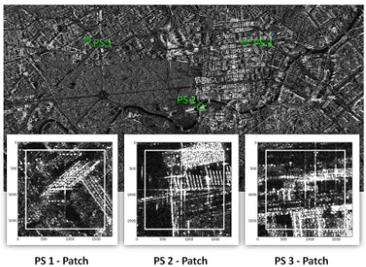
Figure 3: TSX Image of Berlin and the PS’s position and patches
Acquisition Mean inc. Resution date angle [deg] Azimuth x Range [m]
Image for Radargrammetric model
14/08/2008 50.95 1.1 x 0.45
Repeat pass image stack from 10/02/2008 form 29.99
1.1 x 0.45 to 27/01/2009 to 30.04
Table 1: Berlin TSX test site images features
has an ellipsoidal elevation of 144 m, around 65 m higher than the Berlin city and it is far around 30 km from Berlin.
For the experiment we have selected three different stable PS’s in one of the available images (see figure 3) and we have sup-posed that this points are not affected by a remarkable displace-ment (δ= 0) during the entire acquisition period (about one year from 02/2008 to 01/2009). The PS positions has been estimated using the described stereo approach and the results are reported in Table 2; for each of the three selected PS’s the standard devi-ation is less than 10 cm for the X component and is about 20 cm for the Y and Z components.
Theǫvalues obtained applying the described methodology are reported in the Table 3. As shown the residual errors for all the PS’s have a standard deviation of about 3 cm and a bias well be-low than 10 cm. Moreover the trends for each PS observed in the acquisition period has been investigated and are reported in the Fig. 4; it is clearly visible the quite good correlation between the
trends (min CC of 0.72 and max CC of 0.82) that is probably due both to orbit errors and to the not totally modelled atmospheric and geophysical effects.
Figure 4:ǫresiduals
6. CONCLUSION
position-ing accuracy of well identifiable and stable Persistent Scatterers (PS’s) along the SAR line of sight.
The PS absolute position has been computed using a stereo ap-proach and the necessary PS image coordinates has been retrieved using an automatic matching procedure. Starting from the posi-tions of PS and SAR satellite when imaging the PS itself (it can be computed by orbital information supplied into the metadata), it is possible to easily compute their distance and to compare it with the slant-range distance measured by the SAR sensor. The sig-nal propagation delays through the troposphere and ionosphere and the known geophysical effects inducing periodic and secular ground displacements have been considered in order to remove these phenomena from the distances measurements.
The available imagery used for the experiments on Berlin (Ger-many) test site are a repeat pass TerraSAR-X stack of 20 High resolution SpotLight images acquired from 2008 and 2009, with a mean incidence angle close to 30 degrees and one single image acquired with a mean incidence angle close to 50 degrees. Three different and stable PS’s have been selected and the results ob-tained show that it is possible to achieve a slant-range positioning accuracy with a bias well below 10 cm and a standard deviation of about 3 cm.
In the future this methodology could be conveniently adopted to monitoring deformation phenomena affecting both extended nat-ural areas and localized man-made structures.
ACKNOWLEDGEMENTS
TerraSAR-X imagery were made available, by Prof Sorgel Uwe, “Leibniz” University of Hannover (Germany), under the frame-work of a ISPRS Project: Evaluation of DEM derived from Terra-SAR-X
REFERENCES
Balss, U., Gisinger, C., Cong, X., Eineder, M. and Brcic, R., 2013. Precise 2-d and 3-d ground target localization with terrasar-x. International Archives of the Photogrammetry, Remote Sens-ing and Spatial Information Sciences XL-1/W1, pp. 23–28.
Berardino, P., Fornaro, G., Lanari, R. and Sansosti, E., 2002. A new algorithm for surface deformation monitoring based on small baseline differential sar interferograms. IEEE Transactions on Geoscience and Remote Sensing 40(11), pp. 2375–2383.
Bonafoni, S., Mazzoni, A., Cimini, D., Montopoli, M., Pierdicca, N., Basili, P., Ciotti, P. and Carlesimo, G., 2013. Assessment of water vapor retrievals from a gps receiver network. GPS Solu-tions 17(4), pp. 475–484.
Capaldo, P., Nascetti, A., Porfiri, M., Pieralice, F., Fratarcangeli, F., Crespi, M. and Toutin, T., 2014. Evaluation and comparison of different radargrammetric approaches for digital surface models generation from cosmo-skymed, terrasar-x, radarsat-2 imagery: Analysis of beauport (canada) test site. ISPRS Journal of Pho-togrammetry and Remote Sensing.
Cong, X., Balss, U., Eineder, M. and Fritz, T., 2012. Imag-ing geodesycentimeter-level rangImag-ing accuracy with terrasar-x: An update. IEEE TRANSACTIONS ON GEOSCIENCE AND RE-MOTE SENSING 9(5), pp. 948–952.
Eineder, M., Minet, C., Steigenberger, P., Cong, X. and Fritz, T., 2011. Imaging geodesy - toward centimeter-level ranging ac-curacy with terrasar-x. IEEE Transactions on Geoscience and Remote Sensing 49(2), pp. 661–671.
Klobuchar, A. and John, A., 1987. Ionospheric time-delay al-gorithm for single-frequency gps users. IEEE Transactions on Aerospace and Electronic Systems AES-23(3), pp. 325–331.
Leberl, F. W., 1990. Radargrammetric image processing. Artec House, Norwood MA.
McCarthy, D. and Petit, G., 2003. Iers conventions. IERS Tech-nical Note 32, Verlag des Bundesamts fur Kartographie und Geo-dasie Frankfurt am Main 2004.
Nascetti, A., Capaldo, P., Porfiri, M., Pieralice, F., Fratarcangeli, F., Benenati, L. and Crespi, M., 2014. Fast terrain modelling for hydrogeological risk mapping and emergency management: the contribution of high-resolution satellite sar imagery. Geomatics, Natural Hazards and Risk.
NATO, 1997. Stanag 4294: Navstar global positioning system (gps) c system characteristics - draft issue n, dated 1 may 1991.