VERTICAL VEGETATION STRUCTURE ANALYSIS AND HYDRAULIC ROUGHNESS
DETERMINATION USING DENSE ALS POINT CLOUD DATA – A VOXEL BASED
APPROACH
Michael Vettera,b*, Bernhard Höflec, Markus Hollausb, Christine Gschöpfa,d, Gottfried Mandlburgerb, Norbert Pfeiferb, Wolfgang Wagnera,b
aCentre for Water Resource Systems, Vienna University of Technology, 1040 Vienna, Austria - [email protected] [email protected], [email protected]
bInstitute of Photogrammetry and Remote Sensing, Vienna University of Technology, 1040 Vienna, Austria – mh,gm,[email protected]
cInstitute of Geography, University of Heidelberg, 69120 Heidelberg, Germany - [email protected]
dInstitute of Hydraulic Engineering and Water Resources Management, Vienna University of Technology, 1040 Vienna, Austria
Commission V, WG V/3
KEY WORDS:surface roughness, hydraulic simulation, Manning’sn, land cover, full-waveform, LiDAR
ABSTRACT:
In this contribution the complexity of the vertical vegetation structure, based on dense airborne laser scanning (ALS) point cloud data (25 echoes/m2
), is analyzed to calculate vegetation roughness for hydraulic applications. Using the original 3D ALS point cloud, three levels of abstractions are derived (cells, voxels and connections) to analyze ALS data based on a 1x1m2
raster over the whole data set. A voxel structure is used to count the echoes in predefined detrended height levels within each cell. In general, it is assumed that the number of voxels containing echoes is an indicator for elevated objects and consequently for increased roughness. Neighboring voxels containing at least one data point are merged together to connections. An additional height threshold is applied to connect vertical neighboring voxels with a certain distance in between. Thus, the connections indicate continuous vegetation structures. The height of the surface near or lowest connection is an indicator for hydrodynamic roughness coefficients. For cells, voxels and connections the laser echoes are counted within the structure and various statistical measures are calculated. Based on these derived statistical parameters a rule-based classification is developed by applying a decision tree to assess vegetation types. Roughness coefficient values such as Manning’snare estimated, which are used as input for 2D hydrodynamic-numerical modeling. The estimated Manning’s values from the ALS point cloud are compared with a traditional Manning’s map. Finally, the effect of these two different Manning’sn
maps as input on the 2D hydraulics are quantified by calculating a height difference model of the inundated depth maps. The results show the large potential of using the entire vertical vegetation structure for hydraulic roughness estimation.
1 INTRODUCTION
Airborne Laser Scanning (ALS), often referred to as LiDAR, is used as a fast and accurate technique to collect topographic infor-mation. ALS has become a state-of-the-art data source for cap-turing terrain data. ALS is a time and cost-effective method to acquire large area topographic data with low amount of user in-teraction, high ground sampling density and height accuracy of less than 15 cm. It is used for area-wide 3D data acquisition to support a range of scientific disciplines like (geo)archeology, geology, geomorphology, hydrology and many more (Höfle and Rutzinger, 2011).
Hydrology and water management benefit mostly from techno-logical advances in airborne, mobile and terrestrial laser scan-ning. It is a permanent process that sensor weight and size con-tinue to decrease whereas the functionality (full-waveform, mul-tiple pulses in air, mulmul-tiple wavelengths, on-line radiometric cal-ibration, higher sampling density, increasing vertical resolution etc.) and the usability are improving (Pfennigbauer and Ullrich, 2010). Because laser pulses can penetrate the vegetation canopy only through gaps of the foliage, a very dense ALS data set is needed to determine vertical vegetation structure parameters. Dense laser scanning point cloud data provide precise geome-try and high vertical resolution allowing an improved 3D surface classification for hydraulic roughness map calculation.
The roughness of the terrain and the type of vegetation (trees, shrubs or grass) have a strong influence on the floodplain and
channel flow regime. Thus, hydraulic models need to parameter-ize the effect of roughness through the use of hydraulic friction coefficients such as Manning’snor Chézy’sC, which describe the resistance of the channel and floodplain to the flow of water (Acrement and Schneider, 1984; Straatsma and Baptist, 2008). The state-of-the-art in hydraulic roughness parametrization is to use land cover maps derived from aerial images and/or field trips to estimate representative roughness values that show the most re-alistic flood inundation patterns. As highlighted in literature this method is not optimal because of the deficits in the model scheme and computation method. The model input may be compensated by using roughness values that are physically not representative (Straatsma and Baptist, 2008).
2 BACKGROUND
2.1 Vegetation structure and surface roughness
Remote sensing has been applied for Earth observation since the 1950s. The introduction of multi-echo LiDAR technology at the end of the 1990s, made simultaneous measurements of the canopies, inside the vegetation and the Earth surface under the vegetation possible. A huge community related to forestry using LiDAR data has been established in the last two decades. The main objectives are in the fields of mapping forested areas, detec-tion of vegetadetec-tion in urban areas, biomass calculadetec-tion, species dif-ferentiation and many others (Hyyppä et al., 2004; Naesset et al., 2004; Rutzinger et al., 2008; Höfle and Hollaus, 2010; Jochem et al., 2010). In forestry applications the use of the point cloud and the nDSM (normalized Digital Surface Model) is dominant. Since a few years an increasing number of studies make use of radiometric information together with the 3D point cloud from discrete echo recording or full-waveform (FWF) signal analysis or rasterized data with additional attributes for segmentation or classification approaches (Koch, 2010). The use of FWF tech-nology increases the ability to map vegetation in a more dense horizontal and vertical structure than with discrete echo record-ing systems (Doneus et al., 2010).
Fisher et al. (2009) use a voxel based approach to estimate the vegetation types in a semiarid region by deriving point density in different height levels. Hollaus et al. (2011), Hollaus and Höfle (2010) and Aubrecht et al. (2010) present new methods for es-timating vertical vegetation structure parameters of forested and urban areas using detrended terrain points (ALS) for plane fitting to describe the vertical distribution of ALS points per raster cell. By calculating the vertical vegetation structure it is possible to es-timate the volume of vegetation in different layers above the ter-rain (Hollaus et al., 2011). The studies of Hollaus et al. (2011), Aubrecht et al. (2010) and Hollaus and Höfle (2010) show the ability of accurate close-surface vegetation structure data extrac-tion.
An accurate DTM and roughness data are of high importance to simulate water flow characteristics. Due to recent developments in sensor technology, current ALS systems provide more infor-mation such as vertical resolution, point density, which can be used to generate more accurate DTMs (Pfennigbauer and Ullrich, 2010).
By using radiometric attributes of either discrete echo recording or FWF-sytems vegetation mapping can be improved (Höfle et al., 2009; Vetter et al., 2011). An additional attribute derived from the FWF signal is the ’echo width’, which is a measure of the height variation of a single echo within the laser footprint (Hollaus et al., 2011).
2.2 LiDAR used in hydraulics and hydrology
An extensive overview about active and passive remote sensing techniques in river environments is given by Marcus (2010), in which the main focus is on the water course. From a LiDAR per-spective three main topics are relevant for hydraulic studies: (i) the extent of the water surface, (ii) the digital elevation or terrain data of the river bed and the inundation area and (iii) the riparian vegetation, artificial objects (e.g. buildings) within the inundation area and roughness parameter delineation.
Höfle et al. (2009) and Vetter et al. (2009) present methods to extract the water surface extent from the ALS point cloud using radiometric and geometric information to map the water course.
Heritage and Milan (2009) demonstrate a method using terres-trial laser scanner (TLS) data to calculate the river bed roughness. Vetter et al. (2011) present a study about river bed model imple-mentation into the DTM by using terrestrially measured cross-section data to calculate the volume differences along the river bed caused by erosion and accumulation processes between two flood events.
Several studies are presented about DTM generation in general (Kraus and Pfeifer, 1998; Doneus et al., 2010). Related to hy-draulic simulations the main focus is on reducing the complexity of the DTM with minimum loss of information as presented in Mandlburger et al. (2009).
The used roughness term in hydraulic studies relates mainly to Manning’s or other empirical equations, in which the roughness value is used to describe the loss of energy of the fluids occur from grain size (in the channel) and/or form parameters such as vegetation type (Naudascher, 1992). However, the term rough-ness is used differently in various scientific disciplines and spatial scales of interest. Roughness in hydraulics has a different mean-ing than roughness in remote sensmean-ing (Acrement and Schneider, 1984; Naudascher, 1992). The challenge is to define roughness in the sense of the related discipline and to describe the way of the derived parameters and establish standards. Beside the cross-discipline definition problem, even within the remote sens-ing community there are different meansens-ings of the term ’rough-ness’. While in microwave remote sensing a surface may appear smooth, the very same surface is rough for LiDAR, because of the different scales (i.e. wavelengths). Thus, it is also a scaling problem, which increases by getting a better spatial and vertical resolution. Therefore, roughness should be related to the scale or spatial resolution of the data and the application or discipline (Hollaus et al., 2011).
Related to hydraulic roughness, vegetation and type of land cover have an significant influence on the output of hydrodynamic mod-eling. Many studies use ALS data for land cover mapping and vegetation classification for hydrodynamic models (Straatsma and Baptist, 2008; Alexander et al., 2010; Hollaus et al., 2011). Forested and flood inundated areas are covered by trees, shrubs and grass, which influence the flow characteristics of water, rep-resented by a distinct Manning value for each land cover class. By using ALS data the hydraulic friction coefficients for each vegetation cover type can be derived and used as input for 2D hydrodynamic-numerical models. Straatsma and Baptist (2008) present a workflow to calculate hydrodynamic relevant vegetation parameters for 2D hydrodynamic models from ALS data.
The state-of-the-art input data for flood modeling are: (i) the geometry provided as DTM of the watercourse (LiDAR, pho-togrammetry or terrestrial survey), (ii) roughness information, based on land cover maps which are produced from aerial im-ages or field trips, and (iii) the boundary conditions (water levels and/or discharge data).
Casas et al. (2010) present a workflow to estimate hydraulic rough-ness values using the∆Z value calculated from subtracting the DTM elevation from each laser echo within the related DTM cell. Finally, they use the DTM detrended laser echo height to estimate the off-terrain vegetation.
better vertical resolution via an increased digitizing rate of 1010 Hz (0.1 ns) (Pfennigbauer and Ullrich, 2010). Components of the surface roughness which are lower than the vertical resolu-tion of the used scanning system are contained in the recorded echo, which is also influenced by the terrain slope (Hollaus et al., 2011).
3 METHOD
The method focuses on hydraulic roughness estimation, where particularly roughness of the near surface layer is investigated. This approach demonstrates the possibility to map hydrodynamic-numerical roughness parameters such as Manning’snby using the ALS point cloud data. The main concept is to derive con-nected vertical vegetation structures and to use them as input for a rule-based classification to derive vegetation types, from which the Manning’sncan be derived.
3.1 General concept
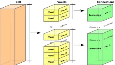
The main idea for delineating homogeneous roughness areas of surface-near vegetation is based on the spatial discretization of the laser echoes and an aggregation of the points into (a) cell-, (b) voxel- and (c) connection-level, which are the different spatial aggregation units (cf. Figure 1). We use this approach to calculate different levels of abstraction within a predefined search extent (1 x 1 m) to generate connected vertical vegetation structures.
Before sorting the echoes into the different aggregation levels the height of each echo is normalized to theZ0
level, which is the height of the DTM at the XY-position of the laser point. All addi-tional calculations are using this normalized height (nZ) values.
In a first step, all laser echoes are sorted into cells of 1 x 1 m size. In a second step, voxels are generated by slicing the cell into vertical height levels of equal height (0.5 m). Based on the
nZvalue each ALS echo is sorted into the related voxel. In a last step, vertically neighboring voxels are combined to larger units of arbitrary vertical extent (connections) where gaps between the voxels smaller than a predefined threshold (1.1 m) are ignored. Standard descriptive statistics (min, max, mean, median, std, ...) are derived for the cells, voxels and connections (18 parameters per level).
The statistical parameters of the cell-, voxel- and connection-levels serve as basis for a rule-based classification to derive vege-tation types, which are finally transferred to Manning values. It is assumed that the descriptive statistical values of the connections-level are significant parameters to derive hydraulic resistance val-ues.
Bare ground areas will contain only a single compact voxel/conn-ection per cell whereas vegetated areas are characterized by a larger vertical range of normalized height values within a cell. In the latter case, a certain number of occupied voxels per cell will be available. Depending on the vegetation structure, these voxels will be grouped together to one or more connections. The connections are a measure describing the compactness of the veg-etation, which can be used for roughness classification.
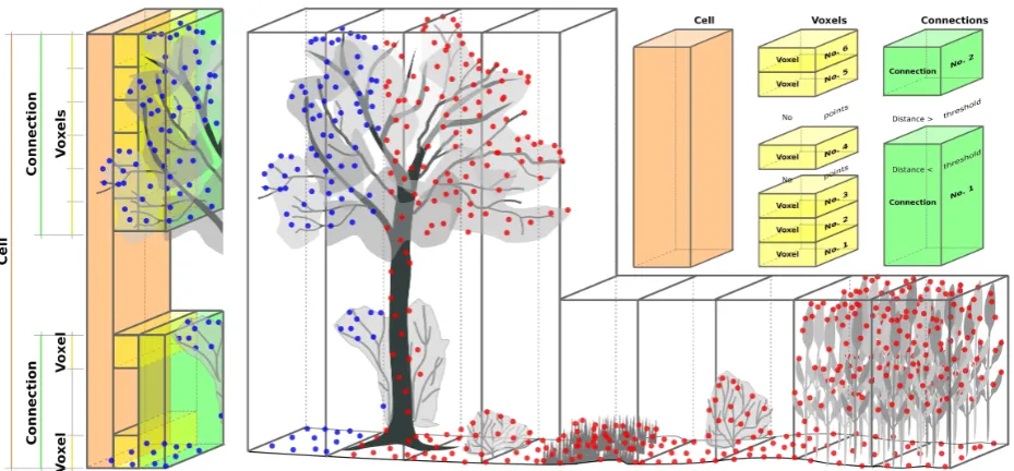
In Figure 1 and 2, the cell-, voxel- and connection-level abstrac-tion concept is demonstrated. First, the echoes per cell are col-lected, then the voxels are created and finally the vertical connec-tions are derived. In the right part of Figure 2 a schematic ALS point cloud is shown covering different vegetation types. The fur-thermost left part of Figure 2 represents all three levels at once for the cell with the blue echoes of the right generalized point cloud.
Figure 1: Basic concept: spatial discretization of the ALS point cloud into cell-level (a, left), voxel-level (b, middle) and connection-level (c, right)
The results are evaluated by visual comparison of the classifica-tion maps in Figure 3 as well as by comparing the hydrodynamic modeling results (depth and extent, Figure 4).
3.2 Cell-level
The cell-level is calculated in a X/Y domain of 1 x 1 m for the whole region, which is also the classification extent. Within each cell, the contained laser echoes are sorted by thenZvalue. The cell-level is the input for generating the voxels and can be used to classify forested areas using the maximum height.
3.3 Voxel-level
The Voxels represents a cube or a cuboid with either a regular or an irregular size. In this contribution the term voxel is used to describe a 3D bounding box. All echoes of the cell-level are sorted into the related voxels using thenZheights. The voxels are defined by the cell extent (X, Y) and the height of 0.5 m. Vox-els without any echo are erased and no longer used. The voxVox-els are used to generate the connected vertical structures by merging vertically neighboring voxels into single structures.
3.4 Connection-level
Connections describe vertically connected vegetation structures which are apparent in the ALS point cloud. In other words, the connections represent vegetation units or single plants. Connec-tions are derived by merging vertical neighboring voxels which are closer than a certain distance (1.1 m). This distance criterion is used to merge non illuminated areas which are assumed to be of the same vegetation structure as shown in the left part of Figure 2.
3.5 Hydraulic roughness classification
For hydraulic roughness classification as input data for a 2D hy-draulic simulation based on the ALS point cloud the statistical parameters of the cells, voxels and connections are used. Differ-ent roughness products can be generated by using a rule-based classification. Therefore, the surface-near vegetation roughness is important and used in the classification of the lowest connec-tion. For other roughness products like canopy roughness the upper connections are of interest.
Figure 2: Schema of the cell-, voxel- and connection-level related to a generalized ALS point cloud for different vegetation structures
Roughness class Rule-base Vegetation type
0.045 max. height(lowest connection) < 0.15 streets, short grassland 0.050 max. height(lowest connection) > 0.15 AND < 0.25 grassland, agricultural area 0.070 max. height(lowest connection) > 0.25 AND < 2.00 shrubs
0.090 max. height(lowest connection) > 2.00 AND < 5.00 reed 0.100 number of connections > 1 AND max. height(cell) < 10.00 small trees 0.125 number of connections > 1 AND max. height(cell) > 10.00 forest
Table 1: Rule-base for hydraulic roughness classification
Finally, the derived rule-base (decision tree) is applied to the ALS data using the statistical values shown in Table 1. After classi-fying the 1x1 m cells in to vegetation types and transferring to Manning’snvalues a modus filter with 8 neighbors is used to smooth the result and to reduce the spatial heterogeneity of the resulting classification raster.
With the presented method it is not possible to derive the related river bed roughness parameters. Therefore, the roughness val-ues are manually classified for areas that are covered by water. The water surface extents are delineated based on a DTM and an ALS intensity image by a raster-based classification of low ALS intensity values and a maximum DTM slope of less than2◦as described in Vetter et al. (2011).
4 RESULTS AND DISCUSSION
The results of the classification are shown in Figure 3(b). A visual evaluation of the results has been carried out between the classi-fied ALS and the traditionally derived Manning’snvalues in Fig-ure 3(a). As shown in FigFig-ure 3 the dominant spatial patterns of the Manning’s values are comparable. But the ALS derived val-ues represent the whole area in more detail than the traditionally derived map. Major differences are predominantly characterized by the neighboring Manning classes in the ALS derived data. Be-tween class 0.045 and 0.050 or 0.100 and 0.125 large differences are evident, which we assume that they occur from wrong clas-sification rules due to the low overall accuracy of 65% for those four classes. For all other classes the overall accuracy is better than 90%.
Furthermore, the hydrodynamic modeling results (depth and area of inundation) are compared by using both roughness maps as input. A calibrated model was used to perform two simulations
with the same boundary conditions and the same DTM input data with both roughness maps (original and ALS derived). Differ-ences of the two simulation results are in the range of 2 to 3 cm in water depth and a difference in inundation area extent of less than 2800m2
(< 1% of total inundated area, Figure 4).
The roughness classification rules are based on a decision tree using a subsample of the ALS data with calculated voxel and connection statistical values (ALS derived) created from the orig-inal Manning’snmap. These results in already calibrated Man-ning’snvalues for the classification of the connections where the derived roughness map can be used as input for the 2D simula-tion without any further calibrasimula-tion. If no calibrated reference data are available, the calibration effort is the same as with tradi-tional data. But the advantage of using ALS data for roughness estimation is the standardization and transferability of the classifi-cation and therefore the reduction of manual classificlassifi-cation errors. The second benefit is that the calculation is performed fully auto-matically without any user interaction. The main potential of the proposed method is to reach one consistent input data set for the geometry and roughness data (elevation and Manning’sn) both derived from ALS data originating from one date of acquisition. Which is not the case if different land use and land cover data are used to produce Manning’snmaps from different sources as it is state-of-the-art up to now.
5 CONCLUSIONS AND FUTURE WORK
(a) Traditionally derived Manning’s values
(b) ALS derived Manning’s values
Figure 3: Traditionally derived Manning’s values vs. the ALS derived values[s/m1/3
]
of detail clearly increases by the use of the proposed method, as well as having only little effects on the 2D hydraulic sim-ulation results (water depth and inundated extent). Therefore, we assume that this method is applicable to produce hydraulic roughness maps, which base on geometry data. The low differ-ences between the two hydrodynamic model results lead us to the conclusion that the spatial distribution of the Manning’s values in our study is a feature with low impact on the hydraulic mod-eling results. However, Manning’snis an empirical value, the transfer of the ALS based method to other regions can be prob-lematic. We assume that a more physically founded parameter such as the Darcy-Weissbach valuefperforms better. Therefore, some further tests should be done with the presented method to identify the roughness value that can be described best by ALS geometry data. A further approach is to use the FWF echo width and backscatter information to improve classification results es-pecially for smooth areas such as roads and short grassland.
The presented approach does not include the slope effect for the normalized height value calculation, which results in overestima-tion of the height value. This results in misclassificaoverestima-tion in areas with steep slopes which were not evident in the used test site. By applying a slope adaptivenZvalue the classification is made free of slope effects and should finally result in better classifica-tion accuracy.
One important feature of the approach is the point density which has yet to be investigated. The proposed method uses statistical values per cell, voxel and connection and we assume the point
(a) Inundation depth from ALS derived Manning’sn(Q = 5000m3
/s)
(b) Depth difference from ALS – traditional 2D simulation
Figure 4: Depth of inundated area and difference model from 2D simulation based on the same boundary conditions for ALS and traditional derived Manning’sn[m]
density is an important affecting parameter. It should be possible to derive an inundation depth dependent hydraulic friction coef-ficient by using the connection-level values in different heights.
References
Acrement, G. and Schneider, V., 1984. Guide for selecting man-ning’s roughness coefficients for natural channels and flood-plains. Report FHWA-TS-84-204, U.S. Department of Trans-portation, Federal Highways Administration.
Alexander, C., Tansey, K., Kaduk, J., Holland, D. and Tate, N., 2010. Backscatter coefficient as an attribute for the classifi-cation of full-waveform airborne laser scanning data in urban areas. ISPRS Journal of Photogrammetry and Remote Sensing 65(5), pp. 423–432.
Aubrecht, C., Höfle, B., Hollaus, M., Köstl, M., Steinnocher, K. and Wagner, W., 2010. Vertical roughness mapping - als based classification of the vertical vegetation structure in forested areas. In: The International Archives of the Photogramme-try, Remote Sensing and Spatial Information Sciences, Vol. XXXVIII-7B, Vienna, Austria, pp. 35–40.
Casas, A., Lane, S., Yu, D. and Benito, G., 2010. A method for parameterising roughness and topographic sub-grid scale effects in hydraulic modelling from lidar data. Hydrology and Earth System Sciences 14(8), pp. 1567–1579.
Doneus, M., Briese, C. and Studnicka, N., 2010. Analysis of full-waveform als data by simultaneously acquired tls data: To-wards an advanced dtm generation in wooded areas. In: In-ternational Archives of Photogrammetry, Remote Sensing and Spatial Information Sciences, Vol. XXXVIII-7B, Vienna, Aus-tria, pp. 193–198.
Fisher, J., Erasmus, B., Witkowski, E., van Aardt, J., Asner, G., Kennedy-Bowdoin, T., Knapp, D., Emerson, R., Jacobson, J., Mathieu, R. and Wessels, K. J., 2009. Three-dimensional woody vegetation structure across different land-use types and -land-use intensities in a semi-arid savanna. In: IGARSS (2)’09, pp. 198–201.
Heritage, G. L. and Milan, D., 2009. Terrestrial laser scanning of grain roughness in a gravel-bed river. Geomorphology 113(1-2), pp. 4–11.
Höfle, B. and Hollaus, M., 2010. Urban vegetation detection us-ing high density full-waveform airborne lidar data - combina-tion of object-based image and point cloud analysis. In: The International Archives of the Photogrammetry, Remote Sens-ing and Spatial Information Sciences, Vol. XXXVIII-7B, Vi-enna, Austria, pp. 281–286.
Höfle, B. and Rutzinger, M., 2011. Topographic airborne LiDAR in geomorphology: A technological perspective. Zeitschrift für Geomorphologie/Annals of Geomorphology 55(2), pp. 1–29.
Höfle, B., Vetter, M., Pfeifer, N., Mandlburger, G. and Stötter, J., 2009. Water surface mapping from airborne laser scanning using signal amplitude and elevation data. Earth Surface Pro-cesses and Landforms 34(12), pp. 1635–1649.
Hollaus, M. and Höfle, B., 2010. Terrain roughness parameters from full-waveform airborne lidar data. In: The International Archives of the Photogrammetry, Remote Sensing and Spa-tial Information Sciences, Vol. XXXVIII-7B, Vienna, Austria, pp. 287–292.
Hollaus, M., Aubrecht, C., Höfle, B., Steinnocher, K. and Wag-ner, W., 2011. Roughness mapping on various vertical scales based on full-waveform airborne laser scanning data. Remote Sensing 3(3), pp. 503–523.
Hyyppä, J., Hyyppä, H., Litkey, P., Yu, X., Haggrén, H., Rönnholm, P., Pyysalo, U., Pitkänen, J. and Maltamo, M., 2004. Algorithms and methods of airborne laser scanning for
forest measurements. In: International Archives of Photogram-metry, Remote Sensing and Spatial Information Sciences, Vol. XXXVI-8/W2, pp. 82–89.
Jochem, A., Hollaus, M., Rutzinger, M., Höfle, B., Schadauer, K. and Maier, B., 2010. Estimation of aboveground biomass us-ing airborne lidar data. In: Proceedus-ings of Silvilaser 2010, the 10th International Conference on LiDAR Applications for As-sessing Forest Ecosystems, Freiburg, Germany. digital media.
Koch, B., 2010. Status and future of laser scanning, synthetic aperture radar and hyperspectral remote sensing data for for-est biomass assessment. ISPRS Journal of Photogrammetry and Remote Sensing 65(6), pp. 581 – 590. ISPRS Centenary Celebration Issue.
Kraus, K. and Pfeifer, N., 1998. Determination of terrain models in wooded areas with airborne laser scanner data. ISPRS Jour-nal of Photogrammetry and Remote Sensing 53(4), pp. 193– 203.
Mandlburger, G., Hauer, C., Höfle, B., Habersack, H. and Pfeifer, N., 2009. Optimisation of LiDAR derived terrain models for river flow modelling. Hydrology and Earth System Sciences 13, pp. 1453–1466.
Marcus, W., 2010. Remote sensing of the hydraulic environment in gravel bed rivers. In: 7th Gravel-Bed Rivers Conference 2010, Tadoussac, Québec.
Naesset, E., Gobakken, T., Holmgren, J., Hyyppä, H., Hyyppä, J., Maltamo, M., Nilsson, M., Olsson, H., Persson, A. and Soder-man, U., 2004. Laser scanning of forest resources: the nordic experience. Scandinavian Journal of Forest Research 19(6), pp. 433–442.
Naudascher, E., 1992. Hydraulik der Gerinne und Gerinnebauw-erke. 2. Springer Verlag, Wien, New York.
Pfennigbauer, M. and Ullrich, A., 2010. Improving quality of laser scanning data acquisition through calibrated amplitude and pulse deviation measurement. In: Proc. SPIE, Vol. 7684-76841F.
Rutzinger, M., Höfle, B., Hollaus, M. and Pfeifer, N., 2008. Object-based point cloud analysis of full-waveform airborne laser scanning data for urban vegetation classification. Sensors 8(8), pp. 4505–4528.
Straatsma, M. and Baptist, M., 2008. Floodplain roughness parameterization using airborne laser scanning and spectral remote sensing. Remote Sensing of Environment 112(3), pp. 1062–1080.
Vetter, M., Höfle, B. and Rutzinger, M., 2009. Water classifica-tion using 3D airborne laser scanning point clouds. Österre-ichische Zeitschrift für Vermessung & Geoinformation 97(2), pp. 227–238.
Vetter, M., Höfle, B., Rutzinger, M. and Mandlburger, G., 2011. Estimating changes of riverine landscapes and riverbeds by us-ing airborne lidar data and river cross-sections. Zeitschrift für Geomorphologie/Annals of Geomorphology 55(2), pp. 51–65.
ACKNOWLEDGEMENTS
![Figure 4: Depth of inundated area and difference model from 2Dsimulation based on the same boundary conditions for ALS andtraditional derived Manning’s n [m]](https://thumb-ap.123doks.com/thumbv2/123dok/3225802.1395789/5.595.64.546.76.444/inundated-difference-dsimulation-boundary-conditions-andtraditional-derived-manning.webp)
