MULTI-MODAL REMOTE SENSING DATA FUSION FRAMEWORK
M. A. A. Ghaffar a, T. T. Vu a,c, T. H. Maul b
a School of Environmental and Geographical Sciences, University of Nottingham, Malaysia campus -(khgx4mad,[email protected])
b School of Computer Science, University of Nottingham, Malaysia campus - ([email protected])
c
Faculty of Science and Engineering, Hoa Sen University, Vietnam
Commission IV, WG IV/4
KEY WORDS: Deep Learning, Convolutional Neural Networks, Super resolution, Crowd-sourced data, Data fusion
ABSTRACT:
The inconsistency between the freely available remote sensing datasets and crowd-sourced data from the resolution perspective forms a big challenge in the context of data fusion. In classical classification problems, crowd-sourced data are represented as points that may or not be located within the same pixel. This discrepancy can result in having mixed pixels that could be unjustly classified. Moreover, it leads to failure in retaining sufficient level of details from data inferences. In this paper we propose a method that can preserve detailed inferences from remote sensing datasets accompanied with crowd-sourced data. We show that advanced machine learning techniques can be utilized towards this objective. The proposed method relies on two steps, firstly we enhance the spatial resolution of the satellite image using Convolutional Neural Networks and secondly we fuse the crowd-sourced data with the upscaled version of the satellite image. However, the covered scope in this paper is concerning the first step. Results show that CNN can enhance Landsat 8 scenes resolution visually and quantitatively.
1. INTRODUCTION
The current improvements in remote sensing data resolution provides more variety of choices in extracting meaningful information for different kinds of remote sensing applications. Not only the most appropriate resolution can be obtained, but also the fusion between different resolutions is enabled to produce better outcomes. Utilizing from these improvements, remote sensing scientists have developed numerous algorithms (Padarian et al. 2015) (Wu 2016) (Camps-Valls 2009) to extract features, objects and patterns that helped in data interpretation and analysis operations. However, most of the followed methodologies were developed originally to fit with the recently launched satellites e.g. WorldView-2, 3 and 4 or Quickbird . (Gueguen et al. 2017) (Johnson et al. 2013) which are producing very high resolution satellite images.
Considering global land cover applications, the majority of the products which available nowadays are using low resolution e.g. GLC2000 (JRC 2015) and MODIS in order to cover huge areas which results in inaccurate results in some cases (See et al. 2015). The ongoing movement towards producing higher resolution global landcover maps is trying to fill the gap of the accuracy and produce an overall enhanced products which will take land cover maps to the next level.
However, whether used in training or as a reference dataset, ground data is still critical for remote sensing data processing algorithms. Insufficient ground data has been the big issue in remote sensing data processing. Therefore, even though adopting various advanced image processing techniques, remote sensing data analysis still requires lots of human interaction and the level of automation remains low. Concurrently, crowd-sourced data arose as an auxiliary factor that can provide support to the developed algorithms (Ahmed et al. 2015) (Fritz et al. 2012) (Schmitt & Zhu 2016) as an additional source of information for enhancing/evaluating the results.
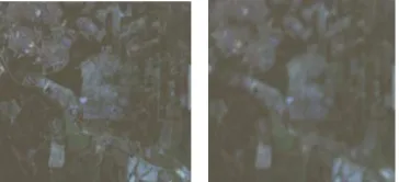
Nevertheless, the inconsistency between the freely available remote sensing datasets and crowd-sourced data resolutions forms a big challenge in the context of data fusion. In classical classification problems, crowd-sourced data are represented as points that may be or not located within the same pixel. This discrepancy can result in having mixed pixels that could be unjustly classified which leads to the failure in retaining sufficient level of details from data inferences (See Fig.1)
Since it is difficult to update the attached sensors on the launched satellites, post-processing is the most attainable option that could be achieved to enhance spatial resolution. Research and development efforts were going towards finding solutions that can bring out the best of the freely available data sources altogether.
Artificial intelligence is one of the computer science specializations that attempts to model all facets of human intelligence (Russell et al. 1995) . As a sub-field, Machine Learning (ML) is concerned with creating systems that can adapt to different situations/problems and giving the computers the ability to think by learning. Machine learning algorithms have been used in many applications such as computer vision, natural language processing, speech recognition, and remote sensing also. Due to the complexity of information contained in remote sensing scenes, which demands massive training dataset, the use of machine learning for remote sensing image analysis is still at the early stage. However, the increase of access to free medium-low resolution satellite imagery motivated remote sensing scientists to find advanced processing techniques that can help in enhancing satellite images spatial resolution.
process of the detailed sub-pixel level in the super-resolved image.
Figure 1. Single Landsat 8 pixel 30x30m that contains tens of crowd-sourced data points (Blue=>water,
Green=> vegetation, Red=>built-up) and all resides within same pixel which leads to confuse the
classifier and gives false predicted values.
Several Super-Resolution techniques gained attention mostly from computer scientists (Dong et al. 2015) (Bevilacqua et al. 2012) (Hong Chang et al. 2004) yet to have the same from remote sensing communities. Some recent research done on remote sensing data e.g. (Al-shabili et al. 2015) but still focusing on gray scale images and didn't provide ground truth images to be used in comparison to the up-scaled results. While (Huang et al. 2015) applied DNN “Deep Neural Networks” for pansharpening purpose by learning the high resolution features from the panchromatic bands available from commercial satellites such as Ikonos and Quickbird and MS “Multi Spectral ” containing RGB and NIR “Near InfraRed”.
In this paper, we adopt the super-resolution algorithm written by (Dong et al. 2015) which is developed originally for non-satellite images. The contribution here is modifying the algorithm to work with high dimensional remote sensing datasets and retaining the state-of-the-art performance with smaller training datasets. The structure of the paper is as follows: In Section II, we describe super-resolution state-of-the-art techniques available right now with focus on the example based methodologies. We then give a detailed explanation of the followed methodology and the processing phases we carried “High Resolution” image from LR “Low Resolution” images. (Yang et al. 2015). This technique is breaking through the limitation of updating the attached imaging sensors on the launched satellites. Back to 1960s, (Harris 1964) was the pioneer in constructing HR image from a LR one. After some time, SR became more sophisticated and developed with innovative approaches of inferring the HR details from the LR input. During 1980s, (Huang & Tsay 1984) enhanced the resolution of scenes received from Landsat TM satellite. Until recently, (Romano et al. 2016) , (Dong et al. 2016) and (Dong et al. 2015) the trend of SR evolved totally towards the example-based methods. Example-based methods use a
dictionary of mapping between LR and HR to infer the unknown HR details (Bevilacqua et al. 2012) It exploits the self-similarity and generate patches from the input images.
2.1 Super-Resolution Convolutional Neural Network
(SRCNN)
Convolutional Neural Networks “CNN” are inspired by the biological brain. It simulates the way of thinking that human brain is using to identify or recognize any patterns (Arbib 2003). Given that training dataset incorporates X and Y, X represents the synthesized LR patches while Y is the HR (original) patches. (Dong et al. 2015) used CNN to learn constructing a HR image from the LR patches coming from the training dataset. This operation has 3 phases/layers as follows:
2.1.1 Patch extraction: The first layer designed to extract features from the input patches according to a 9x9 convolution (filtering) process. The filter (aka kernel) here is created with initiated random values that represent pixel's weight. These weights are to be changed according to the importance of the feature to be extracted. In order to extract the features, we slide the filter over the input image patch (64x64) by one pixel a time (stride). Matching pixel per pixel from the input image and the kernel, multiplication is done first before we accumulate the total from multiplication and divide it by 81 which is 9x9 (the number of pixels in the kernel). This process is done per band per feature. At the end of this step, feature maps created for all the input images and ready to be passed to the second layer. After creating the convolution layer, an activation function is set to run over the feature map. ReLu or Rectified Linear Unit is one of the most used activation functions that represents the non-linearity in the model. Most of the real-world data that could be learnt from CNN are non-linear. Hence, ReLU is used to introduce non-linearity in the proposed model.
The first layer can be expressed in equation (1):
(1) F1(Y) = max(0,W1 Y+B1)∗
where W1 represents the filters B1 represents the biases
max(0,x) is the ReLu activation function
2.1.2 Non-linear mapping: Having the output from the first
layer as an input to the second layer, the second layer function is mapping the features from the low resolution input (feature maps from first layer) to another feature map that will be used for producing the high resolution image. This non-linear mapping is reducing the dimensionality of the data. Having 64 features from first layer, after mapping it to the high resolution data, only 32 features will be used to create the high resolution patches. These 32 features are the most efficient in constructing the final output in the third layer.
Second layer operation represented in equation (2):
(2) F2(Y) = max (0,W2 F1(Y)+B2)∗
where F1(Y) is the output (feature maps) from the first layer, W2 is the number of filters
B2 is 32dimensional bias
2.1.3 Output construction: The third layer is responsible of constructing the final output (high resolution image) after applying the last convolution process which takes the average of the overlapped pixels (from generated high resolution patches). The construction process achieved by converting the n2 B3 is the corresponding dimensional vector F2(Y) is the output feature maps from second layer
2.2 Landsat8 Super-resolution
In this section, the processing phases are discussed starting from data preparation till output construction.
2.2.1 Data preprocessing: Unlike SRCNN, preprocessing
step here is of vital importance. Before creating the training dataset, to avoid geometric distortions, geometric correction has to be achieved on the selected scenes. Moreover, very much alike any remote sensing data, there could be some missing pixel values or NO DATA for pixels. In this case, some of the machine learning techniques can ignore the missing values and others can replace the missing value with median value.
2.2.2 Dataset creation: At this phase, the chosen scenes need to be checked against any missing or corrupted values that have been obtained while capturing them. Moreover, as a very common issue with tropical areas, the captured scenes are always having cloud coverage that affects the quality of the final output. The selected scenes were filtered against the cloud coverage to get the least percentage of cloud (< 5%) via the continuously updated scenes list from AWS “Amazon Web Services” (AWS 2017). Following the rule of thumb in creating machine learning datasets, scenes are split into training and test sets. The selected scenes are path 126 and row 58 for training and 127,58 for validation which are covering Malaysia. Using fully open source libraries e.g. Gdal, QGIS, Fiona and Scipy, the training and validation datasets are created to reflect the SR objective. Patch extraction achieved by cropping 64x64 patches from training scene. To synthesize the LR patches, we applied Gaussian blur with .5 sigma, then sub-sample x2 and then up-scale x2 using Bicubic interpolation. While the HR patches will be a copy from the extracted patches without any processing. Figure 2 shows an example from the HR and LR patches. Our target is to train the model to retrieve the original image from the synthesized patches.
Figure 2. An example of HR 64x64 on the left and LR patch on the right after applying the Gaussian blur, sub-sampling and
up-scaling.
The created dataset contained 5000 64x64 patches with overlapping 8 pixels per patch then divided to training and
validation with 3500 and 1500 respectively. The validation test will be used to validate the model predictions of the HR output.
2.2.3 Training the model: As mentioned above, the model
has 3 layers that used to extract the features that can construct the HR output. However, unlike SRCNN, we have more channels/bands to be fed as input for the model. RGB is not sufficient enough when it comes to satellite images. Landsat8 has 11 bands to be utilized. We included the RGB in addition to the NIR, SWIR 1 and SWIR 2. The 6 bands are passed to the model layer by layer sequentially. The open source deep learning framework Theano has been used for the training process with 8 CPU cores and 16 GB RAM server running on Ubuntu OS.
The required processing time relies on many factors. The number of image patches “training dataset” and the number of extracted features affects how fast the processing can be done. We initiated the number of features to be extracted in the first layer to be 128 then 64 in the second layer. Also the average of time to complete a full presentation of the data “aka epoch” to be learned differs from 4 to 5 hours per epoch. We tested the model with 10 epochs which took around 2 days of processing the training and validation datasets.
3. RESULTS
In order to evaluate the model accuracy quantitatively, evaluation matrices like MSE (Mean Squared Error) function can compare the actual pixels values with the predicted ones. MSE is measuring the mean of the squares of the errors for those existing between estimator and the estimated values. However, to measure image restoration quality, MSE got one problem since it relies strongly on the pixel intensity. This leads to having inconsistent MSE values according to the bit depth of the images (Joshi et al. 2016). Hence, PSNR (Signal-to-Noise Ratio) is used as it scales the MSE according to the image range (Veldhuizen 2016) see equations 4 and 5. PSNR will compare between the original image and the generated one. In order to have a reference to compare our results with, testing the up-scale process will be done by downscaling the original image by factor of 2 then we use the model to up-scale it by same factor. Hence, PSNR could be calculated between the original and the up-scaled version of the image.
(4)
where ĝ(n,m) and g(n,m) are the two images
(5)
where S represents the maximum pixel value
Patches Training PSNR Validation PSNR
64x64 40.523 dB 39.112 dB
32x32 41.214 dB 41.003 dB
Table 1. Different patches training and validation scores of PSNR in dB
Table 1 shows that the achieved accuracy from the 32x32 patches was slightly higher than the 64x64 ones. However, it depends on the dimensions of the up-scaled output image and the representation of the image in the training samples. While figure 3 shows a visual comparison between the original image and the up-scaled one.
Figure 3.a: Example for 660x660 pixels original image
Figure 2.b: A 2x up-scaled version of the 330x330 pixels to match with 660x660 original image.
4. CONCLUSIONS
We have presented the first step of two steps framework that will help in increasing the automation level of satellite image understanding applications e.g. landcover maps. Example-based super-resolution methodology adopted to enhance Landsat 8 scenes with Deep Convolutional Neural Networks to infer details from image patches and generate HR output. Different model parameters need to be explored e.g. filter size, number of features and number of layers.
5. ACKNOWLEDGEMENT
This study is part of a project funded by FRGS, Malaysia Ministry of Education, grant no. FRGS/2/2013 /ICT07 /UNIM/02/1.
This work was supported by AWS in form of Education Grant award.
6. REFERENCES
Ahmed, M. et al., 2015. Crowd-2-cloud – remote sensing land cover verification with crowd-sourcing data. Free and Open Source Software for Geospatial.
Al-shabili, A., Taha, B. & Al-ahmad, H., 2015. Superresolution Algorithm for Satellite Still Images. , pp.48–51.
Arbib, M., 2003. The handbook of brain theory and neural networks.
AWS, 2017. Landsat on AWS. Amazon Web Services. Available at: https://aws.amazon.com/public-data-sets/landsat/ [Accessed October 1, 2015].
Bevilacqua, M. et al., 2012. Low-Complexity Single-Image Super-Resolution based on Nonnegative Neighbor Embedding. Procedings of the British Machine Vision Conference 2012, (Ml), pp.135.1–135.10.
Camps-Valls, G., 2009. Machine learning in remote sensing data processing. 2009 IEEE International Workshop on Machine Learning for Signal Processing, pp.1–6.
Dong, C. et al., 2015. Image Super-Resolution Using Deep Convolutional Networks. arXiv:1501.00092v2, pp.1–14.
Dong, C., Loy, C.C. & Tang, X., 2016. Accelerating the super-resolution convolutional neural network. Lecture Notes in Computer Science (including subseries Lecture Notes in Artificial Intelligence and Lecture Notes in Bioinformatics), 9906 LNCS, pp.391–407.
Fritz, S. et al., 2012. Geo-Wiki: An online platform for improving global land cover. Environmental Modelling & Software, 31, pp.110–123.
Gueguen, L. et al., 2017. Mapping Human Settlements and Population at Country Scale From VHR Images. , 10(2), pp.524–538.
Harris, J., 1964. Diffraction and Resolving Power*. J. Opt, 54, pp.931–936.
Huang & Tsay, R., 1984. Multiple frame image restoration and registration. In Advances in Computer Vision and Image Processing, 1, pp.317–339 .
Huang, W. et al., 2015. A New Pan-Sharpening Method With Deep Neural Networks. IEEE Geoscience and Remote Sensing Letters, 12(5), pp.1037–1041.
Johnson, B.A., Tateishi, R. & Hoan, N.T., 2013. A hybrid pansharpening approach and multiscale object-based image analysis for mapping diseased pine and oak trees. International Journal of Remote Sensing, 34(November), pp.6969–6982.
Joshi, K., Yadav, R. & Allwadhi, S., 2016. PSNR and MSE based investigation of LSB. 2016 International Conference on Computational Techniques in Information and Communication Technologies, ICCTICT 2016 - Proceedings, pp.280–285.
JRC, 2015. Global Land Cover 2000. EU. Available at: http://forobs.jrc.ec.europa.eu/products/glc2000/glc2000.php [Accessed June 1, 2017].Padarian, J., Minasny, B. & Mcbratney, a B., 2015. Computers & Geosciences Using Google ’ s cloud-based platform for digital soil mapping. Computers and Geosciences, 83, pp.80–88.
Romano, Y., Isidoro, J. & Milanfar, P., 2016. RAISR: Rapid and Accurate Image Super Resolution. , pp.1–31.
Russell, S.J. et al., 1995. Artificial Intelligence A Modern Approach, Library of Congress.
Schmitt, M. & Zhu, X.X., 2016. Data Fusion and Remote Sensing. IEEE GEOSCIENCE AND REMOTE SENSING MAGAZINE, (DECember).
See, L. et al., 2015. Building a hybrid land cover map with crowdsourcing and geographically weighted regression. ISPRS Journal of Photogrammetry and Remote Sensing, 103, pp.48– 56.
Veldhuizen, T., 2016. Measures of image quality. The Evolving, Distributed, Non-Proprietary, On-Line Compendium of Computer Vision.
Wu, Y., 2016. A simplified training data collection method for sequential remote sensing image classification. International Workshop on Earth Observation and Remote Sensing Applications, pp.14–17.
Yang, D. et al., 2015. Remote Sensing Image Super-resolution :