ACCURACY EVALUATION OF STEREO CAMERA SYSTEMS WITH GENERIC
CAMERA MODELS
Dominik Rueß, Andreas Luber, Kristian Manthey and Ralf Reulke
German Aerospace Center Rutherfordstraße 2 12489 Berlin-Adlershof, Germany
(Dominik.Ruess,Andreas.Luber,Kristian.Manthey,Ralf.Reulke)@dlr.de
Commission V/5
KEY WORDS:Reconstruction, Geometry, Accuracy, Generic Cameras, Camera Model, Wide Baseline
ABSTRACT:
In the last decades the consumer and industrial market for non-projective cameras has been growing notably. This has led to the de-velopment of camera description models other than the pinhole model and their employment in mostly homogeneous camera systems. Heterogeneous camera systems (for instance, combine Fisheye and Catadioptric cameras) can also be easily thought of for real appli-cations. However, it has not been quite clear, how accurate stereo vision with these cameras and models can be. In this paper, different accuracy aspects are addressed by analytical inspection, numerical simulation as well as real image data evaluation. This analysis is generic, for any camera projection model, although only polynomial and rational projection models are used for distortion free, Cata-dioptric and Fisheye lenses. Note that this is different to polynomial and rational radial distortion models which have been addressed extensively in literature.
For single camera analysis it turns out that point features towards the image sensor borders are significantly more accurate than in center regions of the sensor. For heterogeneous two camera systems it turns out, that reconstruction accuracy decreases significantly towards image borders as different projective distortions occur.
1 INTRODUCTION
Classical projective cameras have long been subject to stereo vi-sion. Camera self-calibration, automated relative orientation, stereo reconstruction and many more issues have been very successfully worked on. With the introduction of panoramic or wide angle cameras several models have been developed, which are able to cope with the non-projective nature of many of these types of cameras, some of which are several trigonometric models for Fisheye lenses and catadioptric projection models. To prevent having to use different camera models within one application of heterogeneous cameras, generic camera models like the polyno-mial model, division model, rational model and shifted sphere model have been introduced. Furthermore, some approaches to perform stereo reconstruction on different types of cameras have been suggested, resulting in particular Epipolar models yielding curves instead of Epipolar lines. The results of these contribu-tions quite often lack comprehensive investigacontribu-tions into recon-struction accuracy, as it is often required in photogrammetry. This paper investigates the whole process of 3D reconstruction with the above mentioned generic camera models. The main focus here is the influence of the radial distance to the projection cen-ter.
The next section will provide a short overview of existing ap-proaches and camera models. This will be followed by a short review on stereo computation used for this paper. Afterwards, the results of analytical, numerical and real image data tests will be presented and evaluated.
Throughout this paper two camera systems will be used. As for the naming convention, lower case letters~xwill describe image points, upper case lettersX~ are used for three dimensional ob-ject points and left-right image differentiation will be done with or without a hyphenx~′for the left and right image, respectively. The subscriptdwill describe an entity within the distorted do-main. If not stated differently, units are measured in millimeters.
2 CAMERA MODELS OVERVIEW
There are different models for describing the imaging geometry of a two camera system.
In Photogrammetry the imaging process can be modeled by means of the collinearity equations, see (Kraus, 2004). A world pointX~ is mapped to an image point by subtracting the camera centerC~ first, followed by rotating with the orientation matrixR. This in-cludesc, the focal length andx0,y0are the camera center offset.
The resulting image vector~xdescribes to location on the sensor.
2.1 Radial Distortion
This model describes the imaging process of distortion free cam-eras very accurately. It is also known as thepinhole model. Un-fortunately, most of the cameras come with significant distortion towards the border regions of the image sensor. The effect of a camera lens usually results in pincushion or barrel distortion. To overcome the accuracy issues introduced with different types of distortion, different models have been developed. In Pho-togrammetry, the Brown model is a very famous one (Brown, 1971). Most importantly it handles affinity, shear and tangential and radial distortion. The radial distortion is modeled by a poly-nomial, which maps the incoming radius to a radius on the sensor, which corresponds to the pinhole radius of the incoming ray. Generally, a radial distortion functionL(rd)converts a measured, real radius to a correct pinhole model radiusr. Both mapping di-rections exist in literature, distorted radius to undistorted and vice versa. In both cases inversion of the function usually is not a triv-ial task to perform.
2001). The follow-up were rational models (Ma et al., 2004) where the function is a division of two polynomials. Lately, (Ricolfe-Viala and Sanchez-Salmeron, 2010) have discussed and analyzed the accuracy for modeling radius to radius mappings, including any type of division, polynomial and rational model. Refer to this paper for a comprehensive overview and description of radial distortion models.
2.2 Varying the Projection Model
All of the above methods have one major disadvantage; they can-not cope with wide-angle cameras with more than180◦ view-ing angle. In these cases, different camera projections have been used. The work of Luber (Luber and Reulke, 2010) lists different possible projection models.
The idea of these approaches is to model the mapping of the incli-nation angleθ(between the connection of object point to camera center and the optical axis), to the resulting radius:
r = f(θ). (1)
If, without loss of generality, for a non-rotated and zero translated camera, an object pointX~ is mapped to~x, the projection is:
~
One generic projection model has been introduced by Luber and Reulke (Luber and Reulke, 2010), namely polynomial mapping of inclination angleθto camera chip radiusr. Generally any of the above generic radiusrto radiusrddistortion models can also be utilized as generic inclination angleθ to radiusrprojection models. In (Luber and Reulke, 2010) and (Luber et al., 2012), different of these models are used as projection models and eval-uated. Also, a method of calibrating such models is presented. Note, if generic projection models are introduced, the radial dis-tortion component can be discarded, as the projection implicitly involves the seeming distortion in the resulting images, see (Lu-ber and Reulke, 2010) for more details.
2.3 Stereo Accuracy Evaluation with Generic Projection Mod-els
Camera calibration data of four types of lenses will be evaluated, including Fisheyes, Catadioptric cameras, weak and strong dis-tortion regular lenses. With the use of generic camera models, 3D reconstruction for heterogeneous camera systems is possible by using one single model and varying parameters for each cam-era.
In general the inverse of a projection model has to be determined numerically, as exact solutions are either expensive or analyti-cally not possible. Also note that the calibration of the cameras for this paper has been done in the fashion of (Luber et al., 2012), refer to this paper for the details.
3 STEREO COMPUTATION OVERVIEW
Multi-camera systems can almost always be broken down to a set of two different camera systems. For this reason we will stick to the two camera case throughout this paper.
In Photogrammetry, 3D reconstruction is known as space resec-tioning. The easiest case is to have a stereo normal situation
where two cameras look towards the same direction with an align-ment such that object points are imaged to the sameycoordinates in both cameras.
In the case of generic cameras it may not be useful to assume the normal case, as different types cameras may typically be po-sitioned and aligned differently. Rectification may not be useful either, as it discards many of the image border areas.
The more general case of reconstruction means to intersect two skew lines or rays in three-dimensional space. In Kraus (Kraus, 2004), the general reconstruction case is based on a design matrix obtained from the collinearity equations. Generally the recon-structed point is the point of least distance to both rays. From our generic models, we directly obtain a base and a direction of the ray to the object. The base is the camera centerC~ and the ray directiond~is obtained from the inverse projection model, θ=f−1(r)and the angle of the object point on the camera chip.
Hence the rayτ~xis described with:
τ~x(λ) = C~+λR−1d,~ (3)
Notice theǫin equation 3, which is a threshold below which the ray is supposed to be cast straight forward, from camera center to the distortion center on the image plane. Mathematically, this can be set toǫ= 0. However, the incident angle to radius projection model involves aremovable discontinuityaround the image point
(0,0)⊤, where we set the ray to(0,0,1)⊤. Unfortunately, it may behave numerically unstable around (0,0). We will test for nu-merical inaccuracies in the simulation part of the results section, also to determine a suitableǫ.
4 ANALYSIS AND RESULTS
This section splits into three parts. First of all, some analytic ac-curacy evaluations will be presented. These predictions will then be compared to and inspected with some simulated data. Lastly, there will be the result of some real texture based images.
4.1 Cameras Parameters
is due to radial distortion or projection, respectively. Also we as-sume calibration to be sufficiently accurate, such that this does not evoke additional significant reconstruction inaccuracies. We have chosen to evaluate the rational and polynomial projec-tion model, whichever fits better to the data. A fixed number of parameters for both projection models are used, here this is 5. On the one hand, all cameras can be calibrated similarly accurate with 5 parameters and on the other hand, due to the simulation within all experiments, there is no deviation from the actual (sim-ulated) projection.
4.2 Accuracy Analysis
The accuracy of a reconstructed 3D point is influenced by dif-ferent quantities. For this paper the following reasons have been identified: Baseline: Wider baselines allow for more accurate reconstructions; Scene distance: Scenes with a larger camera distance suffer from reconstruction inaccuracies. This correlates with the baseline;Measurement noise:Image points, determined automatically or manually, differ from correct projections; Reso-lution and pixel size:The higher the resolution the more accurate image points can be identified;Tangential distortion error: radi-ally tangential localization errors will decrease the reconstruction errors towards boundary regions of the image sensor (see below);
Radial distortion:If an optical system is subject to radial distor-tion or non-pinhole projecdistor-tion, basic geometric shapes will not transform to the same type of shape on the sensor;Calibration accuracy:Uncertainties in camera calibration will lead to inac-curacies in reconstruction.
From Computer Vision comes the notion of Epipolar lines, which handles the arbitrarily oriented camera case (Hartley and Zisser-man, 2004), containing the stereo normal case as a special case. It is mostly used as a base for thresholds, i.e. for matching of features, where a distance of at mostxpixels from the Epipolar line implies a possible match.
In this paper another method is utilized: probability distributions of reprojected reconstructed 3D points. For this to be successful, there is the need for a proper investigation of the radial projection components. The projection functionfwill not be linear, in most cases. But the fact that optical lenses have a very smooth sur-face makes it easy to locally assume linearity. Assume a uniform
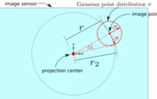
Figure 1:Image distribution;Illustrated Gaussian image distri-bution (exaggerated). As it is circular, the axes can be chosen ar-bitrarily, here perpendicular and tangential to the circle. Note that for the radial axis, only the radius and hence, the angleθchanges. For the tangential axis, the radiusrincreases tor2(again: alsoθ)
as well as the angleαon the sensor.
normal 2D distributionσof an interest point selection around the correct image point. In this paperσwill always be measured in pixel units, as this is the limiting factor for accuracy. This is a reasonable assumption as in the image domain, the ability to lo-calize a point feature only depends on the pixel sizes.
The following methods work well for equal pixel sizes as the co-variance matrix of this distribution describes a circle. This is for
automated detection as well as for manual selection of interest points, which both usually are sub-pixel accurate. In figure 1 you can recognize two different axes of the distribution. At the re-spective interest points, one is perpendicular to the circle around the center of projection and the second one is tangential. As the uniform distribution is a circle, one may choose the principal axis arbitrarily (but still orthogonal).
Given the local assumption of linearity offand the selected per-pendicular axis of the uniform distribution, at a given interest point~p, with projection radiusr, we obtain:
σθ(r) = 1
2(f(r+σ)−f(r−σ)). (5)
For smallσ, this converges to the derivation off:
σθ(r) = σdf(r) dr =σf
′(r),
(6)
hence the mapping of the perpendicular axis of the Gaussian can be approximated with equation 6.
The mapping of the second axisσ7→σt, tangential to the circle with radiusr, can also be assumed linear for smallσ. It is slightly more difficult, as it involves increasing angles in the image plane but also increasing angles due to locally increasing the radius. Letxr~ be the point~xtranslated radially, by σtimes the pixel size. Let furtherxt~ be the point~xtranslated tangentially, by the same amount.
σt = arccos(τx~r(1)−C~)·(τx~t(1)−C~)
. (7)
For many cameras, the first axis with standard deviationσθ, will produce larger errors to boundary regions, as the angular dif-ference increases for most cameras, towards the imaging sensor boundaries.
The second axis,σtwill decrease with increasing radius. This is because the angular difference of the inversef−1(θ)
decreases with increasing radius.
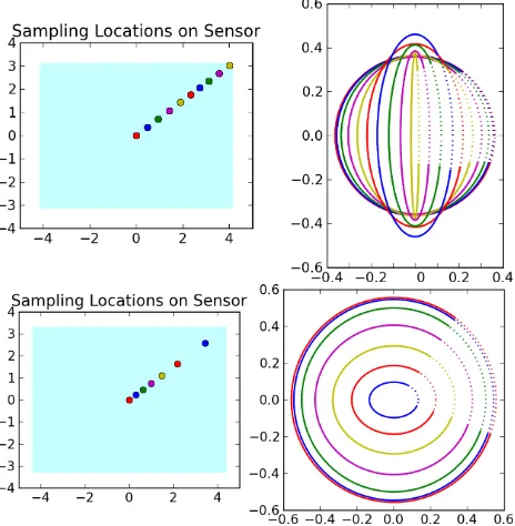
To illustrate the different effects, we created a simulation setup where the cameras are rotated such that a fixed object point cre-ates a trace on the image plane, see figure 2. In figure 3 these two different effects are plotted forσ = 0.1. Note, how the radial error (solid lines) increases for the Fisheye and the wide-angle lenses but decreases for the Catadioptric and the distortion free cameras.
The tangential error decreases with increasing radius, for all of the optical systems, roughly compensating the effect of the radial error for Fisheye and wide-angle lenses. Which of the two
ef-Figure 2: Illustration of Rotation; The rotation is applied at equidistant angle steps, such that a trace is created on the image plane, diagonal within the sensor rectangle.
fects has a greater impact depends on the camera parameters, but for our data, the overall error will usually decrease towards the boundary regions of the image sensors.
Figure 3:Influence of Radial and Tangential Error Distribu-tion;The graph shows the influence of the two axes identified in the text: radial error distribution (dotted lines) and tangen-tial error distribution (dashed lines). The solid line illustrates the overall effect, by computing the volume for the respective ellipse. σ= 0.1in pixel units. Vertical dashed lines denote maximal pos-sible sensor radius.
point error to an ellipse at 1000 mm distance. This can be found in figure 4. The Gaussian distribution with axesσθandσtcan be
Figure 4: Predicted and Measured Error Ellipses; The top graph shows the Fisheye lens, below is the Catadioptric cam-era. Error Ellipses at 1000 mm distance, predicted (dashed lines) by determining the perpendicular and tangential axis distances. Measured (solid lines) by sampling in the image plane with σ= 0.1pixel units, followed by a projection to space. The lo-cation of these samplings is illustrated in the blue area, which represents the camera sensor. Location circles on sensor are ex-aggerated for sake of visibility. All units in mm.
cast to 3D space, resulting in a cone shape with its apex at camera centerC~and its base the elliptical standard deviation.
4.3 Simulation With Real Camera Parameters
In this part of the result section some simulation results are pre-sented. These are mainly results of reconstruction with simulated noise within the image interest point locations.
4.3.1 Center Point Discontinuity As mentioned above, imag-ing of points may result in numerical instability, around image point(0,0)⊤. This can be seen for the projection and the recon-struction case, see equation 2 and 3, respectively. The simulation has shown that this concern is not confirmed, as all image points converge to zero, for input radii down to10−18. To(0,0)⊤, ex-actly. On the other hand, the inversion needs to be investigated.
Figure 5: Numerical Stability Test;When back-projected, the lower graph shows the distance to the original points around zero.
Mapping radius to a direction vector/ray involves numerically in-verting the projection model. In equation 3 a very similarǫ oc-curs. As you can see in figure 5, with our current implementation of the inverse computation off (the Python libSciPy: fsolve), there are some minor instabilities. However, these are very small, neglectable.
These experiences may lead to set the thresholds toǫ= 10−10
, for instance, to avoid division by zero in cases where object points image exactly to(0,0)⊤and vice versa.
4.3.2 Overall Error and Effect of different baselines Just like the illustration in figure 2, we rotate all the cameras such that the diagonal elements are imaged. We sample a givenσ Gaussian distribution around the currently project image point. This image point was projected from a fixed object pointX~ = (0,0,−1000)⊤. The second camera is an optimal, error free camera, moved along theX-axis with a given baseline. This al-lows for evaluation of the first camera, only. Figure 6 shows, that indeed, the smallest baseline produces the largest error, though this is not a surprise. More importantly, errors decrease with im-age points towards the imim-age sensor boundaries. This effect is a very dramatic one for the Catadioptric and the distortion free camera. Overall, this result confirms the earlier analytical predic-tion, where tangential and perpendicular errors roughly add up to the final error.
4.4 Real Image Data
The above analyses consider fixedσpositional noise, only. This gives a very nice theoretical illustration of the problem. Without changing any of the considerations, the points may have different individualσ. This theory may be applied for (manual) point de-tectors, for instance.
However, automated interest point detectors are actually slightly more region based, due to scale-space detection and neighbor-hood sampling. Probably, this results in a radius dependent posi-tioning accuracy.
Figure 6: Different Baselines; This figure illustrates the effect of different baselines on 3D reconstruction. The graph shows the simulation for aσ = 0.1pixel units. Plotted are the average reconstruction error values for each radius.
for instance. The Epipolar geometry reduces the search domain from a two dimensional space to a one-dimensional one. However, here this involves numerically inverting the projection and other difficulties such as finding the closest point on the pro-jection curve. Hence, one might as well use a different approach, which implicitly models the Epipolar constraint.
In the following, the approach is illustrated: First of all, potential matches are obtained, utilizing an approximately nearest neigh-bor search (ANN), based on feature distances. For all these po-tential matches compute the reconstruction in space and reproject to both cameras. Similar to the distance of both rays to the recon-structed point, a score can be evaluated in the image based on the given distributionσ.
Obviously, if both image points are subject to the Epipolar ge-ometry, the reprojection will map to the original points, exactly. If the Epipolar constraint is violated, the reprojection will move away from the original point. Given the original image points~x, ~
x′, the reconstructed pointX~ and the reprojected image points ~
xp,x~′p, a score can be defined as:
s(X~) = G~x,σ(xp~)·Gx~′,σ′(x~′p), (8)
whereG~x,σ is the Gaussian density withσaroundX. The nor-~ malized version of the score, here
sn(X~) = sn(X~)
G~x,σ(~x)·G~x′,σ′(x~′)
, (9)
can be used, together with a thresholdt to decide, whether a potential match fulfills Epipolar geometry. We have determined σ= 0.5andt= 0.01to obtain matches with separation of just more than 1 pixel from Epipolar geometry.
A SURF feature descriptor was used in combination with a Harris corner detector, see (Mikolajczyk and Schmid, 2004) for a thor-ough overview of interest point detectors. To obtain a high num-ber of interest point, a low threshold was used for the detection (i.e. Hessian was set to 50).
4.4.2 Evaluation Evaluating interest point detectors mainly involves evaluating the completely automated feature detection, matching and reconstruction process. Obviously there is a need for accurate ground truth data. There are different possible ap-proaches. On approach is a real scene, with depth is measured with a second sensor, i.e. a laser. A different approach is to use well known three dimensional shapes. We chose for a different approach: Simulation. The cameras are placed in the center of a
cube with side length of 2000 mm. Different textures (wood, for-est, urban, etc...) are used for different simulation iterations. The resections of automatically detected features can now be evalu-ated with perfectly known ground truth. This approach is illus-trated in figure 7.
Figure 7: Illustration of Simulation; The top left image illus-trates the camera placement. The top right image is the undis-torted camera image. The lower row contains a Fisheye image (left) and a Catadioptric image (right)
For each camera, different positions were sampled at:(0,0,0)⊤, the position to be compared to;(10,0,0)⊤, a small baseline po-sition, looking to negativeZaxis;(100,0,0)⊤, a larger baseline position looking to negativeZaxis;(500,500,−500)⊤, a wide baseline position, looking to the center of the front cube face,
(0,0,−1000)⊤.
Now different properties of the system can be evaluated: the qual-ity of matching (i.e. number of correct matches), the accuracy of reconstructed interest/feature points, the influence of the baseline length, the influence of perspective distortion and possibly influ-ence of radial distance to projection center. In table 1 and 2 some
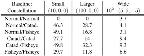
Table 1: Reconstruction Statistics for Different Camera Sys-tems: The table lists the results of reconstruction. Errors of > 100mm were considered false matches. Displayed are me-dian errors (mm), which gives a good indication of the overall performance. Numbers are accumulated over different textures.
Baseline: Constellation
Small
(10,0,0)
Larger
(100,0,0)
Wide
102·(5,5,−5)
Normal/Normal 0 0 3.7
Normal/Catad. 46.3 28.7 4.1
Normal/Fisheye 49.1 16.8 3.1
Catad./Catad. 27.7 14 9.4
Catad./Fisheye 49.8 32.3 9.3
Fisheye/Fisheye 29.7 11.8 6.6
of the answers are given. For Fisheye and Catadioptric cameras a small baseline is too small, most likely due to the compressed projection of object points at the image center. Fisheye and Cata-dioptric cameras perform similarly well. They have the least error in wide baseline situations. However, the number of matches as well as the ratio of good/bad matches is best in the medium base-line situation. This is likely due to a larger overlapping field of view and similar distortion of corresponding features in these sit-uations.
Table 2: Number of Matches for Different Camera Systems: This table lists the number of correct (error<100mm) matches vs the number of wrong matches.
Const/Base Small Larger Wide
Norm/Norm 79677/6321 84468/346 6004/4254 Norm/Catad 364/3103 2585/1211 5866/1440 Norm/Fish 3998/11387 12241/4078 8644/3131 Catad/Catad 56712/27514 61263/6147 5223/2634 Catad/Fish 1937/12889 10981/6710 7653/2858 Fish/Fish 50911/24410 59520/5775 10148/4053
error increases unexpectedly for wide baseline situations. To answer the question of radial distortion and perspective influ-ence on automatically detected features, we decided to evaluate the three homogeneous and heterogeneous camera systems. This means, at baseline distance of only 10 mm two cameras of the same type will likely not cause projective problems and follow the above mentioned theory for point features, whilst in the case of heterogeneous camera systems, the effect of different perspective distortion will arise and cause larger errors towards larger radii.
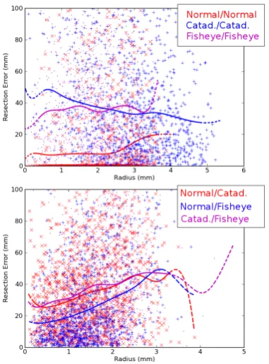
These suppositions are roughly confirmed by the results presented in figure 8. Especially for heterogeneous systems, the error in-creases towards the sensor border, mainly due to different projec-tive distortions.
For homogeneous systems, one can see the predicted decreasing effect for Catadioptric cameras. For both other systems, it is dif-ficult to recognize a specific pattern.
Figure 8:Error Evaluation of Two Camera Systems;The up-per graph shows the error plot for homogeneous systems, which reflects similar projective distortion at roughly the same radial sensor distance (small base line). Below are heterogeneous sys-tems, the maximum of both radii is used for plotting. Solid lines represent smoothed least squares fit of the data (Splines). Dashed parts are with little data. Not all of the data is plotted due to heavy cluttering of the graph.
5 CONCLUSIONS AND FUTURE WORK
This article presents accuracy analysis for stereo processing with generic camera projection models, with a main aspect on radially induced errors.
It has been shown, that for point features errors tend to decrease with larger radius from the projection center, for all types of cam-eras. Additionally, for two camera systems, the main influence for detectors like SURF is the differently distorted appearance of corresponding features. For heterogeneous camera features this means increase in reconstruction error for larger sensor radii. An-other point to mention is the general decrease in accuracy for om-nidirectional two camera systems, mainly because much more of the scene is imaged to the same image resolution.
The simulation hasn’t considered additional error sources like possible overlaps, lighting difference, point spread functions and other influences. Fixed and exact camera parameters have been assumed. But if the uncertainty parameters are known it is pos-sible to adapt the above theory by means of error propagation. Lastly, it might be useful to additionally compare different inter-est point detectors/descriptors.
ACKNOWLEDGEMENTS
Dominik Rueß and Kristian Manthey would like to acknowledge financial support of the Helmholtz Research School on Security Technologies.
REFERENCES
Brown, D., 1971. Close range camera calibration. Photogram-metric Engineering 37, pp. 855 – 866.
Fitzgibbon, A., 2001. Simultaneous linear estimation of multi-ple view geometry and lens distortion. In: Computer Vision and Pattern Recognition, 2001. CVPR 2001. Proceedings of the 2001 IEEE Computer Society Conference on, Vol. 1, pp. 125 – 132.
Hartley, R. I. and Zisserman, A., 2004. Multiple View Geometry in Computer Vision. Second edn, Cambridge University Press.
Kraus, K., 2004. Geometrische Informationen aus Photographien und Laserscanneraufnahmen. de Gruyter, Berlin.
Luber, A. and Reulke, R., 2010. A unified calibration approach for generic cameras. In: The international archives of the Pho-togrammetry, remote sensing and spatial information sciences, pp. 399 – 404.
Luber, A., Rueß, D., Manthey, K. and Reulke, R., 2012. Calibra-tion and epipolar geometry of generic heterogenous camerasys-tems. In: ISPRS World Congress Melbourne, in press.
Ma, L., Chen, Y. and L. Moore, K., 2004. Rational radial tion models of camera lenses with analytical solution for distor-tion correcdistor-tion. IJIA.
Mikolajczyk, K. and Schmid, C., 2004. Scale & affine invariant interest point detectors. International Journal of Computer Vision 60(1), pp. 63 – 86.