METHODS
A viability analysis for a bio-economic model
C. Be´ne´
a,*, L. Doyen
b, D. Gabay
baCEMARE(Centre for the Economics and Management of Aquatic Resources),Dept.of Economics,Uni6ersity of Portsmouth,
Locksway Road,Southsea Hants PO4 8JF,UK
bCNRS,Centre de Recherche Viabilite´-Controˆle,Uni6ersite´ Paris-Dauphine,Place du Mare´chal de Lattre de Tassigny,75775Paris,
Cedex16,France
Received 23 November 1998; received in revised form 11 October 2000; accepted 17 October 2000
Abstract
This paper presents a simple dynamic model dealing with the management of a marine renewable resource. But instead of studying the ecological and economic interactions in terms of equilibrium or optimal control, we pay much attention to the viability of the system or, in a symmetric way, to crisis situations. These viability/crisis situations are defined by a set of economic and biological state constraints. The analytical study focuses on the compatibility between the state constraints and the controlled dynamics. Using the mathematical concept of viability kernel, we reveal the situations and, if possible, management options to guarantee a perennial system. Going further, we define ‘overexploitation’ indicators by the time of crisis function. In particular, we point out irreversible overexploitation configurations related to the resource extinction. © 2001 Elsevier Science B.V. All rights reserved.
Keywords:Renewable resource; Fishery; Bio-economic model; Overexploitation; Viable control
www.elsevier.com/locate/ecolecon
1. Introduction
Economics of natural resources relies mainly on interactions between economic and biological (or ecological) dynamics, which makes the problem both interesting and difficult (Wilen, 1993; Vedeld, 1994; Be´ne´, 1997; Hartwick and Olewiler,
1998). Over the past decades, the topic has re-ceived growing attention because of the recent emergence of a common ‘environmental issue consciousness’ and also because natural resource exploitation has been shown to be characterized by very frequent ‘market failures’ (Tisdell, 1991; Pearce and Warford, 1993). This paper concen-trates on the example of marine renewable re-sources and their economic exploitation through fisheries.
Most economic models addressing the problem of renewable resource exploitation are built on the * Corresponding author. Tel.:+44-2392-844244; fax:+
44-2392-844037.
E-mail addresses: [email protected] (C. Be´ne´), [email protected] (L. Doyen), [email protected] (D. Gabay).
frame of a biological model. Such a model may account for the demographic structure (age or size classes) of the exploited stock (trees, fish popula-tion) or may attempt to deal with the inter-species dimension of the exploited (eco)system. However, biologists have often found it necessary to intro-duce various degrees of simplification to reintro-duce the complexity of the analysis, and one of the simplest models used in population dynamics is the ‘logistic model’. In such a model, the stock, measured through its biomass, is considered globally as one single unit without any consider-ation for the structure populconsider-ation, and its growth is materialized through the logistic equation,
x;(t)=dx
dt(t)=rx(t)
1− x(t)l
=f(x(t)),where x(t) stands for the resource biomass; l is the limit carrying capacity of the ecosystem andr
is the intrinsic growth rate of the resource. When fishing activities are included, the model becomes the Schaefer (1954) model
x;(t)=f(x(t))−h(t),
where h(t) is the harvesting flow at time t. It is frequently assumed that the catch rate h is pro-portional to both biomass and extraction effort, namely,h=qex, whereestands for the extraction effort (or fishing effort, an index related, for instance, to the number of boats involved in the activity), and q is a constant parameter usually referred as the catchability coefficient. At equi-librium, when the exploitation rate equals the population growth, one obtains the so-called sus-tainable yield associated with the fishing effort by inverting the relation
e=r
q
1−x
l
=s(x).The economic model, which is directly derived from the Schaefer model, is the Gordon model (Gordon, 1954), which integrates the economic aspects of the fishing activity through the fish price p and the fishing costs cper unit of effort. Assuming that the profit is defined by P=
pqex−ce, one can compute the efforte¯
maximiz-ing P. The Gordon model prediction, when an
open access situation occurs (i.e. when no
limita-tion is imposed on the fishery’s effort), is that the rent generated by the activity is dissipated as the effort expands beyond e¯ and the economy con-verges toward the so-called ‘open access bionomic equilibrium’.
Although it suffers from a large number of unrealistic assumptions (some of them ensuing directly from the Schaefer model limitations), the Gordon model displays a certain degree of con-cordance with empirical fisheries histories (Wilen, 1976). This is probably the reason why, along with its indisputable normative character, it has been regularly used as the underlying framework by optimal control theory since the latter has been introduced in fisheries sciences (see, for instance, Clark, 1976; Clark and Kirkwood, 1979; Goh, 1979; Charles, 1983; McKelvey, 1985; Cohen, 1987).
In optimal control theory, assuming a fixed production structure (i.e. constant capital and labor), the problem can be stated as the inter-tem-poral maximization of the profit with respect to the fishing effort e(t)
where d represents the social discount rate and
x(·) is the solution of the control system,
!
x;(t)=f(x(t))−qe(t)x(t), 05e(t)5emaxx(t)]0.
These various developments, however, did not prevent optimal control theory from suffering crit-icisms regarding its applicability to fisheries man-agement. One has observed that fishers’ decisions are seldom driven by the search for direct optimal-ity (Hilborn and Ledbetter, 1979; Bockstael and Opaluch, 1983). In order to maximize the objective function, one may also in some cases have to follow optimal solutions that bring undesirable outcomes. Two typical examples of these undesirable conse-quences are (i) negative profits: the optimal strategy requires closing the fishery for a while (which, practically, implies some fixed costs not taken into account), and (ii) resource extinction: Clark (1973) showed that it would be optimal to ‘liquidate’ the resource and to re-invest the capital in another activity when the resource growth rate is lower than the discount rate.
Optimal control theory has not only been criti-cized for the outcomes that it may bring about. It also suffers some limitations inherent in the opti-mization principle itself. On one hand, the optimal solution path is generally unique, which does not allow for possible alternate strategies. In addition, it is strongly related to the choice of the discount factor d, which is itself rather arbitrary.
All these remarks show the interest in addressing the problem from a different perspective, attempt-ing in particular to reconcile ecological and eco-nomic issues. This is the way we choose in the present paper by looking for some instantaneous and simultaneous ‘criteria’ that materialize the ‘good health’ of the bio-economic system, i.e. its viability. The viability approach (Aubin, 1991) deals with dynamic systems under state constraints (see also, Clarke et al., 1995). The aim of this method is to analyze the compatibility between the (possibly uncertain) dynamics of a system and state constraints and to determine the set of controls (or decisions) that would prevent this system from entering crisis i.e. from violating its viability con-straints. The present study is an attempt to apply this approach to the case of the management of renewable resources and especially to fisheries. We refer to Bonneuil (1994), Doyen et al. (1996) and Be´ne´ and Doyen (2000) in other contexts, and to Toth et al. (1997) for a similar framework termed the Tolerable Windows Approach. Here we define
the viability from the viewpoint of a government that aims at maintaining the fishery in a sustainable way. To achieve this, a condition (or constraint) of net benefits (positive balance sheets) of the fishing activity is imposed at any time on the resource and the effort levels. Whenever one assumes some fixed costs, it appears that this economic constraint induces a minimal threshold for the renewable resource, which is interesting if the government policy aims at reconciling ecological and economics objectives. Then, using the mathematical concept of viability kernel (Aubin, 1991), we make clear the need to anticipate the dynamics of the system to maintain its viability. This analysis allows us to identify situations of overexploitation and the adaptive regulations required to prevent deficits and/or overexploitation situations from occurring. A second mathematical concept, the time of crisis function (Doyen and Saint-Pierre, 1997), is then used to refine the overexploitation analysis. In particular, this overexploitation indicator allows us to identify two different types of crises, the re-versible crises and the irrere-versible ones. It shows how the irreversible crisis situations are linked to the resource extinction.
At this stage, we must confess that our paper does not deal with exogenous uncertainty, risk and stochasticity. We are convinced that scientific un-certainty is a basic feature to take into account for a relevant implementation of the precautionary principle. In particular, irreducible uncertainty per-taining to marine ecosystems is one important explanation of failures in the management of fisheries as Conrad et al. (1998) and Lauck et al. (1998) pointed out using a probabilistic framework. A work integrating uncertainty in a viability anal-ysis can be found in Be´ne´ et al. (1998) with the natural growth parameter of the resource fluctuat-ing in a given interval.1
But, for sake of simplicity, we restrict the present study to a deterministic control approach.
1If the probability distributions are known, then some
2. The model
2.1. The dynamics
The natural growth rate of the resource x is represented by a logistic law f depending on the intrinsic growth parameter r\0 and the limit capacityl i.e.
f(x)−rx
1−xl
.Taking into account that harvesting is propor-tional both to the biomassxand to the fishing effort
e, we consider the following dynamics for the renewable resource
x;(t)=f(x(t))−qe(t)x(t),
where q stands for the catchability coefficient. We furthermore assume that the time variation of the effort is bounded,
e;(t)=u(t), u(t)U=[u−,
u+] (1)
This assumption is a way to model the rigidity of the decision since it implies the continuity of effort with respect to time and thus rules out jumps of harvesting. For instance, it means that a decrease or an increase in number of used boats requires time to be completed. We furthermore suppose that
u−505
u+ which means that the effort can be
kept constant (case e;=0).
We obtain the following control differential system where the state variables are (x,e) and the control variable isu,
!
x; (t)=f(x(t))−qe(t)x(t),e;(t)=u(t),u−5u(t)5u+ (2)
2.2. The 6iability constraints
A second step is to express state variable con-straints from a regulating (say a government) agency viewpoint.
First, we impose an ecological constraint in the sense that the government policy requires a mini-mum level xmin\0 for the resource. Such a safe minimum biomass level (SMBL) might be identified by biologists,
xmin5x(t), Öt]0. (3)
The second constraint concerns the fishing effort
e(t). We assume that capital and labor involved in the production process remain constant; therefore,
e(t) is constrained by a fixed production capacity. We denote this limit capacity emax and we thus identify a second constraint,
05e(t)5emax, Öt]0. (4)
Furthermore, we consider that the government agency seeks to guarantee the sustainability of the activity by maintaining a global positive net benefit in the sector at any time. Let us denote byR(x(t),
e(t)) the fleet’s global balance sheet, defined as the difference between the fleet’s total income and its total production costs. Therefore, the benefit con-straint reads as follows,
R(x(t),e(t))=pqe(t)x(t)−ce(t)−C]0,
Öt]0, (5)
where p\0 represents the (exogenous) unit fish price;c\0 denotes the cost per unit of effort and
C\0 is a fixed cost, which may include, for instance, a fixed amortization of the capital stock (boats, navigation and search devises, fishing gears, …). Note first that this constraint (Eq. (5)) is more conservative than the classical enterprise’s shut-down (SD) or minimum operating condition defined in of micro-economic theory.2
2In standard micro-economic theory, an enterprise is said to
Let us also point out that the net benefit con-straint (Eq. (5)) induces the resource biomass to be strictly greater thanc/pq, namely, an ecological constraint. For sake of simplicity, we assume that,
xmin5
c pqBl.
Note also that this same constraint (Eq. (5)) yields a strictly positive minimal effort (and har-vesting) since
e(t)] C
pqx(t)−c\0.
This can be related, for instance, to an employ-ment requireemploy-ment.
Notice also that constraint (Eq. (5)) material-izes a difference between the viability approach and the optimal control approach. In the optimal control approach, the value to optimize would be the present value of net revenues
0 e
−dt
R
(x(t),e(t))dtThe optimal solution3 may require the shutdown of the activity for a while (e(t)=0), which induces a negative balance for the period and thus leads to the violation of the constraint (Eq. (5)). Furthermore, we assign an equal weight to every time period, thereby avoiding the discus-sion with respect to the choice of the discount factor.
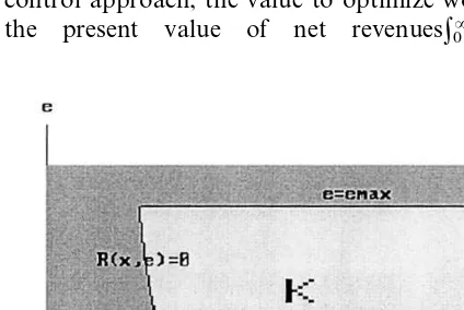
To summarize the viability constraints, we de-note by K the constraint (or target) set repre-sented in Fig. 1 and defined by
K={(x,e)R2, 05e5e max,
R(x,e)=pqex−ce−C]0}. (6)
Hereafter, we shall say that a trajectory (x(.),
e(.)) is viable in K if we have,
(x(t),e(t))K, Öt]0.
3. A viability analysis
A first question that arises now is to determine whether the evolution (Eq. (2)) is compatible with the set of constraints K defined by Eq. (6). In other words, we aim at revealing levels of resource and effort of the constraint domain K that are associated with a viable trajectory in K and thus with a viable regulation (open-loop) tu(t). To achieve this, we proceed in several steps: identifi-cation of viable stationary points, of viability niches, of the viability kernel and computation of the viable regulations associated with it. In order to restrict the mathematical content of the paper, we omit the proofs of the different results pre-sented below; these proofs can be found in Be´ne´ et al., 1998.
3.1. Viable stationary points
The first step of the analysis concerns the viable stationary points of the system, which correspond to x; =0, e;=0. Because of the constraint x(t)]
xmin\0, the solutionx=0 is clearly not a viable equilibrium. The others solutions, referred as the ‘sustainable yield levels’ in the classical approach, are defined by,
Fig. 1. In grey, the domain of viability constraintsKdelimited by the two constraints 05R(x,e) ande5emax.
of the article, we assume the government agency to be only interested in the long run viability of the sector in ensuring that condition (Eq. (5)) holds true.
3At this stage, let us emphasize that viability and optimality
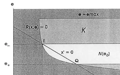
Fig. 2. The viable stationary points (segment EQ) and, in white, the viability niches.
Remark 1. The first condition in (Eq. (7)) reveals a minimum intrinsic growth rate value r* neces-sary to ensure the existence of a viable equi-librium while the second condition emphasizes the necessity of a minimum production capacity e+
induced, in particular, by the occurrence of the fixed costC. These thresholds will play an impor-tant role for the computation of the viability kernel.
3.2. Viability niches
As a second step of the analysis, we identify what we call the viability niches. These viability niches correspond to initial resource level x(0)=
x0such that the resulting evolution, with a perma-nent policy e(t)=e0, remains viable. They correspond to the most favorable situation since no regulation is needed and the effort does not have to be changed to guarantee viability. The niches N(e0) are thus defined by,
Clearly, viable equilibria are part of viability niches. As illustrated on Fig. 2, it turns out that the nichesN(e0) exist whenevere0[e+,e−] where we denote by e− the effort value,
e−=s(x−)= r
2q
1−c−D
pql
.This requires condition (Eq. (7)) to hold. In the present case, the niches are defined by,
N(e0)=
(C/e0)+cpq , +
n
.3.3. Viability kernel and o6erexploitation
The next step is to study the whole viability of the system using the concept of viability kernel. The viability kernel, denoted by Viab(K), corre-sponds to the set of all initial conditions (x0, e0)
e=s(x)=r
q
1−x
l
and u=0.These equilibria are viable whenever (x,
s(x))K. It can be shown (Be´ne´ et al., 1998, Appendix A1) that,
Proposition 3.1. A necessary and sufficient condi
-tion for the existence of 6iable equilibria for the
system (Eq. (2)) is that
Á
In that case,the set of6iable equilibria corresponds
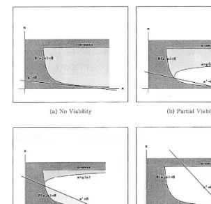
Fig. 3. Viability kernels for different values of the parameterr. In white, the viability kernel Viab(K), in grey the overexploitation zone, OZ=K¯Viab(K).
such that there exists at least one trajectory starting from (x0, e0) that stays in the set of constraints K. In other words,
Viab(K)=
!
(x0,e0)KÃ Ã Ã
×u(·) such that the solution (x(·),e(·)) of (2), starting from (x0,e0), is viable in K
"
The viability kernel differs from the niches in that, for the kernel, regulations through changes in effort can take place, thus allowing the viability to be enlarged. To focus on over-exploitation issues, we assume that,
u+] max
x\x+
g%(x)(f(x)−qg(x)x), (8)
whereg(x)=C/(pqx−c). This condition (Eq. (8)) is related to the maximal rigidity of effort and
guarantees4 the possibility to increase sufficiently the effort for high levels of resource and low levels of effort.
We can distinguish three qualitative con-figurations for the viability kernel, depending mainly on the value of the resource parameter r. These three cases are illustrated in Fig. 3.
Case 1. Global viability (Fig. 3d). The most favorable case takes place when the viability kernel equals the whole set of constraints K, i.e. Viab(K)=K. This situation occurs mainly if the intrinsic growth rateris high enough (see proof in Be´ne´ et al., 1998; Appendix A3).
4This condition makes sense since it can be checked that
Proposition 3.2.If the conditions(Eqs. (7) and (8))
hold true and if
emax5e
Remark 2. This statement means that whenever the production capacity emax is sufficiently low (still assuming that the second condition of Eq. (7) is not violated) or, in a symmetric way, whenever the resource growth rate r is high enough, viability holds everywhere and no over-exploitation occurs. In such a case, every viable situation turns out to correspond to a viability niche and the government agency does not need to regulate the fishery. In such a ‘scenario’, the maximal fleet size is too moderate to induce any dangerous mortality on the exploited resource.
Case 2(Partial6iability(Fig. 3b and c)). The most significant and interesting case occurs when the viability kernel Viab(K) is a strict and non-empty subset5
ofK. This case occurs mainly when condi-tion (Eq. (9)) does not hold true i.e. emax\e
−.
To neglect under-exploitation issues, we still assume that Eq. (8) holds. In that case, one can prove (Be´ne´ et al., 1998, Appendix A2) that the viability kernel is defined as follows.
Proposition 3.3. Under assumptions (Eqs. (7) and (8))and if emax\e−,the6iability kernel Viab(K)is
a strict and non-empty subset of K and it is defined by,
Viab(K)={(x,e)K,x]g(e) if e]e−},
where g(x) is the solution of the differential equa
-tion on[e−, e
Remark 3. The curve g, which defines the upper boundary of the viability kernel, corresponds to a trajectory satisfying e;=u− and reaching the
vi-able equilibrium point (x−, e−) (see Fig. 3b and
c). In fact, the curve grepresents the states of the system where it is necessary to change the control and thus the effort in order to prevent the system from leaving the domain of constraintK. In other words, this is the ‘last’ zone and consequently the ‘last’ moment where it is still possible to change the extraction effort in order to preserve economic viability. The existence of this boundary thus makes clear the need to regulate the fishery and to anticipate the dynamics of the system in order to avoid a crisis (here a failure to cover costs). In particular, it emphasizes the need to reduce as drastically as possible the effort ewith respect to the capital rigidity (Eq. (1)) when attaining this curve. Note that part of this curve g (especially the portion around the equilibrium point (x−, e−)) is located in a zone characterized by a ‘low’
resource and a ‘high’ effort levels. This is quite coherent with general expectations since many of the problems encountered in renewable resource management relate to the combination, low re-source level – high extraction rate.
Along with this, we can identify the over-ex-ploitation zone denoted by OZ as the set
OZ=K¯Viab(K)={xK, xQViab(K)}.
This set OZ (in grey in Fig. 3)materializes the situations where the extraction effort is too high and would drive the system to a crisis (through a decrease of the resource and then a net revenue crisis) despite admissible regulations having been applied.
Case 3.No viability (Fig. 3a). It turns out that the viability kernel is empty whenever condition (Eq. (7)) related to the existence of a viable equilibrium is not satisfied. Indeed, an equilibrium located in
K is always a state of the viability kernel.
Proposition 3.4. If condition (Eq. (7)) is not sa
-tisfied, then Viab(K)=¥.
Remark 4. In particular, this means that, if the intrinsic growth rate value r is smaller than the thresholdr* defined in Eq. (7), then the system is not sustainable; in other words, we face an over-exploitation situation in every case, i.e. OZ=K.
3.4. Viable regulations: how to a6oid
o6er-exploitation
The viability kernel revealed the states biomass-effort compatible with the constraints. The present step is to compute the viable management options (decision or control) associated with it. For this purpose, we introduce the viable regula-tion map U(x, e) which represents the controls
u=e; that can maintain viability for a state (x,e). For any point (x, e) in the viability kernel Vi-ab(K), we know that this regulation set is not empty. We consider the case of partial viability, namely,
Viab(K)={(x,e)K, x]g(e) if e]e−}.
Under the assumptions (Eqs. (7) and (8)), we can prove (Be´ne´ et al., 1998, Appendix A4) that
U(x, e) is then defined by,
Remark 5.From the calculation of this regulation map U, it appears that the only mandatory unique regulation occurs when the anticipation of a revenue crisis is required, i.e. whenx=g(e). In that case, the choice inU(x,e) reduces tou−.For any other situations within the viability kernel, several viable regulations and viable policies are possible. This means that policy-makers are of-fered different viable alternatives, which extends their flexibility with respect to the multiple,
evolv-ing (or sometimes conflictevolv-ing) objectives they at-tempt to achieve. This result may represent an improvement with respect to other approaches where only one solution is usually proposed.
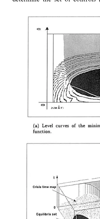
4. Time of crisis and irreversibility
In this section, we go a step further in the analysis of the system viability by using the con-cept of time of crisis (Doyen and Saint-Pierre, 1997). We have pointed out above the possible existence of an ‘overexploitation’ area OZ where the dynamics lead the system to leave the domain of constraints, and in particular to violate the benefit constraint. Negative profits happen in lots of fisheries (at least for some finite period) every-where in the world. Indeed it is not unusual that fishermen have to face periods where the value of the catch does not cover the total operating costs. However, as we mentioned previously in Section 2.2, these negative cash-flows do not necessarily induce the definitive shutdown of the activity provided that they do not last for too long. Consequently, it is relevant to determine what would happen in this situation, to evaluate the corresponding level of overexploitation and, in particular, to study its irreversibility feature. So, for a given trajectory (x(.),e(.)), we measure6the straints consisting simply of the ecological mini-mal threshold (SMBL) and the maximini-mal effort capacity as follows
6The measure is taken in the sense of
H={(x,e)R2,
xmin5x, 05e5emax}.
The crisis function V provides an indicator of overexploitation and shows that three qualitative areas can be distinguished,
no overexploitation: V(x, e)=0. Inside the viability kernel Viab(K), the value V(x, e) equals 0. This emphasizes again the existence of a viable control and a solution that does not violate the state constraints K. This case has already been fully discussed above;
reversible overexploitation: 0BV(x, e)B+
. The overexploitation crisis (x, e)OZ=
K¯Viab(K) can be solved in finite time. As illustrated in Fig. 4, the cash flow crisis (RB
0) can be long, and there is a period of time during which, even with a drastic reduction of the activity (e;=u−), the resource level will
continue to decrease until it reaches a level where it can be rebuilt. In that case, the strategy is then to let the resource grow thanks to a ‘weak’ effort in order to return into the viability kernel;
irreversible overexploitation: V(x, e)= +. The crisis (RB0) induced by the overex-ploitation becomes an irreversible crisis since it leads to the ‘extinction’ (xBxmin) of the resource and therefore, to the definitive shut-down of the economic activity. From Fig. 4, it appears that this situation may happen if the effort level is set high. But it can also happen in moderate harvesting effort situa-tions when the change in strategy is decided too late, i.e. when the net revenue R(x, e) becomes negative. This can occur, for in-stance, if fishermen’s behavior is completely rigid and the reduction of effort is not ap-plied (u=0) until the viability condition (to be in K) is directly jeopardized. In that case, if the initial conditions are located above the viability curve g, the resource decreases until the trajectory reaches a point (xˆ, e0) where the viability is at stake (R(xˆ, e0)=0). If V(xˆ,
e0)= +, then, whatever the later change of strategy and regulation, the resource and thus the economic activity will collapse.
5. Conclusion
In this study, we have addressed the problem of the management of natural resource exploitation systems. We re-visit the classical dynamic fishery model within a new framework based on the concept of viability. The main purpose of this new approach is not to maximize an objective func-tion, but to analyze the compatibility between the dynamics of a system and its constraints and to determine the set of controls (or decisions) that
prevent the system from violating these viability constraints.
In the present case of a fishery model, manage-ment options are identified, assuming a determin-istic dynamics (no uncertainty) and a net benefit constraint with fixed cost. This ability to cover costs induces effort and biomass minimal thresholds and thus aims at reconciling ecological and economics requirements. The viability kernel analysis highlights the need to anticipate the sys-tem dynamics to prevent sector deficits that are related to overexploitation issues. Then, using the time of crisis concept, we evaluate different types of overexploitation. In particular, we distinguish a reversible overexploitation zone, where the system can recover from crisis and come back into the viable domain in finite time, and an irreversible overexploitation situation, which leads to the ex-tinction of the resource and to the definitive shut-down of the activity.
It is clear that the model adopted in this study is quite stylized and built on simplistic assump-tions. Future research is needed to relax some of these assumptions. In particular, we aim at in-cluding uncertainties as a basic feature for a rele-vant implementation of the precautionary principle. Capital dynamics through investment, price dynamics and market demand should also make the model more realistic. We also hope to incorporate and analyze behavior mechanisms such as cooperation with respect to the resource access issue. More generally, we believe that the viability approach may provide an interesting an-alytical framework to address some of the issues encountered in natural resource management and sustainable development.
References
Aubin, J.P., 1991. Viability Theory. Birkha¨user, Springer. Be´ne´, C., 1997. Dynamics and adaptation of a fishery system
to ecological and economic perturbations: analysis and dynamic modeling, the French Guyana shrimp fishery case. Ph.D. Dissertation, University of Paris VI, Paris, p. 236 (in French).
Be´ne´, C., Doyen, L., 2000. Storage and viability of a fishery with resource and market dephased seasonalities. J.
Envi-ron. Resour. Econ. 15, 1 – 26.
Be´ne´, C., Doyen, L., Gabay, D., 1998. A Viability Analysis for a Bio-economic model. Cahiers du Centre de Recherche Viabilite´-Jeux-Controˆle, N 9815.
Bockstael, N.E., Opaluch, J., 1983. Discrete modeling of be-havioral response under uncertainty: the case of the fishery. J. Environ. Econ. Manage. 10, 125 – 137.
Bonneuil, N., 1994. Capital accumulation, inertia of consump-tion and norms of reproducconsump-tion. J. Populaconsump-tion Econ. 7, 49 – 62.
Charles, A.T., 1983. Optimal fisheries investment under uncer-tainty. Can. J. Fish. Aquat. Sci. 40, 2080 – 2091.
Charles, A.T., 1989. Bio-socio-economic fishery models: labor dynamics and multi-objective management. Can. J. Fish. Aquat. Sci. 46, 1313 – 1322.
Clark, C.W., 1973. The economics of overexploitation. Science 181, 630 – 634.
Clark, C.W., 1976. Mathematical Bio-economics: the Optimal Management of Renewable Resource. Wiley, New York. Clark, C.W., Munro, G.R., 1975. The economics of fishing
and modern capital theory: a simplified approach. J. Envi-ron. Econ. Manage. 2, 92 – 106.
Clark, C.W., Kirkwood, G.P., 1979. Bioeconomic model of the Gulf of Carpentaria prawn fishery. J. Fish. Res. Board Can. 36, 1303 – 1312.
Clark, C.W., Kirkwood, G.P., 1986. On uncertain renewable resource stocks: optimal harvest policies and the value of stock surveys. J. Environ. Econ. Manage. 13, 235 – 244. Clarke, F.H., Ledyaev, Y.S., Stern, R.J., Wolenski, P.R., 1995.
Qualitative properties of trajectories of control systems: a survey. J. Dynam. Control Syst. 1, 1 – 48.
Cohen, Y., 1987. A review of harvest theory and applications of optimal control theory in fisheries management. Can. J. Fish. Aquat. Sci. 44 (Suppl. 2), 75 – 83.
Conrad, J.M., Lopez, A., Bjorndal, T., 1998. Fishery Manage-ment: the Consequences of Honest Mistakes in a Stochas-tic Environment. Working Paper in Environmental and Resource Economics, Cornell University, WP 98-11. Diaz-de-Leon, A., Seijo, J.C., 1992. A multi-criteria non-linear
optimization model for the control and management of a tropical fishery. Mar. Resour. Econ. 7, 23 – 40.
Doyen, L., Saint-Pierre, P., 1997. Scale of viability and mini-mal time of crisis. J. Set-Valued Anal. 5, 227 – 246. Doyen, L., Gabay, D., Hourcade, J.C., 1996. Risque
clima-tique, technologie et viabilite´. Actes des Journe´es du Pro-gramme Environnement Vie et Socie´te´s, CNRS, Session B, pp. 129 – 134.
Goh, B.S., 1979. The usefulness of optimal control theory to biological problem. In: Halfon, E. (Ed.), Theoretical Sys-tems Ecology; Advances and Case Studies. Academic Press, New York, pp. 385 – 399.
Gordon, H.S., 1954. The economic theory of a common property resource: the fishery. J. Pol. Econ. 82, 124 – 142. Hartwick, J.M., Olewiler, N.D., 1998. The Economics of
Healey, M.C., 1984. Multi-attribute analysis and the concept of optimal yield. Can. J. Fish. Aquat. Sci. 41, 1393 – 1406. Hilborn, R., Ledbetter, M., 1979. Analysis of the British Columbia salmon purse-seine fleet: dynamics of movement. J. Res. Board Can. 36, 384 – 391.
Lauck, T., Clark, C.W., Mangel, M., Munro, G.R., 1998. Implementing the precautionary principle in fisheries man-agement through marine reserves. Ecol. App. 81, S72 – S78 Special Issue.
McKelvey, R., 1985. Decentralized regulation of a common property renewable resource industry with irreversible in-vestment. J. Environ. Econ. Manage. 12, 287 – 307. Pearce, D.W., Warford, J., 1993. World without End. World
Bank, Oxford University Press, p. 440.
Schaefer, M.B., 1954. Some aspects of the dynamics of popu-lations. Bull. Int. Am. Trop. Tuna Comm. 1, 26 – 56. Tisdell, C.A., 1991. Economics of Environmental
Conserva-tion. Elsevier, Amsterdam, p. 233.
Toth, F.L., Bruckner, Th., Fussel, H.-M., Leimbach, M., Petschell-Held, G., Schellnhuber, H.J., 1997. The tolerable windows approach to integrated assessments. Proceedings of the IPCC Asia-Pacific Workshop on Integrated Assess-ment Models, Tokyo, Japan, 10 – 12 March, p. 19. Varian, H.R., 1992. Microeconomic Analysis, third ed.
Nor-ton, New York.
Vedeld, P.O., 1994. The environment and interdisciplinarity. Ecol. Econ. 1 (10), 1 – 13.
Wilen, J.E., 1976. Common property resources and the dy-namics of over-exploitation: the case of the North Pacific fur seal. Research Paper No. 3, Department of Economics, University of British Columbia, Vancouver, Canada. Wilen, J.E., 1993. Bioeconomics of renewable resource use. In:
Kneese, A.V., Sweeney, J.L. (Eds.), Handbook of Natural Resource and Energy Economics, vol. I. Elsevier, Amster-dam, pp. 61 – 121 Part 1.