Ecological Economics 36 (2001) 87 – 108
ANALYSIS
Experimenting with multi-attribute utility survey methods in
a multi-dimensional valuation problem
Clifford Russell
a,*, Virginia Dale
b, Junsoo Lee
c, Molly Hadley Jensen
a,
Michael Kane
d, Robin Gregory
eaVanderbilt Institute for Public Policy Studies,1207 18th A6enue South,Nash6ille,TN37212,USA bEn6ironmental Sciences Di6ision,Oak Ridge National Laboratory,P.O.Box2008,Oak Ridge,TN37831-6036,USA
cDepartment of Economics,P.O.Box161400,Uni6ersity of Central Florida,Orlando,FL32816-1400,USA dDepartment of Ecology and E6olutionary Biology,Uni6ersity of Tennessee,Knox6ille,TN37996-1410,USA
eDecision Research,1124West19th Street,No.Vancou6er,B.C.,Canada Received 24 May 1999; received in revised form 22 May 2000; accepted 1 June 2000
Abstract
The use of willingness-to-pay (WTP) survey techniques based on multi-attribute utility (MAU) approaches has been recommended by some authors as a way to deal simultaneously with two difficulties that increasingly plague environmental valuation. The first of these is that, as valuation exercises come to involve less familiar and more subtle environmental effects, such as ecosystem management, lay respondents are less likely to have any idea, in advance, of the value they would attach to a described result. The second is that valuation questions may increasingly be about multi-dimensional effects (e.g. changes in ecosystem function) as opposed for example to changes in visibility from a given point. MAU has been asserted to allow the asking of simpler questions, even in the context of difficult subjects. And it is, as the name suggests, inherently multi-dimensional. This paper asks whether MAU techniques can be shown to ‘make a difference’ in the context of questions about preferences over, and valuation of differences between, alternative descriptions of a forest ecosystem. Making a difference is defined in terms of internal consistency of answers to preference and WTP questions involving three 5-attribute forest descriptions. The method involves first asking MAU-structured questions attribute-by-attribute. The responses to these questions allow researchers toinfer
each respondent’s preferences and WTP. Second, the same respondents are asked directly about their preferences and WTPs. The answer to the making-a-difference question, based largely on comparing the inferred and stated results,
www.elsevier.com/locate/ecolecon
Based on research supported by EPA GrantcR824699. Neither the results nor their interpretations as reported in this paper have been reviewed or endorsed by USEPA. The senior author would like to thank participants in seminars at the University of East Anglia, the Norwegian Agricultural University, the Swedish Agricultural Universities at Uppsala and Umea˚, AKF in Copenhagen, and the Beijer Institute of the Royal Swedish Academy of Sciences for helpful comments and suggestions. We are also grateful for comments on an earlier draft by Nick Hanley and Eirik Romstad.
* Corresponding author. Fax: +1-615-3228081. E-mail address:[email protected] (C. Russell).
is not straightforward. Overall, the inferred results are good ‘predictors’ of what is stated. But the agreement is by no means perfect. And the individual differences are not explainable by the socio-economic characteristics of the individuals. Since the technique involves creating a long, somewhat tedious, and even apparently confusing series of tasks (though each task may itself be simple), it is by no means clear that the prescription, ‘use MAU techniques’, holds the same level of practical as of theoretical promise. © 2001 Elsevier Science B.V. All rights reserved.
Keywords:Ecosystem valuation; Multi-attribute utility; Willingness to pay surveys; Forest attributes
1. Introduction
The literature dealing with direct methods of environmental damage or benefit estimation is large, complex, fascinating, and growing at a prodigious rate. The central concern for perhaps 90% of that literature is how seriously to take the answers that respondents give to varieties of
will-ingness-to-pay (or to accept) (WTP/WTA)
ques-tions. One version of that concern is the traditional economics worry — that people will figure out how their possible answers might affect their future welfare and conceal their true prefer-ences (reveal false ones), either free-riding or over-bidding as the situation seems to make desirable (e.g. Mitchell and Carson, 1989, ch. 6 and 7). A second version, broadly stated, is that, so far from understanding how to conceal true preferences to reap greater potential rewards, lay respondents to environmental valuation questions do not know what their preferences are and cannot possibly predict what they would be in a real as opposed to the hypothetical survey choice situation. We may think of this as the psychologists’ concern (e.g. Fischhoff, 1991; Schkade and Payne, 1994). Bohm (1994), takes a position that might be seen as a blend of the two simplified ones set out above. He stresses the hypothetical structure of the questions and the resulting unreliability of the answers. But his evidence points to a tendency to overstate WTP.
Sharpening this latter concern is the trend in the field of direct valuation toward taking on more subtle, complex, and long-term problems, such as those dealing with ecological systems,
their condition, management, and future
prospects. These extensions mean that the situa-tions being sketched and the preference and valu-ation decisions being sought are becoming more
distant from lay experience. At the same time, the information that must be transferred to the re-spondent is becoming more extensive and more complicated. In particular, questions often involve more than one environmental dimension, as con-trasted with, for example, visibility changes for which the policy effect is naturally captured by a scalar.
The work reported on here was motivated by the cognitive concern. It picks up the suggestion made by Gregory et al. (1993) (also Gregory and Slovic, 1997) that multi-attribute-utility theory (MAUT or just MAU) can provide the
founda-tion for an alternative approach to valuafounda-tion.1
They make the case that MAU, in principle, addresses both the multi-dimensionality and the unfamiliarity of the new valuation challenges by providing a set of cognitively simpler tasks. Our goal was to test the proposition that the use of MAU Survey techniques will make an identifiable and useful difference in results obtained from respondents to a survey instrument dealing with a multi-dimensional environmental ‘good’. Other researchers have made a similar point in the con-text of using multi-criteria decision-making meth-ods (MCDM) as a means to quantify stakeholder values in complex economic or environmental risk problems where prior experience is limited (e.g. Hobbs and Horn, 1997).
C.Russell et al./Ecological Economics36 (2001) 87 – 108 89
The remainder of the paper is divided into five sections. Section 2 describes the setting, the choice of attributes, the survey instrument and method of its application, and summarizes the characteris-tics of the respondent samples. Section 3 contains the results from the full MAU survey, including: most- and least-preferred levels of the attributes and their ranks and weights; stated WTP for the availability of the most- rather than least-pre-ferred level of the respondent’s most important attribute; and the implications of these responses for the respondent’s preferences over and WTP for differences between the blended forests.
In Section 4 the tests and their results are described: evidence of confusion when respon-dents directly confront the multi-dimensional comparisons of the blended forests; and matches between implied and stated preferences over and WTP for differences between those forests. Efforts to explain the respondent-by-respondent results for these matches are also reported. Section 5 takes up the possibility that the results reflected the educational effect of completing the full MAU questionnaire. Results are reported in terms of extent of apparent confusion (intransitive prefer-ence statements) and comparisons of stated
pref-erences and WTP amounts with the
corresponding responses of the ‘educated’ sample. Section 6 includes our interpretation of the results and suggestions for further work.
2. Setting, attributes, and sample
2.1. The setting and the attributes
The setting we chose for this test is a Southern
Appalachian forest ecosystem.2 We have
else-where (Russell et al., 1997) discussed the
develop-ment of the attributes, how they were described in words and given visual form, and how the setting was simplified. Briefly, however, we required the attributes to satisfy (as closely as possible) five conditions:
1. Because the questions asked involve having the respondent imagine changing each at-tribute independently, they should be orthogo-nal, or as close to that condition as feasible, given the other requirements.
2. The number of attributes should be small — certainly smaller than the 18 ecological indica-tors used in the Environmental Monitoring and Assessment Program (EMAP) as descrip-tors of forests (Lewis and Conkling, 1994). Our goal was to stay below eight as suggested by some of the literature on the difficulties people have with multidimensional judgments (e.g. Miller, 1956; Phelps and Shanteau, 1978). (A key part of our test described later involves such a judgment.)
3. The attributes should be describable by combi-nations of simple words and straightforward
visual images (photographs, schematics,
cartoons).
4. The attributes should be ecologically meaning-ful (i.e. interpretable by ecologists as providing a summary description of the forest). Several individual measurements might be summarized
in one or more index-like measures.3
5. The attributes should relate to people’s rea-sons for valuing forests as well as to scientific concerns.
The last two of these requirements for at-tributes interact in an interesting way. One might
imagine trying to satisfy the last (c5) by
includ-ing a ‘forest quality ladder’, akin to the ‘water quality ladder’ developed at Resources for the Future for a contingent valuation study of the benefits of water pollution control. This ladder showed supportable recreation uses of water
bod-2This choice was originally made because we were, at the time of writing the proposal, working on an EPA/EMAP project involving linking Environmental Monitoring and Assessment Program (EMAP) ecological indicators for a forest system to societal values. We had anticipated that the EMAP project would give us a substantial head start in devising the attribute set for this study. In the event, however, the project was canceled by EPA before we had obtained the anticipated results, though we had gathered focus group input on how lay people think about forests and what they value in and about them.
ies changing as water quality — proxied by dis-solved oxygen — increased (Mitchell and Carson, 1984). The analog would have been to attach the sources of human values for forests to an index of forest ‘quality’ for those uses, thus making the forest valuation problem unidimensional. The key to the modest success of this approach in the water quality arena, however, was the plausibility of choosing dissolved oxygen as the single under-lying measurement.
But in forests, there is no simple array of ‘functions’ (sources of values) related to any single underlying attribute or measurement determining the suitability of a particular piece of forest for providing all or even many of those services. And, given a multidimensional description of a particu-lar forest, it is possible, even likely, that different individuals will judge that forest differently in the matter of how well it would serve a particular function, such as recreation service provision. Said the other way round: describing a forest as ‘good for activity A’ would, in general, call up ecologically different forests in the imaginations of different respondents. Thus, it seemed (and seems) to us dangerous to substitute functions for ecological descriptors, while still claiming to be faithful to ecological consistency. That is, the
straightforward approach to satisfying c5 (and,
in the process, reducing the problem to a single
dimension) promised to violate c4.
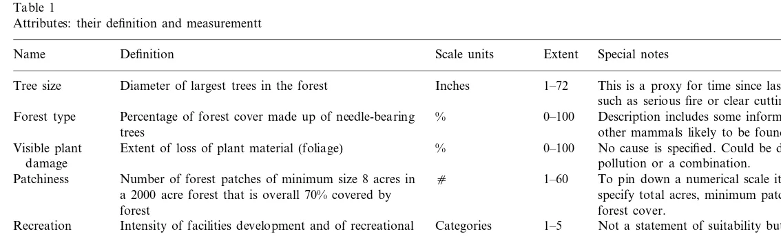
The six attributes we used, along with their scales and special notes on visual presentation, are summarized in Table 1. All descriptions consisted of combinations of words and pictures. Schemat-ics were used to help people picture ‘patchiness’.
The reader will note that nothing is said about
water features of the landscape/ecosystem. We
told respondents to imagine any water features they wanted, but to hold them constant across the question situations. We did not want to risk hav-ing our choice of water features distort the per-ceptions of respondents, for we knew from the literature on landscape perception that water fea-tures tend to be dominant (e.g. Coss and Moore, 1990; also Hanley and Ruffell, 1993). Similarly for topography, though we suggested they imagine the steep, rolling hills typical of much of the region (Kaplan and Kaplan, 1989). We also asked
respondents to ‘think summer’. Finally, and fur-ther to simplify, we asked respondents to assume that the conditions were to be maintained con-stant over many years. We realize that this is not ecologically realistic, but we feared making the problem more complex by trying to describe the different paths of forest change that might arise from a given current condition.
2.2. The instrument
The MAU technique involves finding attribute-by-attribute functions that relate WTP to the level of the attribute ‘provided’. For economy of pre-sentation we refer to these as ‘sub-WTP’ func-tions. Added together, they imply a total WTP for any combination of the attributes. For each re-spondent and each sub-WTP function the baseline is that respondent’s least preferred level of the attribute. This, in turn, implies that differences between alternative forests can be valued, but not a forest as opposed to no forest.
Gregory et al. (1993) give some guidance about the choice of attributes, but do not provide even the beginning of a cookbook for structuring the questions necessary to capture these functions. And while there is a huge literature on applying MAU in decisions (e.g. Keeney and Raiffa, 1976; Edwards, 1977; Merkhofer and Keeney, 1987; von Winterfeldt, 1987; Keeney, 1992), much of the work on elicitation of MAU-related judgments has involved sophisticated decision makers oper-ating in their areas of expertise (e.g. Jenni et al., 1994). Our setting is different in two very impor-tant ways: we were interested in the views of lay, not expert, respondents; and, we could expect that only a handful of respondents would know much about forests when we first encountered them. This would be true even though a substantial fraction might actually be users of forests for sightseeing, hiking, and even camping.
Vander-C
.
Russell
et
al
.
/
Ecological
Economics
36
(2001)
87
–
108
91
Table 1
Attributes: their definition and measurementt
Special notes
Name Definition Scale units Extent
This is a proxy for time since last extensive disturbance Tree size Diameter of largest trees in the forest Inches 1–72
such as serious fire or clear cutting.
Description includes some information about birds and 0–100
% Forest type Percentage of forest cover made up of needle-bearing
trees other mammals likely to be found in the forest.
No cause is specified. Could be disease, insects, Extent of loss of plant material (foliage) % 0–100
Visible plant
damage pollution or a combination.
To pin down a numerical scale it is necessary to Patchiness Number of forest patches of minimum size 8 acres in c 1–60
specify total acres, minimum patch size and total % a 2000 acre forest that is overall 70% covered by
forest forest cover.
1–5 Not a statement of suitability but of actual conditions. Categories
Intensity of facilities development and of recreational Recreation
intensity use (1=lowest level) From essential wilderness to highly developed and
intensively used.
Also a statement of actual conditions. From essentially Intensity of extractive use
Extractive Categories 1–5
zero extraction to mining or extensive logging.
bilt Institute for Public Policy Studies (VIPPS), almost all under the direction of Molly Hadley Jensen. In all we held nine focus groups over the months from May to October 1996. A total of 33 people participated in these. We also conducted seven think-aloud interviews using the entire in-strument as it then existed. These were held in the months of August through October as the instru-ment neared what we guessed would be its final form. We tried hard to bring in a wide range of ages, education levels, and (presumed) back-grounds with respect to forest-oriented activities. The earliest groups helped us settle on useful visual images and meaningful scales for the inten-sity variables. Later groups focused on structure and wording. The message of these latter groups was consistent: simplify, simplify, simplify. We tried very hard to respond, though we realize that even after about a dozen redraftings, we still probably had residual problems with jargon and technical language, too many words, too long sentences, and too complex instructions.
The tasks asked of respondents were as follows:4
1. Each respondent identified her/his most- and
least-preferred levels for each of the six forest attributes. This was done while the attributes were being explained and the relevant visuals displayed.
2. Each respondent put the attributes in decreas-ing order of subjective importance. This rank-ing was triggered by the question: ‘If you were visiting a forest in which every attribute was at your least preferred level, which one of the attributes would you change first to your most preferred level, if you could?’ This same ques-tion form was used to find the second ranked, third ranked, and so on.
3. Each respondent supplied weights for the or-dered attributes, beginning with an arbitrary
100 for her/his most important. It was stressed
that these did not have to add up to any particular number but could equally well be 100, 98, 96, . . ., 90 and 100, 10, 9, . . ., 6 or
any other decreasing but non-negative
pattern.5
4. We asked people to complete two exercises that bring in the notion of WTP for changes in the levels of individual attributes. The first exercise asked about annual WTP to help in-sure that the respondent’s most important
at-tribute would be maintained at his/her most
preferred (rather than least preferred) level in a forest of about 20 000 acres (if a square, about 5.5 miles on a side) within 1.5 h of their city, Nashville. The second asked the same question about the second most important attribute for each respondent.
The specificity about the park did not extend to name or location. The idea was just to create a context far enough from the city that it would not have to be crowded and intensively used, but close enough that it could be visited for day trips. The size is arbitrary but is intended to create a sense of scale well larger than familiar local forested parks. (It is 10 times the size of one such park used elsewhere in the instrument to remind people of the region’s topography.)
Finally, it is worth noting that arriving at this format for the question connecting attributes to WTP was a painful process. (It is described in Russell et al., 1997.) Suffice it to say here, MAU practitioners are likely to find it less than satisfac-tory. They would prefer to see a more ‘natural’ connection via another attribute linked itself to money.
Examples discussed and rejected in creating the questionnaire used here were forest industry wages and profits in the region. In our judgment the available alternatives were either just as ‘artifi-cial’ as the approach used here or would have violated the attribute independence requirement. The latter, for example, is true of the examples cited above, for the respondent could hardly be
5An extensive literature exists discussing alternative meth-ods for eliciting weights and warning how difficult it can be to achieve consistency. The methods include pairwise compari-sons and subsequent hierarchical re-composition as part of an Analytic Hierarchy Process (e.g. Saaty, 1983) or variations on the swing-weighting, lottery, or pricing-out procedures typi-cally used by decision analysts (e.g. von Winterfeldt and Edwards, 1986).
C.Russell et al./Ecological Economics36 (2001) 87 – 108 93 Table 2
The ‘blended’ forest descriptionss
Attribute First forest Second forest Third forest
25%%diameter
(1) Tree size 25%%diameter 25%%diameter
(2) Forest type 0% needle-bearing 0% needle-bearing 50% needle bearing 10% loss vegetation 30% loss vegetation (3) Visible plant damage 30% loss vegetation
5 patches
1 patch 5 patches
(4) Patchiness
3 4
(5) Recreation intensity 2
3 3
4 (6) Extraction intensity
expected to believe that forest industry profits or wages could rise in the absence of an increase in extractive activity. The former would be true of an ‘attribute’ that was the cost of an admission ticket or other version of a fee for use.
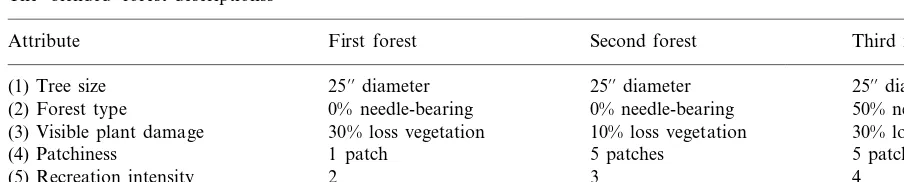
2.3. Testing for ‘a difference’
In brief, our approach to testing whether MAU ‘makes an identifiable difference’ involved creat-ing what we call ‘blended’ forests, uscreat-ing varycreat-ing combinations of five of the six attributes. These are described in Table 2. Respondents were first asked the MAU questions listed above that al-lowed us to infer the value they would put on any such forest. Then they were asked directly about their ordinal preferences over and WTP for differ-ences between three ‘blended’ forests. (The forests were labeled ‘first’, ‘second’, and ‘third’.) At the simplest level, we asked three preference ques-tions, one for each of the possible pairings of the blends. This approach gave respondents enough scope to give answers implying cyclic (intransitive) preferences. A straightforward result would then be to find a substantial number of intransitive responses, implying that people had trouble with the direct multi-dimensional comparisons. The WTP question asked, specifically, for first and second and for second and third, ‘How much would you be willing to pay annually to be able to visit regularly your preferred forest [of the pair] as opposed to the other forest’.
More complex, and more difficult to interpret, were the comparisons of:
stated and implied preference patterns
stated and implied WTPs for the differences
between the blended forests.
Again, the most straightforward outcomes would be to find very little agreement. Then, while we would have no way of saying which is ‘cor-rect’, we would at least know that there was a difference between the MAU and the more di-rectly obtained results. Because in later results, second forest turns out to be preferred to the other two by a majority of respondents, it is worth pointing out that when we ‘designed’ the blended forests, we had only informal focus group information about which attributes were likely to be most important and which levels of the at-tributes most and least preferred. We strove to produce three descriptions that would be different enough to be distinguishable, but not so different as to make the ranking questions asked about them trivially easy. The last two pages of the instrument asked basic socio-economic questions and also sought information about experience with forests, such as camping, gathering herbs, biking, and picnicking. The experience
informa-tion was used in dummy variable (did/did not)
form in subsequent regression analysis.
3. Data gathering and the respondent sample
blended forest questions, was sufficiently daunting that trying to use it as a mail survey would likely bring serious non-response problems. But neither was there money in the budget to allow us to contract for more than a handful of individual interviews. And, of course, the heavy need for visuals made telephone surveys impossible. Faced with this dilemma, we adopted a data-gathering approach based on ‘deliberative polling’ (Fishkin, 1995). That is, we convened large groups (roughly 75 people) in a conference room at VIPPS and
worked through the survey with them.6
The visu-als were made available to the entire group
simul-taneously and at low cost by using a
computerized bank of TV monitors available in
the room.7 These sessions took a bit over two
hours, a fact that made it difficult to schedule them in the evenings, which in turn interfered with sampling from the working population.
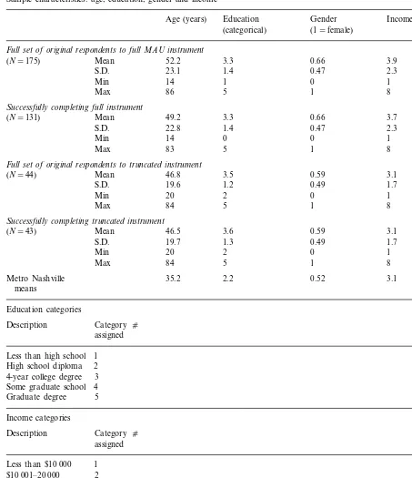
The groups assembled did cover a wide range of ages, income and educational levels. The four basic socio-economic characteristics requested from respondents were age (years), education,
gender (1=female), and income. Characteristics
of the original 175 and of those successfully com-pleting the questionnaire are described in Table 3. We refer to an exercise involving only an intro-duction to the attributes followed directly by the blended forest questions as the ‘truncated survey’ and show the characteristics of those starting and completing this exercise separately.
The message of this table is clear. Though we gathered diverse groups for our deliberative polling exercises, those groups could not be called representative of the community. In particular, they were older, better educated, better off eco-nomically, and contained more women. There is
hardly any difference between the full groups that sat down to take either survey and the corre-sponding sub-groups that successfully finished. There is, on the other hand, a somewhat better match between the smaller group that saw the truncated questionnaire and the Nashville popula-tion than between the full MAU sample and that population. But the differences between the two groups who successfully finished the surveys (131 and 43) are not statistically significant (except that the gender composition is significant at the 10% level).
There is nothing particularly striking in the data from the self-reports of forest use, and we do not show a summary here. Driving, hiking and picnicking are commonly engaged in. At the other extreme, ATV use, herb gathering, hunting, and cutting wood (as an occupation) are quite rare. The two sample groups have similar patterns of reported experience, and these experiences have been concentrated in the Southeastern US.
Note that 75% of the people who began the full survey exercise finished. Most of the ‘failures’ (26 of 44) occurred in the questions involving at-tribute preferences. Ten more people could not or did not answer the WTP question about their most important attribute. Six could not or did not answer the blended forest comparisons. One did not complete the personal characteristics section. And, finally, one person who completed all parts of the questionnaire was an outlier in WTP state-ments by more than an order of magnitude. Only one person failed to successfully complete the truncated survey.
4. Results from the surveys
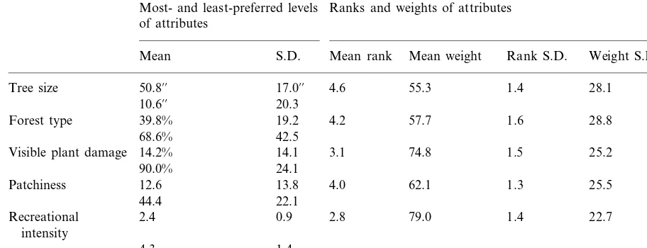
4.1. Most-and least-preferred le6els; ranks and weights
The results from the questions about most- and least-preferred levels of the attributes and the
ranking/weighting exercises are summarized in
Table 4. The most important observations here are the following:
All the differences between most- and
least-pre-ferred attribute levels are highly significant,
6The analogy to Fishkin’s method and goals cannot be carried too far. We were not comparing people’s judgments on issues before and after an educational experience. But we did offer information to, and answer questions from, our samples in the context of a large group gathering.
C.Russell et al./Ecological Economics36 (2001) 87 – 108 95 Table 3
Sample characteristics: age, education, gender and income
Age (years) Education Gender Income (categorical) (categorical) (1=female)
Full set of original respondents to full MAU instrument 52.2
(N=175) Mean 3.3 0.66 3.9
23.1 1.4 0.47
S.D. 2.3
14 1
Min 0 1
Max 86 5 1 8
Successfully completing full instrument
49.2 3.3
Mean 0.66
(N=131) 3.7
S.D. 22.8 1.4 0.47 2.3
Min 14 0 0 1
83 5 1 8
Max
Full set of original respondents to truncated instrument
46.8 3.5 0.59 3.1
(N=44) Mean
19.6 1.2
S.D. 0.49 1.7
Min 20 2 0 1
Max 84 5 1 8
Successfully completing truncated instrument 46.5
(N=43) Mean 3.6 0.59 3.1
19.7 1.3
S.D. 0.49 1.7
20 2
Min 0 1
Max 84 5 1 8
35.2 2.2
Metro Nashville 0.52 3.1
means
Education categories
Category c Description
assigned Less than high school 1 High school diploma 2 3 4-year college degree Some graduate school 4
5 Graduate degree Income categories
Category c Description
assigned Less than $10 000 1 $10 001–20 000 2 $20 001–40 000 3 4 $40 001–65 000
$65 001–90 000 5 6 $90 001–115 000
7 $115 001–175 000
Table 4
Summary of responses to questions about attributes: most- and least-preferred levels, ranks and weightsa Most- and least-preferred levels Ranks and weights of attributes
of attributes
S.D. Mean rank Mean weight Rank S.D.
Mean Weight S.D.
Tree size 50.8%% 17.0%% 4.6 55.3 1.4 28.1 most
20.3 least
10.6%%
19.2 4.2 57.7
39.8% 1.6
Forest type 28.8 most
68.6% 42.5 least
14.1 3.1 74.8
Visible plant damage 14.2% 1.5 25.2 most
24.1
90.0% least
12.6
Patchiness 13.8 4.0 62.1 1.3 25.5 most
22.1
44.4 least
2.4 0.9 2.8 79.0 1.4
Recreational 22.7 most
intensity
4.3 1.4 least
0.8 2.2 84.9 1.7 23.9
Extraction intensity 2.1 most
1.6
3.6 least
an=131.
which suggests respondents on average knew what they were choosing.
Similarly, the differences between the weights
and the ranks for adjacently ranked attributes are almost all significant. (Only the difference in rank between forest type and patchiness and the weight differences between tree size and forest type, and between visible plant damage and recreational intensity fail a 10% signifi-cance test.)
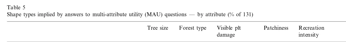
It is hardly surprising that the average most-and least-preferred levels in Table 4 are in the interior of the extent scales for each attribute (Table 1). Any other result would imply perfect agreement on these questions. But we believe it is important to note that for the most part, individ-ual respondents chose most-preferred levels that were themselves in the interiors of the extent scales (Table 5). Lower percentages chose interior least-preferred levels. We interpret this result as evidence that people gave some care to answering these questions, for it seems to us it would have been easier to have decided which direction was ‘better’ and just picked the better endpoint as most-preferred. (It is possible that some bias to-ward interior choices was introduced via the visu-als, which for the first four attributes did not
show the extremes, though levels close to the extremes were pictured. A micro-level examina-tion of the responses convinced us, however, that only for least-preferred tree size was this really a likely explanation. That is, choices did not line up with pictured levels for the most part.)
Interior most- and least-preferred levels do add a difficulty to the construction of the attribute-by-attribute sub-WTP functions that are central to the tests. This is because we have no information about the function ‘beyond’ an interior most-pre-ferred level. (Similarly, but, we believe, less
seri-ously for the region between an interior
least-preferred on the scale end beyond it.) Our solutions are described just below, and are opera-tionalized in Appendix A.
4.2. WTP and deri6ing the attribute-by-attribute WTP functions
iden-C
.
Russell
et
al
.
/
Ecological
Economics
36
(2001)
87
–
108
97
Table 5
Shape types implied by answers to multi-attribute utility (MAU) questions — by attribute (% of 131)
Tree size Forest type Visible plt Patchiness Recreation Extraction intensity
damage intensity
Percent with interior most preferred 78.6 93.9 84.7 80.1 87.7 77.9
51.9 21.4 16.1
Percent with interior least preferred 28.2 14.5 12.2
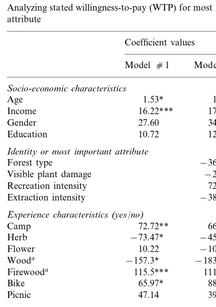
tified by a dummy variable. In model 1 this is not done. (The base case for this is the choice of either patchiness or tree size as the most important attribute. Only six people chose the former and one person the latter.)
From the responses to the questions about most- and least-preferred attribute levels, attribute weights, and WTP for the most important at-tributes, plus a linearization assumption, it is pos-sible to construct a set of attribute-by-attribute WTP functions (‘sub-WTP’ functions, for short). These allow us to infer the value, for any person,
Fig. 1.
of any forest as described by the six attributes. More to the point, they allow us to infer how each respondent should feel about the blended forests we asked about — preference direction for
each paired comparison; and his/her WTP for the
difference between the two.
The linearization is shown schematically in Fig. 1 for a response in which both an interior most-and least-preferred were chosen. This response form was the modal one for the intensity at-tributes. Generalizing to the other seven possible shapes is straightforward. The linearity assump-tion allows us to connect the WTP height of the function at the most-preferred attribute level to the zero WTP for the least-preferred level. (Recall that the question asked involves WTP for the difference between these two levels.) We further assume: that zero applies to all attribute levels beyond the stated least-preferred; and that the portion of the function beyond the most-preferred level and to the end of the scale may itself be linearized. The algebra for these calculations is set out in Appendix A.
4.3. Implied preferences and WTP for the blended forests
Using the sub-WTP functions we inferred pref-erences over, and WTP for diffpref-erences between, the blended forests described in Table 2. These results are reported in Tables 7a and 7b, parts (a) and (b).
4.3.1. Implied preferences
Our calculations of WTP for the three forests produce implied preference patterns favoring
Table 6
Analyzing stated willingness-to-pay (WTP) for most important attribute
Coefficient values
Modelc1 Model c2 Socio-economic characteristics
Age 1.53* 1.46*
Identity or most important attribute
Forest type −36.17
−2.76
Experience characteristics(yes/no)
Camp 72.72** 66.55*
Constant −160.4*** −162.6*
R2 0.216 0.262
0.143
AdjR2 0.166
Log likelihood −859.6 −855.5
F-stat 2.97 2.73
Prob (F-stat) 0.002 0.001
a‘Wood’ involves cutting wood for commercial purposes. ‘Firewood’ involves simply gathering wood for that purpose; not for sale.
* Significant atB15%. ** Significant atB10%.
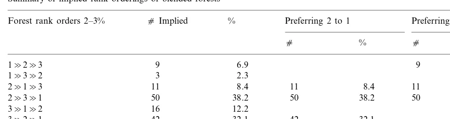
C.Russell et al./Ecological Economics36 (2001) 87 – 108 99 Table 7a
Summary of implied rank orderings of blended forests
% Preferring 2 to 1 Preferring 2 to 3 Forest rank orders 2–3% cImplied
c % c %
123 9 6.9 9 6.9
2.3 3
132
8.4 11 8.4
213 11 11 8.4
38.2 50 38.2
50 50
231 38.2
12.2
312 16
32.1 42 32.1
42 321
Total 131 100.1 103 78.7 70 53.5
Table 7b
Willingness-to-pay (WTP) calculated for each of the blended forests and the implied value of the difference between them ($/year; N=131)
Forest 1 Forest 2 Forest 3
Calculated mean WTP (BLENDi) $160.4 $215.4 $226.7
391.0 356.3
272.4 S.D.
Forest 2 vs. Forest 3 Forest 1 vs. Forest 2
Differences
−$11.3
−$55.0 Mean of signed differences
131.0
BLENDIi−BLENDIj S.D. 96.1
Mean of absolute differences $60.4 $42.5
BLENDIi−BLENDIj S.D. 128.6 86.8
forest 2. About 79% of respondents ‘should’ prefer forest 2 to forest 1; and 53.5% ‘should’ prefer forest 2 to forest 3. The implied pattern
found most often is 231 with 321 a
close second, so there is broadimplied agreement
that forest 1 is the least desirable (70.2% ‘should’ agree).
4.4. Implied WTP
Averaging implied WTPs for the differences among the forests across the sample gives a slightly different picture than the ‘vote count’ based on individual implied orderings. While in the aggregate forest 2 is valued at $55 per person per year over forest 1, forest 3 is implicitly valued more highly than 2 by the group, though the difference is only $11 per person per year. If the calculated values of the blended forests are taken to be drawings from a normal distribution, the mean calculated WTP difference between forests 1
and 2 is statistically significant; that between forests 2 and 3 is not.
For completeness, and because we will later examine absolute differences, we also report, in Table 7b, means of the unsigned differences in implied WTP for the forest differences.
4.5. Initial tests of the MAU ‘difference’
4.5.1. Intransiti6e responses to the blended forest preference questions
There was little evidence of confusion among respondents when they faced the three preference questions concerning the possible pairs of the three blended forests. Only 5 of 131 people (about 4%) gave responses implying intransitivity. We had expected more such responses. One practical and partial explanation is that in their stated preference responses, almost 60% of respondents selected forest 2 over both forest 1 and forest 3.
intransitivity and thus reduce the size of the set of
people who might exhibit confusion. That is, the
dominance of forest 2 may be in part responsible for the results. But only in part; 40% of respondents did not in effect ‘lock in’ transitivity.
This result tells us that at least by this measure and in this setting there is not much room for MAU
to ‘make a difference’. (The preferencesimpliedby
the MAU responses could never be intransitive.)
4.6. The extent of agreement between implied and stated preferences and WTP amounts
If the preference and WTP amounts implied by the answers to our MAU questions were in perfect agreement with those stated directly, MAU could be said merely to reproduce answers arrived at more directly. Zero agreement would mean that MAU makes a huge difference, though it would not be possible to claim that the MAU versions were ‘more correct’ than the direct statements. This is a reflection of the general problem of ‘verifying’ stated preferences or WTP results. Here, one might be inclined to suspect the MAU results, if only because of the importance of lin-earity to the method of deriving the sub-WTP relations for the attributes.
4.6.1. Agreement of implied and stated preferences
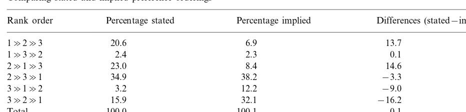
The implied preference orderings over the blended forests have already been reported. In Table 8 we compare the implied and stated pat-terns and the differences between the two (stated minus implied).
Informally, we see that, in the aggregate, the
orderings 123 and 213 are
under-pre-dicted; while 312 and 321 are
over-pre-dicted. Or, roughly speaking, the MAU
mechanism led us to infer that forest 3 was a good deal more popular than was consistent with the actual statements of individuals.
But these comparisons of aggregate counts could reflect massive mis-prediction at the level of the individuals, mis-predictions that, in effect,
cancel out.8 We therefore need to look at
individ-ual predictions and statements. One fairly
straightforward way to do this is to create a score variable according to the following rule:
Stated order Implied order Score
ijk 5
Using this scheme, we find results at the level of the individuals as shown in Table 9.
For a bit over a third of the sample, prediction and statement matched perfectly. For a bit over half, there was, at worst, a difference in ordering of the 2nd and 3rd ranked alternatives. And for almost three quarters, either the first and second or the second and third choices — but not both — were transposed.
Slightly less impressionistically, we can look at the correlation coefficients between the stated and implied preference relations for forests 1 and 2 and forests 2 and 3. These are both highly significant:
C.Russell et al./Ecological Economics36 (2001) 87 – 108 101 Table 8
Comparing stated and implied preference orderings
Percentage implied
Rank order Percentage stated Differences (stated−implied)
20.6
We can also calculate the Spearman rank order correlation to see whether the ranks (popularity) of the six possible full orderings are ‘close to’ being the same. For the comparison between stated and implied preference orderings, the calcu-lated correlation coefficient is 0.543 for six groups, which means that we can reject the null hypothesis of no relation between the orderings.
Finally, we can apply the McNemar test to compare the distributions of two related variables, using the numbers of matches and misses between stated and implied preference orders for the pairs considered separately. The key to this test is, in
effect, how big a difference there is between the
numbers of erroneous inferences: inferring 12
when the stated preference is the opposite; and
conversely inferring 21 when the stated
prefer-ence is the opposite. This explains why, even though the numbers of correct inferences are very close for the two comparisons (95 for 1 vs. 2 and 86 for 2 vs. 3) the test statistics are wildly different:
1 vs. 2 X2
=1.16 assymp. sig 0.281
assymp. sig 0.000
2 vs. 3 X2=24.03
So the null of no difference between the stated and implied orderings is not rejected for the 1 vs. 2 question, but is rejected for the 2 vs. 3 question, and we cannot say either that the MAU technique produces totally different answers or that it
closely mimics the summary judgments of
individuals.
4.6.2. Stated and implied WTP for differences between forests
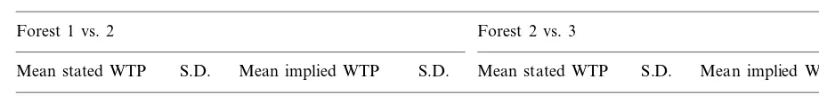
Above, we reported on the mean implied WTP for the differences between forests 1 and 2 and between 2 and 3. We now bring together the mean of stated WTP with the mean implied response in Table 10.
The differences between the stated and im-plied values for the two forest pairs are both significant at a level less than 5%. (A similar conclusion is reached using the Wilcoxon signed ranks test.)
4.6.3. Preference ordering analysis
What can be said about the relationship be-tween the level of agreement of stated and implied preference rankings over the blended forests and the characteristics of the respondents involved?
Table 9
Individual comparisons of stated and implied preferences over the blended forests
Cumulative % Score cof respondents %
5 44 34.9
Table 10
Mean stated and implied willingness-to-pay (WTP) for the difference between two blended forests (N=131) Forest 2 vs. 3
Forest 1 vs. 2
S.D. Mean stated WTP S.D. Mean implied WTP S.D. Mean stated WTP S.D. Mean implied WTP
$−11.3
$−19.9 133.9 $−55.0 131.0 $15.3 105.6 96.0
First, in order to keep the cell sizes up, we have simplified the score variable as follows:
Cell
To explore our ability to explain the score differences across individuals we tried both or-dered and sequential probit. The latter offered no improvement over the former, and in Table 11 only results of the former estimation exercises are reported. Neither the model using only the socio-economic variables nor the expanded version with all the experience variables is impressive in its
performance.9 In the first equation, education is
significant at less than 15% and the proportion of correctly predicted scores is 0.58. The expanded model has several significant coefficients — but none of those is attached to a socio-economic variable. It only does slightly better as a predictor of scores, with 0.60 correct. In neither case is any of the actual zero scores predicted; and in both there is substantial under-prediction of scores equal to one, while the number of scores equal to two is substantially over-predicted. It appears that our available information about the
respon-dents does not allow us to explain our failure to infer (from the MAU answers) the preferences across the blended forests that the respondents state.
4.6.4. WTP analysis
In Table 12 we summarize results from at-tempting to explain variations across respondents in the absolute size of the deviation between stated and implied WTP for the differences be-tween the blended forest. The forest 1, 2 and forest 2, 3 deviations are dealt with separately. (We examined models with only socio-economic explanatory variables, but these had very low
F-statistics and are not reported.)
For neither set of deviations are the explana-tory models very satisfacexplana-tory. For the forest 1, vs. 2 deviations, none of the socio-economic charac-teristics has a significant coefficient, though three of the experience dummies have coefficients sig-nificant at between 5 and 10% (camping,
fire-wood gathering, and ATV use). All these
coefficients are positive, suggesting that forest ex-perience somehow makes it more difficult for the MAU technique to infer the correct summary judgments across the multi-dimensional forests. Perhaps, for example, the experience leads people to formulate rules of thumb for judging forests — rules that are not adequately captured by the attribute-by-attribute, linearized MAU method.
The most interesting results are those for the forest 2 vs 3 deviations. The overall relation is
highly significant by the F-test, two of the
socio-economic variables are significant at between 5 and 10% (age and education), and two of the experience dummies are significant at least the 10% level. Again, all the significant coefficients are positive, suggesting that our MAU inferences
C.Russell et al./Ecological Economics36 (2001) 87 – 108 103 Table 11
Ordered probit analysis of modified score (implied vs. stated preference)N=126
Model 1 Model 2
Socio-economic6ariables
Age −0.0020 −0.0009
−0.0838
−0.0621 Income
−0.0879
Gender −0.0666
−0.0938 0.1307*1
Education
Experience6ariables
0.2308 Hike
Camp −0.0319
0.4211 Hunt
−0.6829***1 Herb
0.5511**1 Flower
Wood −0.0381
0.2207 Firewood
Drive 0.4084*1
Bike −0.3698
−0.7814 ATV
Picnic −0.0442
1.55***1
Constant 1.46***1
1.606
MU(1) 1.474
−106.2
Log likelihood −99.9
15.45 2.93
X2
15
Deg. free. 4
0.42 0.57
Significance
Frequency of correct prediction 73/126=0.58 75/126=0.60
Predicted
Actual Predicted Total actual
1 2 0 1
0 2
0 0 1 6 0 5 2 7
7 42 0
1 0 17 32 49
4 66 0
0 12
2 58 70
12 114
Total predicted 0 0 34 92 126
* Significant atB15%. ** Significant atB10%. *** Significant atB5%.
‘work’ better for younger, less well-educated re-spondents, and those with less active forest expe-rience. This has the virtue of being consistent with one of the arguments for using MAU tech-niques — that they are easier for people of mod-est experience and intellectual capacity to deal with.
5. The educational value of the MAU questions
instrument or really did demonstrate a greater ability to deal with multiple dimensions than peo-ple are usually given credit for, we administered a truncated survey without the MAU questions to 44 respondents. This survey went directly from a description of the attributes to the blended forest questions. Therefore, for this group of respon-dents, we do not have MAU answers from which to infer blended forest preferences and WTP. We only know what the respondents stated directly about their rankings of the blended forests and their WTP for the differences between them. The only meaningful comparisons are with those same statements from the respondents to the full sur-vey. Recall that the demographic characteristics of these two samples are similar, though the
Table 13
Comparison of stated blended forest preferences — full multi-attribute utility (MAU) and truncated survey samples
Truncated survey Rank orders Full MAU survey
(% stating) (% stating)
123 20.6 25.6
numbers involved are not large, and neither sam-ple mimics the population from which they were drawn.
The first important result is that only one of
the 44 people who responded to the truncated survey gave preference answers implying intransi-tivity. Thus, in the most obvious area for educa-tion to be helpful, no such effect is seen.
We can also compare stated preference rank-ings for the blended forests by the two groups (Table 13). The numbers certainly do not look very different. And using either the rank order correlation coefficient (0.943), or the Kendall tau –b (0.867), we find it possible to reject the null hypothesis of no relation with considerable
confidence (a=0.005 for the rank order test and
a=0.015 for the Kendall test).
And finally, we can look at stated (and signed) WTP amounts (Table 14). This comparison of stated WTP for forest differences conveys a mixed message. The means for the forest 1 vs. 2 comparison are almost identical. But the differ-ence between the sample means for the forest 2 vs. 3 comparison are different at a significant level less than 0.1%.
6. Concluding comments
The results of this experiment leave the reader free to judge the MAU glass either half full or
half empty, depending on his/her predisposition.
Someone positively inclined could stress that:
Table 12
Explaining absolute deviations between stated and implied willingness-to-pay (WTP) for the blended forest differences
Blended forest Blended forest c2 vs. c3 c1 vs. c2
Socio-economic characteristics
0.039 0.745**1
Firewood 55.76***1 36.66**1 16.59
Constant −92.66***1
R2 0.202 0.254
AdjR2 0.098 0.157
Log likelihood −807.9 −747.8 2.61 1.94
F-Stat
Prob (F-Stat) 0.026 0.002 * Significant atB15%.
** Significant atB10%.
C.Russell et al./Ecological Economics36 (2001) 87 – 108 105 Table 14
Comparison of stated willingness-to-pay (WTP) for differences between blended forests — full multi-attribute utility (MAU) and truncated survey samples
Forest 1 vs. 2 Forest 2 vs. 3
Full MAU (N=131) Truncated survey (N=43) Full MAU (N=131) Truncated survey (N=43)
Mean WTP S.D. Mean WTP
Mean WTP S.D. S.D. Mean WTP S.D.
−$20.8 218.5 $15.3 105.6 $56.1
−$19.9 133.9 230.9
It is possible to construct an MAU-based
sur-vey instrument, embodying multiple
indepen-dent dimensions of a complex valuation
problem (in our case, forests). The questions about preferences over the scale of each dimen-sion, relative importance of the dimensions (numerically expressed), and WTP to alter one of the dimensions can be answered, even by people with limited education.
Participants, who ranged in age from high
school students to volunteers from a nursing home, were generally quite willing to work through the tasks given to them and to think about valuation in the context of multiple at-tributes for a forest ecosystem. This positive result underlies the appeal of a constructive approach to valuation (Payne et al., 1992) and its fundamental assumption that our notions of value are built up, piece by piece, much as a building is constructed. Of course, some build-ings are built better than others, and protocols for the design of multi-attribute environmental evaluation efforts are still at an early stage (Gregory and Slovic, 1997). Nevertheless, the willingness of diverse respondents to undertake this rather lengthy task, and to stick with it through to a monetary valuation, suggests a fit between the way the questions were posed and how many participants naturally think about the types of policy questions that might affect management of a forest ecosystem.
Their answers, combined with a quite
restric-tive linearity assumption, allow the derivation of a ‘sub-WTP function’ for each dimension or attribute. These functions can, in turn, be used to infer at least relative values for the particu-lar multi-dimensional good at issue (here
forests) described by combinations of the at-tributes. In particular, it is possible to make judgments among alternative possible goods, either on the basis of ‘votes’ (aggregating ordi-nal preferences) or total WTP.
The inferred preferences and WTP figures
ap-proximate, though they do not perfectly match, the stated preferences and WTP numbers ob-tained directly from respondents.
The stated WTP answers themselves appear, in
general, to be sensibly related to key socio-eco-nomic characteristics of the respondents. But a more skeptical person might question the importance of these findings by pointing to some awkward facts.
It is not clear that the MAU process makes
much difference in the chosen setting, multi-di-mensional though it is, because: (i) a subsample
asked for blended forest preferenceswithoutthe
benefit of the MAU educational process exhib-ited even less cyclicity (taken as evidence of confusion about the vector comparisons); (ii) the mean WTP answers of this group for the differences between blended forests were in one case identical to the mean from the ‘educated’ sample and in one case different; (iii) the stated preference orderings over the blended forests were not significantly different for the unedu-cated and eduunedu-cated samples.
Thus, it may be that MAU could be useful in
more complex problem settings, for which the
vector comparisons would be overwhelming — if
there were more dimensions, for example. But the skeptic might well say, in addition, something along the following lines:
Even granting that each question is quite
took a long time to complete (so was almost certainly not a good candidate for a mail sur-vey, which in turn implies the technique may be expensive to use; (ii) only 75% of those who sat down to do the survey successfully (com-pletely) finished.
The several stated WTPs are about the only
results that seem to ‘make sense’, if the test is: can we explain the variation across respondents by their characteristics and self-reported expe-riences (with forests)? In particular, there ap-pears to be no straightforward explanation of variation in the matches between implied and predicted preferences and WTP numbers for the blended forests pairs.
So, it seems clear that the jury is still out on the promise of MAU as an alternative to the conven-tional contingent valuation technique for prob-lems such as ecosystem valuation. The approach cannot be rejected as without promise. But neither can it be embraced as the answer to the problems of cognitive challenges — especially multi-dimen-sionality — identified in the literature and likely to become more common as the boundaries of the search for dollar values in the environment are pushed out by the needs of policymakers.
How might one extend the investigation of the potential for the MAU survey technique? Our recommendations are aimed at avoiding some of the difficulties observed in this study, and increas-ing the chance of findincreas-ing a definitive result.
First, it would seem desirable to concentrate on
attributes that are believably ‘manageable’. If an attribute is clearly the result of natural forces and events, respondents may wonder what the point of asking about their prefer-ences is.
Second, we would suggest a method of survey
administration, perhaps via laptop computers or using an Internet sampling company such that each person could be offered a randomly designed set of multidimensional ‘forests’ (or wetlands or streams, or whatever) to answer preference and WTP questions about. This would avoid the ‘dominance’ problem that is reflected in our intransitivity results.
Finally, as almost goes without saying, we
would push for enough funding to produce
completed surveys in at least the 8009 range
rather than the 2009 managed here. This
might be achieved by simplifying the questions even more than we managed, so that a cheaper ‘delivery’ method would be possible.
Appendix A. Deriving the parameters of the ‘Sub-WTP’
A.1. Functions from sur6ey responses
Successfully completed surveys contain the fol-lowing information:
most- and least-preferred levels of each
attribute
importance ranks and associated weights for
the attributes
stated WTP of each respondent to change her/
his most important attribute from her/his
least-to most-preferred level.
The exposition here will be notationally simpler if we use subscripts to indicate order of attribute importance rather than order in the list of at-tributes. So let us call the basic data:
most- and least-preferred levels of the attribute
that is ith in descending order of importance:
bM
i ,b
L i
importance weight for the ith attribute: wi
WTP for the most important attribute: P1
Two important relations may be inferred from the way the WTP and the weight questions are asked.
C.Russell et al./Ecological Economics36 (2001) 87 – 108 107
where the a
i are scaling constants, and Z is
income.
Define bM
i −b
L
i=Dbi
For the weights, it must be true that:
wia1Db1=aiDbi
Now: P1=a1Db1, which in effect, defines a1.
But, it must be true that there are also in principle
P2, . . .,P6 that could have been obtained from
respondents by questions of the form asked for
P1. Thus, Pi=wiaiDbi would be true.
This allows us to construct estimates for thePi,
based on P1 and the other known parameters.
Thus,
where the hat indicates that we are estimating the attribute WTP rather than recovering it from a statement. In terms of what we call the attribute WTP functions, then, we have the height of the
functions at the attribute values bM
. The slope of
the function between bM
i and b
which is positive whenbM
i is to the right (higher)
on the attribute scale. The WTP for some level of
bi, call it b
numerator of the second term in the brackets is negative, while the denominator is positive. Vice
versa, for the case in which bL
i is to the right of
bM
i .
Finally, in calculating the WTP for the blended forests, it is necessary to allow for cases in which the actualba
i falls outside theb L
i tob
M
i range. The
rules used here are:
Ifbai is ‘on the other side’ ofbLi from the most
important level, Pi(ba
i) for that attribute is
zero.
If thebai is ‘on the other side of’ the
most-pre-ferred point from the least-premost-pre-ferred, then we
linearize the function so that it’s slope is Pi/
(bM
right-hand end of the scale and b6 the left-hand
end.)
References
Bergland, O., 1994. Valuing Multidimensional Changes with Contingent Ranking, Discussion Paper D-15/1994, Depart-ment of Economics, Agricultural University of Norway, A,s, Norway.
Bohm, P., 1994. CVM spells responses to hypothetical ques-tions. Nat. Resources J. 34 (winter), 37 – 50.
Coss, R.G., Moore, M., 1990. All that glistens: water connota-tions in surface finishes. Ecol. Psychol. 2, 367 – 380. Edwards, W., 1977. Use of multi-attribute utility measurement
for social decision making. In: Bell, D., Keeney, R., Raif-fer, H. (Eds.), Conflicting Objectives in Decisions. John Wiley, New York.
Fischhoff, B., 1991. Value elicitation: is there anything in there? Am. Psychol. 46, 835 – 847.
Fishkin, J., 1995. The Voice of the People. Yale University Press, New Haven.
Gregory, R., Slovic, P., 1997. A constructive approach to environmental valuation. Ecol. Econ. 21 (3), 175 – 182. Gregory, R., Lichtenstein, S., Slovic, P., 1993. Valuing
envi-ronmental resources: a constructive approach. J. Risk Un-certainty 7, 177 – 197.
Hanley, N., Ruffell, R.J., 1993. The contingent valuation of forest characteristics: two experiments. J. Agric. Econ. 44 (2), 218 – 229.
Hanley, N., R.E. Wright, and V. Adamowicz, 1997. Using choice experiments to value the environment: design issues, current experience, and future prospects. Unpublished, re-submitted to a special issue of Environmental and Re-source Economics.
Hobbs, B., Horn, G., 1997. Building public confidence in energy planning: a multi-method MCDM approach to demand-side planning at BC gas. Energy Policy 25, 357 – 375.
Jenni, K.E., M.W. Merkhofer, and C. Williams, 1994. The Rise and Fall of a Risk-Based Priority System: Lessons from DOE’s Environmental Restoration Priority System. Discussion paper, unpublished, Applied Decision Analysis, Menlo Park, CA.
Kaplan, R., Kaplan, S., 1989. The Experience of Nature: A Psychological Perspective. Cambridge, New York. Keeney, R.L., 1992. Value-Focused Thinking: A Path to
Cre-ative Decision-Making. Harvard University Press, Cam-bridge, MA.
Keeney, R., Raiffa, H., 1976. Decisions with Multiple Objec-tives: Preferences and Value Tradeoffs. Wiley and Sons, New York.
Southeast Loblolly/Shortleaf Pine Demonstration Interim Report. United States Environmental Protection Agency, Environmental Monitoring and Assessment Program Cen-ter, Research Triangle Park, N.C., Report EPA/620/SR – 94/006.
Merkhofer, M.W., Keeney, R.L., 1987. A multi-attribute util-ity analysis of alternative sites for the disposal of nuclear waste. Risk Anal. 7 (2), 173 – 194.
Miller, G.A., 1956. The magical number seven, plus or minus two: some limits on our capacity for processing informa-tion. Psychol. Rev. 63, 81 – 97.
Mitchell, R., Carson, R.T., 1984. A Contingent Valuation Estimate of National Freshwater Benefits: Technical Re-port to U.S. EPA. Washington, DC: Resources for the Future.
Mitchell, R., Carson, R.T., 1989. Using Surveys to Value Public Goods: The Contingent Valuation Method. Re-sources for the Future, Washington, DC.
Payne, J., Bettman, J., Johnson, E., 1992. Behavioral decision research: a constructive processing perspective. Annu. Rev. Psychol. 43, 87 – 131.
Phelps, R.H., Shanteau, J., 1978. Livestock judges: how much information can an expert use? Organ. Behav. Hum. Per-form. 21, 209 – 219.
Russell, C.S., V. Dale, J. Lee, M.H. Jensen, M. Kane, and R. Gregory, 1997. Applying Multi-Attribute Utility Tech-niques to Environmental Valuation: A Forest Ecosystem Example. Final Project Report to the Environmental Pro-tection Agency, December.
Saaty, T., 1983. Priority setting in complex problems, IEEE Trans. Eng. Manage., EM-30, August.
Schkade, D., Payne, J., 1994. How people respond to contin-gent valuation questions: a verbal protocol analysis of willingness to pay for environmental regulation. J. Envi-ron. Econ. Manage. 26 (1), 88 – 109.
von Winterfeldt, D., 1987. Value tree analysis: an introduction and an application to offshore oil drilling. In: Kleindorfer, P., Kunreuther, H. (Eds.), Insuring and Managing Haz-ardous Risks: From Seveso to Bhopal and Beyond. Springer-Verlag, New York, pp. 349 – 377.
von Winterfeldt, D., Edwards, W., 1986. Decision Analysis and Behavioral Research. Cambridge University Press, Cambridge.