Impact of household consumption on CO
2emissions
Jesper Munksgaard
a,U, Klaus Alsted Pedersen
a,
Mette Wien
a,b aAKF, Institute of Local Go¨ernment Studies, Nyropsgade 37, DK-1602 Copenhagen, Denmark
b
National En¨ironmental Research Institute, Department of Policy Analysis, P.O. Box 358, DK-4000 Roskilde, Denmark
Abstract
Danish household consumption increased by 58% over the period 1966]1992 while CO2 emissions only increased by 7%. Using decomposition analysis we investigated the global CO impact of Danish household consumption from 1966 to 1992. Our conclusion is that2 overall growth in private consumption }but not changes in the composition of consump-tion }is the key to understanding the increase in CO emissions. However, the effect of2 growth in private consumption has been partly offset by substantial energy conservation in the energy supply and manufacturing sectors. Q 2000 Elsevier Science B.V. All rights reserved.
JEL classification:Q40
Keywords:CO ; Household consumption; Decomposition analysis2
1. Introduction
The Danish Government’s energy action plan ‘Energy 21’ sets the ambitious goal
Ž
of reducing CO emissions by 20% in 2005 compared to the 1988 level Ministry of2
.
Environment and Energy, 1996 . However, it has proven difficult to control CO2 emissions which have only decreased by 4% between 1988 and 1996. Danish consumers are partly responsible for this.
U
Corresponding author. Tel.:q45 33 11 0300; fax:q45 33 15 2875.
Ž . Ž . Ž .
E-mail addresses:[email protected] J. Munksgaard , [email protected] K.A. Pedersen , [email protected] M. Wien . 0140-9883r00r$ - see front matterQ2000 Elsevier Science B.V. All rights reserved.
Ž .
In the present article we focus on CO2 emissions associated with private consumption. Our main point is that changing consumer habits and household demand towards more environmental detrimental commodities represents the main challenge with respect to CO emission reduction targets.2
Using structural decomposition analysis, we have analysed the factors affecting the development in CO emissions from private consumption over the period2 1966]1992, distinguishing between direct and indirect CO emissions. Direct CO2 2 emissions are generated by direct household energy use whereas indirect CO2 emissions are generated in the industrial sectors producing non-energy commodi-ties demanded by the households. The study thus examines the influence of both consumer behaviour and behaviour of the firm.
The article decomposes CO emissions from Danish household consumption at2 the global level, i.e. emissions from imported commodities as well as commodities produced in Denmark are taken into account. The reason for doing so is that Danish consumers are responsible for the global environmental consequences of their consumption.1
Section 2 below describes the model and methodology while Section 3 describes the data applied and Section 4 reports the results of the analysis. Finally, Section 5 summarises the conclusions.
2. Model and methodology
Over the past decade, decomposition analysis has proved to be a useful tool for
Ž
analysing changes in energy consumption e.g. Boyd et al., 1988; Chen and Rose, 1990; Li et al., 1990; Rose and Chen, 1991; Liu et al., 1992; Lin and Polenske, 1995;
.
de Bruin et al., 1996 . A few studies have also decomposed changes in emissions
Že.g. Halvorsen et al., 1991; Common and Salma, 1992; Ang and Pandiyan, 1997;
.
Chang et al., 1998 .
With regard to Danish data, decomposition analysis has been applied to changes
Ž .
in energy consumption from production Howarth et al., 1993; Pløger, 1984 ,
Ž .
changes in CO emissions Torvanger, 1991 and changes in CO , SO and NO2 2 2 x
Ž .
emissions from production Wier, 1998 . Finally, changes in nitrogen loading from agricultural and industrial production have been decomposed by Wier and Hasler
Ž1999 ..
In the present study, decomposition addresses the production sectors as well as the household sector. Compared to the studies mentioned above, this study distinguishes itself by two important features: Firstly, it includes the households’ direct demand for energy and secondly, it handles changes in commodity mix in private consumption at a highly disaggregated level, encompassing 66 commodities.
1
In addition, the Danish data sets used are very comprehensive, covering 117 production sectors, 30 types of energy and 66 commodities, and the analysis period is very long, namely from 1966 to 1992.
The model applied is an extended input]output model based on Danish input-output tables plus energy flow matrices and CO emission factors. These can be2 linked together due to the use of common classifications. The strength of the model is that it covers all sectors of the economy and operates at a very disaggregated level. Moreover, it covers the entire energy production and consump-tion cycle, and is able to distinguish between direct and indirect uses of energy.
In the present study we focus on total CO emissions associated with Danish2 household consumption, distinguishing between direct and indirect emissions. The direct emissionsare emissions associated with the consumption of energy commodi-ties in the households, i.e. electricity, district heating, gas and other liquids. The indirect emissions are emissions associated with the production of all other com-modities for households, i.e. emissions that takes place in the industry producing furniture, food, clothes, services etc. used in households.
Fig. 1 illustrates the basic model. Note that also deri¨ed emissions, i.e. emissions
Ž .
associated with direct and indirect production of inputs are included.
Fig. 1. Direct and indirect CO emission.2
Total CO emissions are defined as2
Ž .
where
E is total CO emissions from households;2 Eh is direct CO emissions from households; and2 Ep is indirect CO emissions from households.2
The decomposition analysis is carried out in two steps. First, direct CO2 emissions from household energy use are analysed using a simple energy emission model. Second, indirect CO emissions are analysed using an extended input2 ] out-put model that also incorporates energy and emission matrices.
2.1. Decomposition of direct CO emissions2
Ž .
Model 2 below estimates direct CO emissions from household energy use as a2 product of total energy consumption and the composition of energy types in the household and energy supply sectors.
Ž .
EhsQ M Fh h 2
where:
Eh denotes a scalar of total direct CO emissions from households;2
Qh is a 1=5 vector including the absolute level of five categories of household
energy consumption, i.e. electricity, gas, oil, gasoline and other heating
Žprimarily district heating, coke and coal ;.
Mh is a 5=30 matrix of fuel mix in the household sector, i.e. demand for 30 energy types per unit of total energy demand for five energy consumption categories; and
Ž
F is a 30=1 vector of CO2 emissions per unit for 30 energy types cf. .
Appendix A . The emission factors are constant for 27 of the 30 types of energy as they solely depend on the carbon content of the fuel. For three
Ž .
types, however electricity, district heating and gas from gasworks the CO2 emission factor depends on fuel mix in the energy supply sector, and consequently changes over time.
Ž .
According to model 2 , direct CO emissions depend on changes in the factors2 Qh, Mh and F. The decomposition analysis is carried out by changing the factors one-by-one in order to quantify the contribution of each factor to total change in emissions. The contribution of each factor, e.g. Qh, is estimated as the change in
Ž . Ž .
the factor DQh multiplied by the other factors Mh and F . The other factors may figure at base-level or at current-year level, however. Thus all changes may be weighted using either base-year values for the other two factors or current-year values. Both approaches cause considerable bias, however. This can be overcome,
Ž .
using structural decomposition analysis as introduced by Fujimagari 1989 and
Ž .
average of the two approaches.2 Thus, the total change in emissions from time ty1 until time t is
Ž . Ž . Ž .
E th yE th y1 sDQhqDMhqDF 3
where:
DQh is the effect of changes in household energy consumption level;
DMh is the effect of changes in the composition of energy types in household energy consumption; and
DF is the effect of changing emission factors, i.e the effect of fuel mix changes in energy production.
Each element in the decomposition formula has the same general form. For reasons of brevity, only one effect } the effect of fuel mix changes in households
ŽDMh. } is used as an example:
Ž .w Ž . Ž .x Ž .
DMhs1r2Q th y1 M th yM th y1 F t
Ž .w Ž . Ž .x Ž . Ž .
q1r2Q th M th yM th y1 F ty1 3a
2.2. Decomposition of indirect CO emissions2
Ž .
Model 4 below estimates the indirect CO emissions from household consump-2 tion by using the extended input]output model as introduced by Leontief and Ford
Ž1972 ..
y1 N
Ž . Ž . Ž .
EpsF MpaRp IyA C c c 4
where:
a denotes element by element multiplication
Ep denotes a scalar of total indirect CO emissions in production sectors as2 a consequence of production of goods for household consumption; F is a 30=1 vector of CO emissions per unit of consumption of each of2
the 30 energy types;
Mp is a 30=117 matrix of fuel mix in the production sectors, i.e. demand for 30 energy types per unit of total demand for energy for all produc-tion sectors;
Rp is a 1=117 vector of energy intensities, i.e. total energy consumption
per unit of production in all 117 sectors;
2
The choice of decomposition method is a question of choosing how to handle the interaction effect i.e. that part of total change for which no single factor is responsible. There is no unambiguous and correct way to handle the interaction effect, and several approaches have been applied during the last decade. Some of these apply different indices, of which the Divisia based index approach is the most
Ž . Ž . Ž .
ŽIyA.y1 is the 117=117 Leontief inverse matrix;
C is a 117=66 matrix of the composition of consumption commodity aggregates, i.e. 66 private consumption commodity aggregates appor-tioned by production sectors;
c is 66=1 vector of aggregate commodity mix in private consumption, i.e.
demand for 66 commodities per unit of total consumption; and cN denotes a scalar of total private consumption.
Ž .
According to model 4 , indirect CO emissions change as a consequence of2
Ž .y1 N
changes in seven factors: F, Mp, Rp, IyA ,C, c, and c . Whereas C, c, and cN are factors of consumer behaviour, i.e. demand for consumption commodities,
Ž .y1
F,Mp, Rp, IyA are factors of behaviour of the firm, i.e. demand for inputs in the energy supply sector and other production sectors.
The total change in emissions from time ty1 until time t is
y1 N
DF is the emission factor effect or effect of fuel mix changes in energy
.
production ;
DMp is the effect of fuel mix changes in the production sectors; DRp is the effect of changes in energy intensities;
Ž .y1
D IyA is the input mix effect;
DC is the effect of changes in mix within aggregated commodities; Dc is the effect of changes in mix between aggregated commodities in
private consumption; and
DcN is the effect of change in total consumption level.
Again, each element in the decomposition formula has the same general form.
Ž .
Using the effect of changes in energy intensity DRp as an example, this element is whereadenotes element by element multiplication.
3. Data
The data used for the analysis are:
Žtables documented in Statistics Denmark, 1986 . The tables encompass 117.
production sectors and nine categories of final demand. One of the latter is private consumption, which is divided into 66 components, five of which are direct energy consumption by households.
v Energy-flow matrices for the years 1966]1992 from Statistics Denmark contain-ing energy consumption for the 117 production sectors as well as for five
Ž
categories of household consumption matrices documented in Statistics
Den-.
mark, 1983 . Energy demand is reported for 25 types of energy in both monetary, physical and calorific terms. The latter is used in the present study as emission factors are given relative to calorific terms.
Ž .
v Supplementary statistics of renewable energy wood, straw, refuse and others
Ž .
from Ministry of Environment and Energy Danish Energy Agency, 1997 . The energy flows from Statistics Denmark lack a complete inventory of renewable energy, which underestimates energy consumption by households and power plants. For present purposes the energy flow matrices from Statistics Denmark have been extended with data on consumption of renewable energy, increasing
Ž .
the number of energy types from 25 to 30 cf. Munksgaard et al., 1998 . v CO2 emission factors for the 22 primary fuels are part of the European
Ž .
CORINAIR database Fenhann et al., 1997 . The factors are calculated on the basis of the carbon content of the fuels. Emission factors for the converted
Ž .
energy types electricity, district heating and gas have previously been calcu-lated from the primary emission factors and the energy inputs to the energy
Ž .
production sector Munksgaard et al., 1998 . Finally, CO emission factors for2 renewable energy types are considered to be zero, as it is assumed that CO2 emissions from, e.g. straw and wood are absorbed in new biomass production.
While the data concerning input]output tables and CO emission factors are2 quite robust, there is some uncertainty associated with some of the energy flows, especially during the period 1966]1975. Moreover, the description of joint produc-tion of heat and electricity in power plants suffers from some weaknesses concern-ing estimation of input demand.
In the Danish input]output tables, no specific knowledge on foreign technology is incorporated. Thus, with regard to imported goods, an important assumption is made: Foreign technology is assumed to be identical to Danish technology. This assumption entails considerable uncertainty, as 20% of the total CO emissions2
Ždirect and indirect from households take place abroad.. 3
4. Results
Direct and indirect household CO emissions increased by 7% from 38.6 million2 tonnes in 1966 to 41.4 million tonnes in 1992. The indirect emissions accounted for
Ž .
a major part of this growth} 2.5 million tonnes 15% , while the direct emissions
Ž .
although the difference has been diminishing. In 1992, direct emissions thus accounted for 21 million tonnes whereas indirect emissions accounted for 20 million tonnes.
Main emission changes and the driving forces are highlighted in the household CO emission account in Table 1. As is apparent from the table, the stable direct2 CO emissions hide two major trends: a sizeable growth in energy consumption2 and changes in household fuel mix which have partly offset this growth. The increase in indirect CO emissions is primarily due to the general growth in private2 consumption, whereas substantial energy conservation having reduced energy in-tensity in most production sectors.
For reasons of brevity, the results of the decomposition analysis of direct and indirect CO emissions are reported in Sections 4.1 and 4.2 below at a highly2 aggregated level. However, information from decomposition performed at a more
Ž .
disaggregated level Munksgaard et al., 1998 is referred whenever needed and some detailed results based on commodity groups are examined in Section 4.3.
4.1. Direct CO emissions2
As is apparent from Table 2, direct CO emissions remained rather stable over2 the period 1966]1992 although there was a substantial increase from 1966 to 1976, mainly due to increasing household energy consumption. During the 1970s, how-ever, substantial energy conservation and shifts towards less polluting fuels modi-fied this effect.
A further decomposition analysis shows that especially demand for electricity and gasoline has increased. Electricity demand has increased continuously through-out the period due to the introduction of household electrical appliances.
From mid 1970s, major energy conservation measures were introduced in the household sector as a consequence of the rising oil and gasoline prices in 1973 and 1978. This gave house owners an incentive to insulate walls and roofs and led the construction sector to develop low-energy residential buildings. From the mid-1970s, energy efficient district heating and natural gas were introduced in many single family homes instead of oil fired heating systems. Moreover, gasoline consumption decreased by 22% between 1978 and 1983. From 1983 to 1992, however, gasoline consumption increased by 37%. Thus in the 1990s, increasing demand for
electric-3 Ž .
Table 1
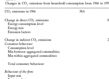
a Changes in CO emissions from household consumption from 1966 to 19922
CO emissions in 19662 38.6
Change in direct CO emissions2 q0.1
Energy consumption level q3.9
Energy mix y2.9
Emission factors y0.9
Change in indirect CO emissions2 q2.6
Consumer beha¨iour:
Consumption level q8.3
Mix between aggregated commodities y0.7
Mix within aggregated commodities q0.1
Total consumer behaviour q7.7
Beha¨iour of the firm:
Input mix 0.0
Emission factors y0.1
Energy mix q0.5
Energy intensity y5.5
Total behaviour of the firm y5.1
CO emissions in 19922 41.4
a
Note:The discrepancy in the sum is due to rounding off of decimal places in the individual figures.
ity and gasoline may threaten future attempts to control CO emissions from the2 household sector.
Changes in household fuels had little impact on CO emissions, except from2 1966 to 1977. During this period, most single family homes installed oil fired central heating systems instead of coal and coke ovens. The overall effect was a 13.7% decrease in emissions. Changes in fuel composition in the energy production
Table 2
Decomposition of direct CO emissions2
Period Energy Energy mix Emission Total
consumption factors
level
1966]1971 20.2% y6.2% y2.1% 11.9%
1971]1976 8.9% y0.2% 0.7% 9.4%
1976]1981 y9.3% y1.7% 2.5% y8.5%
1981]1986 0.8% y0.4% y1.9% y1.5%
1986]1992 y5.2% 0.3% y3.8% y8.8%
Ž .
sector also reduced CO emissions, but only to a small extent 4.3% . Emissions2 decreased until the early 1970s, whereafter they increased until the mid-1980s. Since then CO emissions have decreased continuously. The explanation is that2 until the first oil crisis in 1973, power plants were substituting oil for coal. As coal is more CO intensive, this was environmentally beneficial. After the oil crisis,2 however, the power sector substituted from oil to coal, consequently enhancing CO emissions. Since the mid-1980s, a higher share of natural gas, straw and refuse2 in energy production has ensured a total decline in emissions. Increased efficiency in the energy sector from increased co-production of heat and power has also contributed to the reduction in CO emissions.2
4.2. Indirect CO emissions2
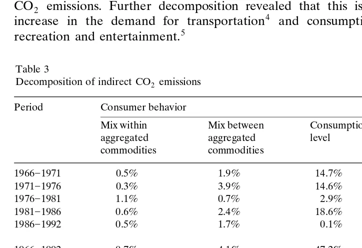
The indirect CO emissions from household consumption increased by 15%2 from 1966 to 1992, as shown in Table 3.
Most of the growth can be explained by the increasing level of private consump-tion, especially during the periods 1966]1976 and 1981]1986. Over the whole period 1966]1992, growth in the level of consumption generated a 47% increase in CO emissions. Further decomposition revealed that this is mainly due to an2 increase in the demand for transportation4 and consumption associated with recreation and entertainment.5
Table 3
Decomposition of indirect CO emissions2
Period Consumer behavior Total
Mix within Mix between Consumption
aggregated aggregated level
commodities commodities
1966]1971 y0.5% y1.9% 14.7% 16.8%
1971]1976 y0.3% y3.9% 14.6% y1.8%
1976]1981 1.1% 0.7% y2.9% y2.9%
1981]1986 0.6% y2.4% 18.6% 9.5%
1986]1992 0.5% 1.7% 0.1% y5.7%
1966]1992 0.7% y4.1% 47.2% 15.0%
Behaviour of the firm
Input mix Emission Energy mix Energy
factors intensity
1966]1971 9.4% y2.9% 0.6% y2.6%
1971]1976 y10.1% 1.6% 1.2% y4.8%
1976]1981 3.3% 2.9% 2.9% y10.9%
1981]1986 y3.1% y0.4% 0.0% y3.7%
1986]1992 0.8% y1.1% y0.4% y7.4%
The second most important factor is reduced energy intensity, which generated a 31% decrease in emissions over the period 1966]1992. Many energy conservation projects were implemented during this period, especially in the second half of the 1970s after the oil crisis6.
During the periods 1976]1981 and 1986]1992, growth in the overall level of consumption was rather stable, partly due to reduced consumption of clothing and cars, and CO emissions consequently decreased. This was also the case for the2 period 1971]1976, as changes in input mix and energy conservation in production sectors together with changes in commodity mix in households resulted in an overall total decline in CO emissions2 } despite considerable growth in private consumption. Generally speaking, however, structural effects, i.e. changes in input mix, energy mix, and commodity mix have had little impact.
4.3. Intensity of commodities for household consumption
Changes in household commodity mix reduced CO emissions by 4.1%. While2 this effect is minor, analysis at the detailed commodity level shows that the CO2 effects from changes in commodity mix was substantial. CO2 emissions from private consumption during the period 1966]1992 are shown for eight aggregated commodity groups in Table 4. Detailed CO intensities for different commodities2 are shown in Appendix B.
CO2 emissions associated with the consumption of clothing and household
Ž .
appliances including operation decreased by 30% and 10%, respectively, between 1966 and 1992. Emissions associated with consumption of the remaining commodi-ties increased in some cases significantly. Thus, emissions from the consumption of
Ž
services mail and telecommunications, law and financial services, private teaching
.
and day-care increased by 234%, while emissions from consumption of recreation
Ž
increased by 59% and emissions from transportation vehicles and purchased
.
transport services increased by 54%.
Emissions from consumption of a given commodity may change as a conse-quence of changes in consumption of the commodity andror changes in CO2 intensity, i.e. the direct and indirect CO emissions from consuming and producing2 the commodity. Consumption and CO intensity are shown for the commodity2 groups in Table 5.
In 1966, food, beverages and tobacco, and clothing were thus the most CO2
Ž .
intensive commodity groups Table 5 . In 1992, transport took the lead together
4
Transport covers consumption of vehicles, public transport, taxis, and freight purchased by house-holds. Note that consumption of gasoline is not included } it is encompassed by direct household energy consumption.
5
Entertainment covers manufacturing of recreational goods, entertainment, cultural services, media consumption, etc.
6
Table 4
Ž .
CO emissions in 1966 and 1992 by commodity groups million tonnes CO2 2
Commodity group 1966 1992 Change in emissions
Foods 5.5 5.5 1%
Beverages and tobacco 0.8 1.0 25%
Clothing 2.3 1.6 y30%
Household appliances 3.2 2.8 y10%
incl. operation
Health 0.6 0.7 18%
Recreation and enter- 2.4 3.9 59%
tainment
Services 0.3 1.1 234%
a
Transport 2.0 3.0 54%
a
Includes vehicles and public transport services.
with foods and beverages and tobacco. Comparison of changes in CO intensity2 and consumption reveals that the sizeable growth in emissions from services, recreation and entertainment, and transport is not due to changes in emission intensity since the emission intensity of transport has only increased by 5%, while that for services and recreation and entertainment has decreased by no less than 8% and 25%, respectively. Emission growth is due to increasing consumption of all of these commodity groups, and is partly offset by reduced CO intensity.2
The highest growth rates are observed in the consumption of services, transport, and recreation and entertainment. This indicates changing consumption patterns towards a life style with more telecommunications, more travelling and more leisure activities. From an environmental point of view this development is mainly
Table 5
Consumption and CO intensity for different commodity groups2
Ž
Commodity group Consumption thousand CO intensity2
. Ž .
million 1980-DKK kgrDKK
1966 1992 Change 1966 1992 Change
Foods 26.6 34.4 28% 0.20 0.16 y22%
Beverages and 4.2 6.6 46% 0.20 0.16 y21%
tobacco
Clothing 13.4 13.7 2% 0.17 0.12 y31%
Household appl- 33.9 55.5 54% 0.09 0.05 y45%
Ž
iances incl.
opera-.
tion
Health 4.9 7.4 50% 0.12 0.10 y22%
Recreation and 15.5 32.8 94% 0.16 0.12 y25%
entertainment
Services 4.6 16.5 196% 0.07 0.07 y8%
a
Transport 11.7 17.1 39% 0.17 0.18 5%
a
beneficial since services and recreation and entertainment are characterised by low CO intensity. However, the increasing demand for transport services may consti-2 tute a severe problem in the future and considerable efforts should therefore be made to control CO emissions from this activity.2
As shown in Table 4, emissions from the consumption of foods accounted for 5]6 million tonnes CO per year during the period 19662 ]1992. Consumption of foods is responsible for more than 10% of total Danish CO emissions from the2 household sector. Comparison of indirect and direct household emissions reveals
Ž
that only emissions associated with electricity consumption 8 million tonnes CO2
.
per year are greater than those associated with the consumption of foods. In comparison, gasoline consumption only accounts for 5 million tonnes CO . One2 should, therefore, bear in mind that CO emissions can be influenced in many2 ways. Controlling private transport is just one possibility, while creating incentives for energy savings in food production is another. Trying to influence life style and consumption habits is a third approach.
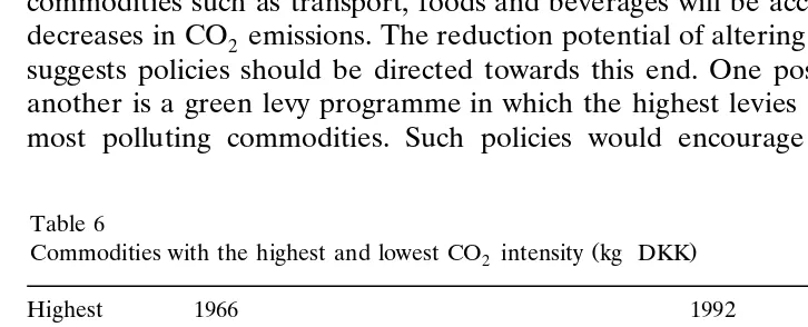
In fact, policies directed towards household consumption of commodities other than energy offer considerable potential for reducing CO2 emissions. As the differences in the CO intensity of the various commodities is sizeable, changes in2 commodity mix towards less CO intensive goods could be of significant impor-2 tance. Table 6 illustrates the large variation in CO2 intensity, listing the five commodities with the highest and lowest CO intensity in 1966 and 1992.2
In 1992, the most CO intensive commodity was transport which is very energy2 intensive. Second came public transport, followed by various food products. The five commodities with the lowest CO intensity are various types of services. This2 implies that greater demand for services together with reduced consumption of commodities such as transport, foods and beverages will be accompanied by major decreases in CO emissions. The reduction potential of altering the commodity mix2 suggests policies should be directed towards this end. One possibility is labelling, another is a green levy programme in which the highest levies are imposed on the most polluting commodities. Such policies would encourage the consumers to
Table 6
Ž .
Commodities with the highest and lowest CO intensity kg2 rDKK
Highestr 1966 1992
lowest
Top 5 Fruit and vegetables 0.38 Transport 0.30
Sport and camping equipment 0.33 Margarine etc. 0.22
Sugar 0.30 Other foods 0.22
Wine and liquor 0.30 Fruit and vegetables 0.21
Margarine etc. 0.28 Sugar 0.20
Bottom 5 Life insurance etc. 0.05 Education 0.06
Health and accident insurances 0.05 Medical care 0.05
Housing 0.04 Housing 0.03
Private organisations 0.03 Private organisations 0.03
spend more of their budget on services and other commodities with low CO2 intensity. However, the impact of a green levy programme will depend on how price elastic the demand is.
5. Concluding remarks
Overall growth in household consumption of energy as well as other commodi-ties was found to be the main driving force behind growth in CO emissions over2 the period 1966]1992. This was partly offset by reduced energy intensity in consumption caused by substantial energy conservation in the energy supply sector and other production sectors during the whole period, but particularly in the second half of the 1970s after the oil crisis. Household CO emissions would have2 been 16% higher than actually seen in 1992 if energy conservation had not been implemented.
Consumption of non-energy commodities account for almost as much of CO2 emissions as consumption of energy commodities. Emissions from consumption of energy commodities increased by only 1% from 1966 to 1992 as direct house-hold emissions have decreased continuously since the mid-1970s due to energy conserva-tion and shifts towards less CO intensive types of heating. Increasing consumpconserva-tion2 of electricity and gasoline may threaten this promising development, however, and it consequently seems important to direct policy measures towards these demands. Indirect CO emissions, i.e. emissions from non-energy commodities, increased2 by 15%, mainly due to overall growth in private consumption. If all other factors were unchanged, increasing private consumption would have caused a 47% in-crease in CO emissions between 1966 and 1992. However, this growth was partly2 offset by energy conservation in production. If energy intensity in production sectors had remained constant at the 1966 level, indirect CO emissions would2 have been 31% higher than they actually were in 1992. Thus, if behaviour of the firm had remained unchanged, the environmental consequences of private con-sumption would have been much more critical.
The decomposition analysis shows that changes in commodity mix had very little influence on the increase in CO emissions from private consumption. The analysis2 revealed important information about the CO impact from different commodity2 groups, however. Thus, consumption of foods turned out to account for more than 10% of total CO emissions and there is therefore a considerable potential in2 providing incentives for energy savings in food production.
The changes in commodity mix that occurred during the study period were mainly environmentally beneficial as the budget share of low CO2 intensity commodities such as services and recreational activities increased. The trend seems to be towards a life style with more telecommunications, more travelling and more recreational activities. This development is promising, although the increasing demand for transport services may turn out to be environmentally detrimental and efforts should be directed towards controlling CO emissions from this activity.2
commodity mix towards less CO intensive goods could be of significant impor-2 tance since energy intensity differs significantly among commodities. Environmen-tal policies like labelling or a green levy programme in which the most CO2 polluting commodities bear the highest levies would encourage the consumers to spend even more of their budget on low-intensity goods and services. Another means of influencing demand for low CO intensity products would be to increase2 environmental levies on the Danish industry but this has the drawback that imported commodities then become more competitive, giving the consumers an incentive to consume commodities produced in countries without any environmen-tal levies.
Appendix A. CO emission factors2
Energy type Tonnes CO2rTJ
U
14. Gas oil for diesel engines 74
15. Gas oil for heating furnaces 74
16. Gas oil for maritime engines 74
17. Fuel oil 78
18. Internal production in refineries 0
19. Propane 65
25. Natural gas for end users 57
26. Wind energy 0
The CO emission factor is not constant, but depends on fuel mix in the energy supply sector and2 consequently changes over time. The interval thus reflects the changing emission factor during the period 1966]92. The emissions from energy in the energy supply sector have been determined in
Ž .
( ) Appendix B. CO intensity in commodities kg2 rrrrrDKK
Commodity 1966 1992 Change
ŽkgrDKK. ŽkgrDKK. Ž%.
Foods
Bread and cereals 0.16 0.20 26
Meat 0.18 0.13 y28
Fish 0.21 0.16 y25
Eggs 0.16 0.14 y12
Milk, cream, yoghurt, etc. 0.22 0.15 y32
Cheese 0.19 0.13 y29
Butter 0.23 0.16 y32
Margarine and lard 0.28 0.22 y21
Fruits and vegetables 0.38 0.21 y43
Potatoes, etc. 0.18 0.16 y9
Sugar 0.30 0.20 y34
Coffee, tea, cocoa 0.16 0.13 y19
Ice cream 0.23 0.14 y39
Chocolate and sugar confectionary 0.15 0.15 0
Other foods 0.23 0.22 y3
Be¨erages and tobacco
Non-alcoholic beverages 0.21 0.17 y17
Beer 0.21 0.17 y17
Wine and spirits 0.30 0.15 y48
Tobacco 0.16 0.13 y18
Clothing
Clothing 0.19 0.12 y36
Footwear 0.15 0.11 y25
Household services 0.14 0.10 y30
Jewellery, watches, rings, etc. 0.15 0.11 y26
Other personal goods 0.17 0.13 y26
Household appliances incl. operation
Gross rents 0.04 0.03 y37
Water charges 0.24 0.50 109
Furniture, fixtures, carpets, etc. 0.19 0.12 y33
Household textiles, furnishings, etc. 0.24 0.13 y46
Major household appliances 0.22 0.12 y47
Repairs to major household appliances 0.13 0.10 y26
Glassware, tableware, household utensils 0.22 0.13 y43
Non-durable household goods 0.27 0.19 y28
Domestic services 0.00 0.02 303
Health
Medical and pharmaceutical products 0.21 0.13 y36
Therapeutic appliances and equipment 0.13 0.09 y35
Physicians, dentists, etc. 0.07 0.05 y17
Hospital care 0.08 0.07 y14
Ž . Appendix B. Continued
Barbers, beauty shops, etc. 0.14 0.10 y27
Goods for personal care 0.20 0.12 y41
Recreation and entertainment
Wireless and tv sets, gramophones 0.18 0.08 y54
Photo and musical equipment, bots 0.16 0.10 y40
Other recreational goods 0.33 0.15 y54
Maintenance of recreational goods 0.14 0.10 y30
Entertainment, cultural services, etc. 0.09 0.06 y30
Books, newspapers and magazines 0.13 0.15 19
Writing and drawing equipment 0.18 0.13 y31
Expenditure in restaurants 0.14 0.14 y1
Expenditure for hotels and lodging 0.15 0.15 4
Ser¨ices
Communication 0.14 0.07 y47
Education 0.07 0.06 y8
Day-care institutions for children 0.08 0.07 y15
Financial services, etc. 0.05 0.09 91
Service 0.08 0.07 y2
Consumption by private non-profit 0.03 0.03 y12
institutions
Transport
Personal transport equipment 0.18 0.13 y26
Maintenance of transport equipment 0.12 0.10 y19
Other expenditure on transportation 0.06 0.09 36
equipment
Purchased transport 0.21 0.30 42
References
Ang, B.W., Pandiyan, G., 1997. Decomposition of energy-induced CO emissions in manufacturing.2 Energy Econ. 19, 363]374.
Betts, J.R., 1989. Two exact, non-arbitrary and general methods of decomposing temporal change. Econ. Lett. 30, 151]156.
Boyd, G. et al., 1987. Separating the changing composition of US manufacturing production from energy efficiency improvements: a divisia indeks approach. Energy J. 8, 77]96.
Boyd, G. et al., 1988. Decomposition of changes in energy intensity: a comparison of the divisia and other methods. Energy Econ. 10, 309]312.
de Bruin, S. et al., 1996. Structural Change in emissions and Energy Consumption Using Decomposition Analysis. Serie Research Memoranda, Vrije Universiteit Amsterdam.
Chang, Y.F. et al., 1998. Structural decomposition of industrial CO emission in Taiwan: an input]out-2 put approach. Energy Pol. 26, 5]12.
Chen, C.Y., Rose, A., 1990. A structural decomposition analysis of energy demand in Taiwan. Energy J. 11, 127]147.
Danish Energy Agency, 1997. Energistatistik 1996. Danish Energy Agency, Copenhagen.
Fenhann, J. et al., 1997. Inventory of Emissions to the Air from Danish Sources 1972]1995. Working report no. 68, National Environmental Research Institute, Roskilde.
Fujimagari, D., 1989. The sources of change in the Canadian industry output. Econ. Systems Res. 1, 187]202.
Halvorsen, B. et al., 1991. Dekomponering af utslipp til luft, energibruk og produksjon i Norge
Ž .
1985]1987. in Norwegian. Statistics Norway, Oslo.
Howarth, R. et al., 1993. The structure and intensity of energy use: trends in five OECD nations. Energy J. 14, 27]45.
Leontief, W., Ford, D., 1972. ‘Air pollution and the economic structure: empirical results of input]
out-Ž .
put computations. In: Brody, A., Carter, A. Eds. , Input]Output Techniques. North-Holland Publ. Company.
Li, J.-W. et al., 1990. Structural change and energy use } the case of the manufacturing sector in Taiwan. Energy Econ. 12, 109]115.
Lin, X., Polenske, K., 1995. Input]output anatomy of China’s energy-demand change, 1981]1987. Econ. Systems Res. 7, 67]84.
Liu, et al., 1992. The application of the divisia indeks to the decomposition of changes in industrial energy consumption. Energy J. 13, 161]177.
Ministry of Environment and Energy, 1996. Energy 21. Ministry of Environment and Energy, Copen-hagen.
Ž .
Munksgaard, J., Pedersen, K.A., Wier, M., 1998. Miljøeffekter af privat forbrug in Danish . AKF report, Institute of Local Government Studies, Copenhagen.
Pløger, E., 1984. The effects of structural changes on Danish energy consumption. In: Smyshlyacv, A.
ŽEd. , Input. ]Output Modeling. Springer-Verlag.
Ž .
Rose, A., Chen, C.Y., 1991. Sources of change in energy use in the U.S. economy 1972]1982 . Resources Energy 13, 1]21.
Ž
Statistics Denmark, 1983. Dokumentation af nationalregnskabets energi-balancer Documentation of
.
Energy Flow Matrices of National Accounts; in Danish , Statistics Denmark, Copenhagen. Statistics Denmark, 1986. Commodity Flow Systems and Construction of Input]Output Tables in
Denmark. Statistics Denmark, Copenhagen.
Torvanger, A., 1991. Manufacturing sector carbon dioxide emissions in nine OECD countries, 1973]1987. Energy Econ. 13, 168]186.
Wier, M., 1998. Sources of changes in emissions from energy. Econ. Systems Res. 10, 99]112. Wier, M., Hasler, B., 1999. Accounting for nitrogen in Denmark: a structural decomposition. Ecol.