Directory UMM :Data Elmu:jurnal:J-a:Journal Of Business Research:Vol49.Issue1.2000:

(1)

Won W. Choi

DONGGUKUNIVERSITY

Sung S. Kwon

RUTGERSUNIVERSITY—CAMDEN

Gerald J. Lobo

SYRACUSEUNIVERSITY

Whether information on intangible assets reported under current financial value of their future economic benefits. A related question is whether recorded periodic amortization of intangible assets reporting requirements conveys information that is relevant to market

participants’ valuation of firms’ equity has long been a question of interest reflects the decline in their economic value. This research provides empirical evidence on the extent to which the re-to accounting policymakers and researchers. This study provides empirical

evidence on the relationship between the reported value of intangible ported value of intangible assets and its related amortization expense are reflected in the market value of firms’ equity. assets, the associated amortization expense, and firms’ equity market

values. These relationships are examined using a matched pair portfolio This evidence is important to users of financial statements for decision making and to accounting regulators for making analysis and multiple regression analysis that has been used in prior

research on this topic. The results indicate that the financial market financial reporting policy.

At a more general level, financial statements often have been positively values reported intangible assets. Furthermore, consistent with

theoretical predictions, the market’s valuation of a dollar of intangible criticized for failing to reflect differences in the uncertainty of future economic benefits and costs associated with different assets is lower than its valuation of other reported assets. The results also

assets. The balance sheet does not differentially weight assets indicate that, although the market values amortization expense differently

that differ in the levels of uncertainty associated with their from other expenses reported in the income statement, it does not negatively

related future economic benefits and their related costs. In value amortization expense. These results support the current requirement

addition, the income statement does not differentially weight that intangible assets be reported in firms’ balance sheets. However,

different revenue and expense items that have unequal degrees they do not support the current requirement that intangible assets be

of uncertainty. Most valuation models, however, indicate that periodically amortized to reflect the assumed decline in their value.J BUSN

the associated future benefits expected from that asset (Robi-chek and Myers, 1966; Rubinstein, 1973; Epstein and Turn-bull, 1980). This relationship between uncertainty and asset value is ignored in most balance sheet and income statement

T

his study examines the relationship between the

re-measures and is the primary reason for this criticism of finan-ported value of intangible assets, the associated

amorti-cial statements. It is espeamorti-cially relevant to intangible assets zation expense, and firms’ equity market values. It is

because of the significantly greater uncertainty associated with motivated by the accounting for intangible assets required by

the amount and timing of their future economic benefits.1

Accounting Principles Board (APB) Opinion No. 17, under

Egginton (1990) and Hodgson, Okunev, and Willett (1993) which firms must capitalize the cost of intangible assets and

indicated that flat rate amortization (e.g., straight-line amorti-amortize that cost over a period not to exceed 40 years or

zation over 40 years) of a particular type of intangible asset the economic life of the asset, whichever is shorter. These

across all firms ignores potentially significant economic differ-accounting requirements have long been the subject of

contro-versy. At the core of the controversy is whether the reported value of intangible assets on the balance sheet reflects the

1_{For example, Rabe and Reilly (1996), and Reilly (1996) reported that the}

valuation of intangible assets has become an increasingly more integral and more complex part of the current health care environment and the corporate

Address correspondence to Gerald J. Lobo, School of Management, Syracuse

University, 900 S. Crouse Avenue, Syracuse, NY 13244. bankruptcy and reorganization environment, respectively.

Journal of Business Research 49, 35–45 (2000)

(2)

ences, thereby resulting in the periodic decline in the value balance sheet elements are not differentially valued. However, we observe differences in the market’s valuation of amortiza-of the intangible asset being reported in the income statement

with considerable error. The periodic consumption of an in- tion expense and other income statement items. The results of the regression analysis are consistent with the portfolio tangible asset depends on the nature of the asset, its economic

life, and the pattern of consumption of its future economic results. They confirm the evidence of prior research concern-ing the value-relevance of reported intangible assets and the benefits. Unlike tangible assets, there is considerably greater

uncertainty involved in determining lifetime duration during price-irrelevance of the related amortization expense. These results indicate that the market valuation does not reflect which the asset’s economic benefit will be consumed and

the periodic reduction pattern of the asset’s service potential, significant differences in uncertainty between intangible assets and other balance sheet elements. However, it does value because it is unclear what the specific benefit is.2_{This greater}

degree of uncertainty results in a reduction in the accuracy amortization expense related to intangible assets differently from other income statement elements.

of the amortization of the intangible asset that is reported in

the income statement. The rest of this article is organized as follows. Section 2 We provide empirical evidence that is relevant to the con- presents the background and identifies the issues addressed troversies and criticisms discussed above. We use a matched in this article. Section 3 discusses the methodology and the portfolio approach to examine these issues in addition to using hypotheses examined. Section 4 describes the data collection the regression analysis approach that has been employed in and portfolio formation. Section 5 presents the results of the prior research. First, we examine whether firms’ equity market empirical analysis, and section 6 contains a summary and values reflect reported values of intangible assets and their conclusions of the study.

associated amortization expense. To test the balance sheet (income statement) valuation of intangible assets, we compare

Background

book-to-market (earnings-to-market) values for a portfolio of

firms that have significant and stable amounts of intangible _{Under APB Opinion No. 17 (American Institute of Certified} assets (amortization expense) on their balance sheets (income _{Public Accountants, 1970), intangible assets are accounted} statements) to a matched portfolio of control firms that have _{for in a manner similar to the accounting required for property,} no intangible assets (amortization expense). The results of this _{plant, and equipment. An intangible asset is recorded at} histor-analysis provide evidence on the market’s perception of the _{ical cost and amortized over the period that the firm expects} value-relevance of the reported information on intangible _{to benefit from its use. However, unlike fixed assets, the} assets. Second, we examine whether the market valuation of _{uncertainty in the degree and timing of future benefits} ex-intangible assets and amortization expense differs from its _{pected from intangible assets is considerably greater. Because} valuation of other balance sheet items and income statement _{of the higher levels of uncertainty associated with future} bene-items, respectively. Consistent with the differential uncertainty _{fits to be derived from intangible assets, many practitioners} explanation, we test the hypothesis that the book-to-market _{and academics have suggested that such expenditures should} (earnings-to-market) value ratio of a portfolio of firms that _{be written off in the period in which they are incurred. This} have significant and stable amounts of intangible assets and _{suggestion is consistent with valuation models, which indicate} include book values of such assets (amortization expense) on _{that the value of an asset will approach zero as the level of} their balance sheets (income statements) to a matched portfo- _{uncertainty of its future economic benefits approaches} infin-lio of control firms that report no intangible assets (amortiza- _ity.3_{Whether the higher level of uncertainty associated with}

tion expense). The results of this analysis provide evidence

the benefits from intangible assets is significant enough to on the valuation implications of financial statements’ failure

cause the market to discount those benefits more than it to reflect differences in the levels of uncertainty across their

does for other asset benefit streams is a question that can be different elements. We also conduct tests by using regression

empirically investigated. analysis to assess the robustness of our results and to provide

The continuing controversy surrounding the accounting a basis for comparison of our results with those of prior

for intangible assets has drawn the attention of academic re-research.

searchers. Much of the research has focused on issues related Our portfolio tests indicate that firms’ equity market values

to goodwill accounting, which is the largest intangible asset reflect reported values of intangible assets. However, no

de-cline in market value is associated with reported amortization

expense. They also indicate that intangible assets and other 3_{The notion that the value of an asset will approach zero as the level of}

uncertainty of its future economic benefits nears infinity is consistent with the FASB’s definition of an asset as “a probable future economic benefit controlled by an entity as a result of a past transaction or an event” under

2_{An intangible asset, such as goodwill, has no limited term of existence}

and is not utilized or consumed in the earnings process. Consequently, its Statement of Financial Accounting Concepts No. 3. In other words, if the future realization of the economic benefits resulting from the use of the amortization reduces the reliability of the income statement. (Johnson and

(3)

for most firms.4_{Studies by Amir, Harris, and Venuti (1993),} _{this hypothesis by using the regression approach. Second, we}

examine whether the market values reported intangible assets Chauvin and Hirschey (1994), and McCarthy and Schneider

(1995) reported a significant positive relationship between and amortization expenses differently from other components of the balance sheet and the income statement, respectively. goodwill and the market value of a firm. Jennings, Robinson,

Thompson, and Duvall (1996) empirically investigated the Evidence of differential valuation will support those who argue that intangible assets should be treated differently from other relationship between market equity values and purchased

good-will. Consistent with earlier findings, their results indicate that elements of the balance sheet and income statement. Alterna-tively, if we find no difference in the market’s valuation of the market values purchased goodwill as an asset. However,

they find little evidence of a systematic relationship between these intangible asset measures, then our results will provide support for the reporting requirements under APB Opinion goodwill amortization and firms’ market values.

One explanation for the latter result of Jennings, Robinson, No. 17.

We employ two different approaches in this study. In addi-Thompson, and Duvall (1996) is that goodwill amortization

measures required to be used under generally accepted ac- tion to using cross-sectional regressions as in Jennings, Rob-inson, Thompson, and Duvall (1996) and others to confirm counting principles (GAAP) do not correctly reflect the decline

in the economic value of the intangible asset during the period. the validity of our data in relation to these previous studies, we also use a portfolio approach that is not as sensitive to This results from the considerable amount of uncertainty

asso-ciated with estimating the period over which the economic the measurement and econometric problems associated with intangible assets. Additionally, unlike Jennings, Robinson, benefit will be realized and the pattern of reduction of the

asset’s economic benefit. An alternative way of stating this Thompson, and Duvall (1996), we do not impose a linear structure on the cross-sectional market value-intangible asset is that the high levels of uncertainty associated with future

economic benefits from intangible assets result in amortization relationship. This is important because the market value as-signed to intangible assets is likely to differ across firms be-measures that contain large amounts of error. While errors

in measuring amortization expense also will affect the reported cause of differential amounts of uncertainty associated with their future economic benefits. We use a control portfolio as asset value on the balance sheet, the effects of such errors will

not impact balance sheet measures as significantly as they do a benchmark to compare the market values associated with reported intangible assets and amortization expense. We also income statement measures. There are two reasons for this.

First, the size of the error resulting from incorrectly measuring use this portfolio approach to test whether the impact of intangible assets and amortization expense on firms’ market amortization expense is relatively smaller for the reported

balance sheet asset than the reported income statement ex- values differs from the impact of other line items in the balance sheet and income statement, respectively.

pense.5_{Second, to the extent that errors in measuring}

amorti-zation expense are not highly correlated over time, the cumula-tive error is likely to be smaller than any single period’s error.

Methodology and Hypotheses

Therefore, a cross-sectional regression approach such as that

used by Jennings, Robinson, Thompson, and Duvall (1996)

_{Market Valuation of Reported Balance}

is likely to show significant relationships between market

_{Sheet Items}

values and reported balance sheet goodwill assets but not

We form three portfolios to assess the market’s valuation between market values and reported income statement

good-of intangible assets reported in the balance sheet. The first will amortization expense.

portfolio, labeled the “experimental” portfolio comprises firms We test two hypotheses in this study. First, we examine

with significant amounts of intangible assets that have been whether reported amounts for intangible assets and

amortiza-relatively stable over the past three years. This allows us to tion expense are value relevant. If the market value of a firm

focus on the market’s valuation of intangible assets that have reflects reported values for intangible assets and amortization

been on the firms’ books for some length of time rather than expense, then we can infer that the market perceives the

on recently acquired intangible assets.6_{The second portfolio}

information provided by APB No.17 to be value-relevant.

comprises the same firms as the experimental portfolio. How-Jennings, Robinson, Thompson, and Duvall (1996) also tested

ever, the book value of intangible assets has been subtracted from each firm’s balance sheet. We label this the “adjusted”

4_{McCarthy and Schneider (1995) reported that their research of the}

COM-PUSTAT database identified 1,451 firms reporting goodwill in the aggregate

amount of $158 billion. 6_{The book value and market value of recently acquired intangible assets are}

likely to be closer to one another because the book value will more closely

5_{Consider an intangible asset costing $100, a life of 10 years, and annual}

amortization expense of $10. This asset will be reported at $90 on the balance reflect the price at which the asset was acquired. Consequently, there will be little impact of accounting methods on the reported book value of the sheet at the end of year one. If true amortization expense is $11, then the

error in amortization expense expressed as a percentage of the reported asset. By restricting the experimental firms to those that have had intangible assets for a longer period, we are able to focus on how closely the accounting amount is 10%. The true balance sheet amount is $89; therefore, the error

(4)

portfolio. The third portfolio comprises firms that do not comprises the same firms as the experimental portfolio; how-ever, the earnings are adjusted to remove the effect of de-report any intangible assets. We label it the “control” portfolio.

Firms in the control portfolio are pairwise matched with the ducting amortization expense related to intangible assets. This results in the adjusted firms’ earnings always exceeding the adjusted firms based on three financial statement items: total

assets, book value of equity, and earnings.7_{Additionally, firms} _{experimental firms’ earnings. The third portfolio contains}

in each pair are matched in terms of industry and calen- firms that do not report amortization expense. Firms in this

dar year. “control” portfolio are pairwise matched with the adjusted

We compare book-to-market value (BM) ratios of control firms based on total assets, book value of equity, earnings, and adjusted portfolios to test whether the market positively industry, and year.

values intangible assets. Ceteris paribus, if the market value We compare earnings-to-market value (EM) ratios between assigned to intangible assets is zero, then the BM ratios of the control and adjusted portfolios to examine whether the market control and adjusted portfolios will be equal. Alternatively, if reflects reported amortization expense in its valuation. Ceteris the market places a positive value on intangible assets, then paribus, if amortization expense has no effect on market value, the BM ratio of the adjusted portfolio will be less than that them the EM ratios of the control and adjusted portfolios will of the control portfolio. This is so because the market value be equal. Alternatively, if the market value declines as a result of the adjusted portfolio includes the market value assigned to of the reported amortization expense, then the EM ratio of intangible assets, whereas its book value excludes the reported the adjusted portfolio will be greater than that of the control intangible asset value. Consistent with the above reasoning, portfolio. This is so because the negative effect of the amortiza-we test the following hypothesis (stated in its alternate form): tion expense is reflected in the market value of the adjusted portfolio but not in its earnings. Based upon the above discus-HB1: The book-to-market value ratio of the adjusted

port-sion, we test the following hypothesis (stated in its alternate folio is less than the book-to-market value ratio of

form): the control portfolio.

HI1: The earnings-to-market value ratio of the adjusted Our second hypothesis examines whether the BM ratio of

portfolio is greater than the earnings-to-market value intangible assets differs from the BM ratio of tangible assets.

ratio of the control portfolio. We compare BM ratios between the experimental and control

portfolios to test this hypothesis. If the market values each Our second income statement-related hypothesis examines dollar of intangible assets and tangible assets equally, then whether the effect of each dollar of amortization expense on the experimental and control portfolios will have equal BM market value differs from the corresponding effect of other ratios. Alternatively, if the market valuation per dollar of intan- income statement elements. We compare EM ratios between gible assets is lower than its valuation of tangible assets, then experimental and control portfolios to test this hypothesis. If the BM ratio of the experimental portfolio will exceed that the market value decrease per dollar of amortization expense of the control portfolio. We formalize the above discussion equals the market value decrease per dollar of other income with the following hypothesis (stated in its alternate form): statement elements, then the experimental and control portfo-lios will have equal EM ratios. Alternatively, if the reduction HB2: The book-to-market value ratio of the experimental

in market value per dollar of amortization expense is less than portfolio is greater than the book-to-market value

it is for other income statement components, then the EM ratio of the control portfolio.

ratio for the experimental portfolio will be lower than the EM ratio for the control portfolio. Consistent with this reasoning,

Market Valuation of

_{we test the following hypothesis (stated in its alternate form):}

Reported Income Statement Items

HI2: The earnings-to-market value ratio of the experimen-We use an analogous procedure to assess the market’s

valua-tal portfolio is less than the earnings-to-market value tion of amortization expense related to intangible assets

re-ratio of the control portfolio. ported in the income statement. Once again, we form three

portfolios. The first portfolio, labeled the “experimental”

port-folio, comprises firms with significant amounts of amortization

_{Data, Sample Selection,}

expense that have been relatively stable over the past three

and Portfolio Formation

years. The second portfolio, labeled the “adjusted” portfolio,

The test period for our study extends from 1978 to 1994. Sample firms are selected from among those with available

7_{These three variables allow us to control for size (by total assets),}

debt-to-data in the 1995 COMPUSTAT Industrials Annual file and equity ratio (by book value of equity and total assets), and return-on-equity

the CRSP monthly returns file. We use the following three-(by earnings and book value of equity). Prior research has shown that these

step procedure to select firm-year observations for testing our variables are significant in explaining firms’ equity market values (e.g., Atiase,

(5)

1. Selection of firms with significant amounts of intangible ble assets to matched firms that have no intangible assets. Control firms are required to:

assets (amortization expense) for testing the balance sheet (income statement) hypotheses. Observations

1. Have no intangible assets and amortization expenses. comprising the experimental portfolios are selected

2. Have data available on total assets, book value of equity, from among these firms.

and earnings. 2. Selection of firms with no intangible assets

(amortiza-tion expense). These observa(amortiza-tions are used to form the These criteria result in 14,683 firm-year observations that are matched with the experimental observations for testing control portfolios.

3. Matching experimental and control observations. These both the balance sheet and income statement hypotheses. matched portfolios are used for testing the balance sheet

MATCHING EXPERIMENTAL WITH CONTROL OBSERVATIONS. Be-and income statement hypotheses.

fore matching the experimental with the control observations, Each of these steps is described in more detail in the remain- we recalculate the total assets, book value of equity, and der of this section. earnings of the experimental firms after eliminating intangible assets and amortization expenses. We reduce the book value of equity by the amount of intangible assets removed from

Portfolio Formation for Balance Sheet Hypotheses

the asset side of the balance sheet. Amortization expenses are SELECTION OF EXPERIMENTAL OBSERVATIONS. Experimental

added back to earnings. Each “adjusted” firm-year observation firm-year observations are required to satisfy the following

is then matched with a control firm-year observation by using criteria:

the following criteria: 1. The ratio of intangible assets to total assets is greater

1. The control and adjusted observations are from the than 10%. This criterion ensures that the experimental

same year. observations have significant amounts of intangible

2. The control and adjusted firms belong to the same one-assets. It enhances the power of our tests because we

digit SIC industry. compare these observations with observations that have

3. The total assets, book value of equity, and earnings for no intangible assets.

the control observation are each within 15% of the 2. The ratio of intangible assets to total assets does not

corresponding measures for the adjusted observation.8

vary by more than 50% over the three-year period

end-ing with the test year. This criterion ensures that the _{These matching criteria result in 83 matched pairs of} ad-experimental observations have stable amounts of intan- _{justed and control firms. Panel A of Table 1 summarizes the} gible assets for some length of time prior to the test _{sample distribution by year and industry.}

year (i.e., the major portion of intangible assets has not

been recently acquired).

_{Portfolio Formation for}

3. Data is available on total assets, book value of equity,

Income Statement Hypotheses

and earnings. These variables are used to match

experi-SELECTION OF EXPERIMENTAL OBSERVATIONS. Experimental mental observations with control observations. Prior

observations are required to satisfy the following criteria: research indicates that BM ratios (the dependent

vari-able) are related to these three variables. By matching _{1. The ratio of amortization expense to sales is greater} observations along these three dimensions, we control _{than 0.25%. This criterion ensures that the experimental} for differences in BM ratios that may result from differ- _{firms have significant amounts of amortization expense.}9

ences in these variables. _{2. The ratio of amortization expense to sales does not vary} 4. These observations (for testing the balance sheet

hypotheses) do not overlap with those used for testing

the income statement hypotheses (which are discussed 8_{We used various ranges (from 5 to 30%) to control for these three variables.}

The wider the range, the less the control, while the narrower the range, the later). By focusing on observations with significant

bal-fewer the number of matched observations. Given this trade-off, we chose ance sheet effects but insignificant income statement

15%, because it provided a sufficient number of observations for conducting effects, differences in BM ratios can more reliably be

our tests. When more than one control firm satisfied these criteria, we ranked attributed to differences in intangible assets reported _{the deviations of total assets, book value of equity, and earnings between} on the balance sheet. control and adjusted observations, summed the ranks for each firm, and

selected the firm with the lowest total rank.

These criteria result in a sample of 1,024 firm-year observa- 9_{The choice of 0.25% is derived from criterion (1) for selecting}

experimen-tions over the 17-year period 1978 to 1994. There were 219 _{tal observations for the balance sheet tests (intangible assets must comprise} different firms represented in the sample. at least 10% of total assets) and the maximum amortization period for intangi-ble assets of 40 years specified in APB No. 17. This cutoff provides a compara-SELECTION OF CONTROL OBSERVATIONS. Our research design _{ble sample size for the income statement tests to that used for the balance}

(6)

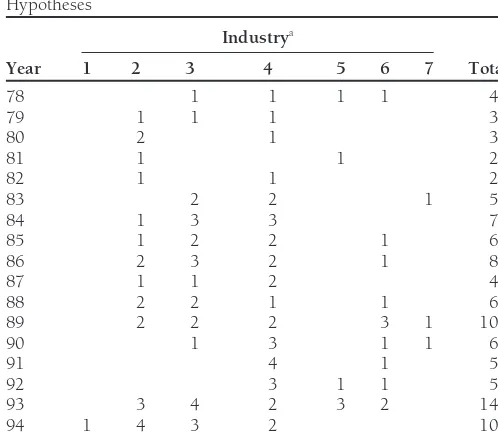
intangi-Table 1. Distribution of Sample Observations _{3. Data is available on total assets, book value of equity,}

and earnings.

Panel A: Sample Observations for Portfolio Tests of Balance Sheet

Hypotheses 4. These observations (for testing the income statement

hypotheses) do not overlap with those used for testing Industrya

the balance sheet hypotheses (which were discussed

Year 1 2 3 4 5 6 7 Total

earlier). By focusing on observations with significant income statement effects but insignificant balance sheet

78 1 3 4

effects, we can more reliably attribute differences in EM

79 2 1 3

80 5 5 ratios to differences in amortization expenses reported

81 1 1 2 _{on the income statement.These criteria result in a}

sam-82 1 1 _{ple of 755 firm-year observations over the 17-year test}

83 2 2

period. There were 241 different firms represented in

84 1 1 1 3

the sample.

85 1 1

86 3 3

SELECTION OF CONTROL OBSERVATIONS. The same 14,683

87 1 3 1 5

firm-year observations described in the balance sheet control

88 3 2 3 2 10

89 2 2 portfolio selection are used.

90 3 2 1 6

91 2 1 1 4

_{Matching Experimental}

92 3 3 1 1 2 10

with Control Observations

93 2 2 2 1 1 8

94 1 4 5 1 2 1 14 _{The same adjustments and matching criteria used for the}

Total 1 18 40 6 9 6 3 83 _{balance sheet portfolio are employed. These criteria result in}

100 matched pairs of adjusted and control observations. Panel

Panel B: Sample Observations for Portfolio Tests of Income Statement

B of Table 1 summarizes the sample distribution by year and

Hypotheses

79 1 1 1 3 _{We first present the results of the portfolio analyses. These}

80 2 1 3 _{results are reported in Tables 2 through 5. We compare mean}

81 1 1 2

(panel A) and median (panel B) values of BM ratios and EM

82 1 1 2

ratios for the experimental, adjusted, and control portfolios.

83 2 2 1 5

84 1 3 3 7 Tables 2 and 4 present the analyses for portfolios with matched

85 1 2 2 1 6 _{observations that are within} ₆_{15% in terms of the three}

86 2 3 2 1 8

control variables (total assets, book value of equity, and

earn-87 1 1 2 4

ings. To provide an indication of the sensitivity of our results

88 2 2 1 1 6

to the choice of the 615% matching criterion, we report

89 2 2 2 3 1 10

90 1 3 1 1 6 corresponding results for observations matched on a610%

91 4 1 5 _{criterion in Tables 3 and 5. The portfolio results are followed}

92 3 1 1 5

by regression analysis results in Table 6. These results serve

93 3 4 2 3 2 14

as a basis for comparison with prior research and for

compari-94 1 4 3 2 10

son with the results of the matched portfolio analysis.

Total 1 21 25 32 6 12 3 100

a_{One-digit SIC codes: 1; mining, oil and gas, and construction; 2; light manufac-}

_{Results of Matched Portfolio Analysis}

turing—food, textile, furniture, printing, and chemical; 3; heavy manufacturing—

rubber, glass, metal, electric, and measuring instrument; 4; transportation, communica- We first present the results of tests of the balance sheet hypoth-tion, and utilities; 5; wholesale and retail trading; 6; finance—banking, brokers, insur- _{eses. These are followed by test results for the income} state-ance, real estate, and investment; 7; personal and business service—hotel, repair, motion

picture, and amusement. ment hypotheses.

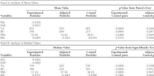
TESTS OF BALANCE SHEET HYPOTHESES. Consistent with the sample selection criteria, the experimental firms exhibit signif-by more than fifty% over the three-year period ending

with the test year. This criterion ensures that the experi- icant amounts of intangible assets as shown in Table 2. The mean (median) proportion of intangible assets to total assets mental firms have stable amounts of amortization

ex-pense for some length of time (i.e., the amortization is 15.78% (18.32%). The results reported in panel A also provide evidence on the efficacy of the matching procedure. expense does not primarily result from recently acquired

(7)

Table 2. Descriptive Statistics of Variables for Experimental, Adjusted and Control Samples for Tests of Balance Sheet Hypotheses

Panel A: Analysis of Mean Values

Mean Value p-Value from Pairedt-Test

Experimental Adjusted Control Experimental-

Adjusted-Variables Portfolio Portfolio Portfolio Control pairs Control pairs

PIA 0.1578

PAE 0.0017

TA 831 705 695 0.0000 0.1406

BE 396 269 275 0.0000 0.2875

EBX 51.00 52.26 52.07 0.2399 0.4909

BM 0.6295 0.4522 0.6195 0.3774 0.0000

Panel B: Analysis of Median Values

Median Value p-Value from Signed-Ranks Test

PIA 0.1832

PAE 0.0000

TA 319 225 230 0.0000 0.1398

BE 184 122 114 0.0000 0.3013

EBX 17.16 17.16 16.23 0.3816 0.4653

BM 0.5571 0.3965 0.5589 0.7966 0.0000

83 matched pairs, control variables are within615%.

Variable definitions: PIA, proportion of reported intangible assets (IA) to total assets (TA); PAE, proportion of amortization expense (AE) to sales; TA, total assets; BE, book value of common equity; EBX, earnings before extraordinary items; BM, book-to-market value ratio5BE/market value of common equity.

of total assets, book value of equity, and earnings across the tent with those reported in Table 2. They suggest that the adjusted and control portfolios. This suggests that it is unlikely earlier conclusions are relatively insensitive to our choice of that observed differences in BM ratios result from differences matching criteria.

in these control variables. We compare BM ratios for the

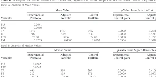
TESTS OF INCOME STATEMENT HYPOTHESES. Sample statistics adjusted and control portfolios to test hypothesis HB1. Both

for testing the two income statement hypotheses are reported the mean and median BM ratios for the adjusted firms are

in Table 4. Consistent with the selection criteria, the experi-less than their corresponding values for the control firms.

mental firms exhibit significant amounts of amortization ex-The parametric pairedt-test and the nonparametric Wilcoxon

pense. The adjusted and control portfolios appear well matched-pairs signed-ranks test indicate that the differences

matched in terms of the control variables. Parametric and in BM ratios are significant at the 0.01 level. These results

nonparametric tests indicate that there are insignificant differ-indicate that the market positively values intangible assets.

ences in total assets, book value of equity, and earnings across To test the second balance sheet hypothesis, we compare

these portfolios. Therefore, it is unlikely that observed differ-BM ratios between the experimental and control firms.

Consis-ences in EM ratios across these portfolios are attributable to tent with the hypothesis, both the mean and median BM

differences in these control variables. ratios for the experimental portfolio are greater than their

Hypothesis HI1 indicates that the adjusted portfolio will corresponding values for the control portfolio. However, the

have a larger EM ratio than the EM ratio for the control differences are not statistically significant. Based on these

re-portfolio. The results reported in panel B show that neither sults, we are unable to reject the null hypothesis that the

the mean nor the median EM ratio for the adjusted firms is market differentially values intangible and tangible assets.

greater than its corresponding value for the control firms. To examine the sensitivity of these results to the matching

Based on this result, we are unable to reject the hypothesis criterion of615% that was used for the control variables, we

that reported amortization expense related to intangible assets repeat the tests by using portfolios that are matched using

is reflected in firms’ equity market values. We compare EM a610% criterion. This stricter criterion enables us to better

ratios for the experimental and control portfolios to test the match the experimental, adjusted, and control portfolios;

second income statement hypothesis. As predicted, the mean however, it results in a smaller number of matched pairs.

and median EM ratios for the experimental portfolio are each Thus, while the power of our tests increases because of the

significantly lower than their corresponding values for the better matching, it is reduced by the smaller number of

(8)

Table 3. Descriptive Statistics of Variables for Experimental, Adjusted and Control Samples for the Tests of Balance Sheet Hypotheses

PIA 0.1478

PAE 0.0018

TA 640 543 542 0.0000 0.9399

BE 310 214 216 0.0000 0.9212

EBX 39.43 40.62 40.24 0.0420 0.9139

BM 0.6947 0.5031 0.6610 0.3176 0.0046

Adjusted-Variables Portfolio Portfolio Portfolio Control Pairs Control Pairs

PIA 0.1373

PAE 0.0000

TA 289 247 248 0.0000 0.8123

BE 153 86 81 0.0000 0.8838

EBX 16.06 16.06 15.96 0.0510 0.8694

BM 0.5894 0.4456 0.6224 0.6893 0.0059

Variable definitions: PIA, proportion of reported intangible assets (IA) to total assets (TA); PAE, proportion of amortization expense (AE) to sales; TA, total assets; BE, book value of common equity; EBX, earnings before extraordinary items; BM, book-to-market value ratio5BE/market value of common equity.

Table 4. Descriptive Statistics of Variables for Experimental, Adjusted and Control Samples for Tests of Income Statement Hypotheses

PIA 0.0641

PAE 0.0066

TA 1547 1467 1462 0.0000 0.2680

BE 609 529 530 0.0000 0.5213

EBX 73.48 80.59 79.08 0.0008 0.3227

EM 0.0733 0.0806 0.0870 0.0364 0.8019

Adjusted-Variables Portfolio Portfolio Portfolio Control pairs Control Pairs

PIA 0.0562

PAE 0.0043

TA 446 399 397 0.0000 0.4159

BE 212 175 172 0.0000 0.6695

EBX 25.13 28.66 26.42 0.0000 0.3194

EM 0.0713 0.0762 0.0776 0.0032 0.8377

(9)

Table 5. Descriptive Statistics of Variables for Experimental, Adjusted and Control Samples for the Tests of Income Statement Hypotheses

PIA 0.0928

PAE 0.0067

TA 2253 2119 2165 0.0007 0.5464

BE 911 776 805 0.0000 0.4218

EBX 117.55 126.52 126.45 0.0998 0.9686

EM 0.0723 0.0783 0.0984 0.0145 0.9559

Adjusted-Variables Portfolio Portfolio Portfolio Control Pairs Control Pairs

PIA 0.0597

PAE 0.0049

TA 554 522 487 0.0002 0.5130

BE 303 184 176 0.0000 0.6368

EBX 35.29 38.11 37.45 0.0001 0.8489

EM 0.0744 0.0801 0.0776 0.0214 0.2070

Variable definitions: PIA, proportion of reported intangible assets (IA) to total assets (TA); PAE, proportion of amortization expense (AE) to sales; TA, total assets; BE, book value of common equity; EBX, earnings before extraordinary items; EM, book-to-market value ratio5EBX/market value of common equity.

market differentially values amortization expense and other resulting from heteroskedasticity. Model 1 is estimated using income statement items. 1,024 firm-year observations with available data over the

pe-Table 5 reports results for matched portfolios based on the riod of study.

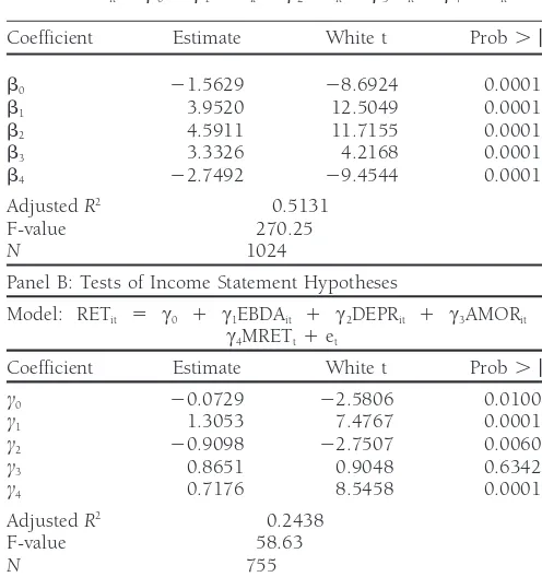
stricter matching criterion of610%. The results are consistent The results of estimating model 1 are reported in panel A with the results reported in Table 4. They indicate that, while of Table 6. They indicate that there is a strong relation between the market differentially values amortization expense and market values of equity and reported book values of assets other income statement items, we are unable to detect the and liabilities, which explain more than 50% of the variation hypothesized negative effect of amortization expense. in market values. The coefficients on the asset variables,b1,

b2, and b3, are all significantly greater than zero while the

Results of Regression Analyses

coefficient on the liabilities variable is significantly negative. The significant positive value for b3 is consistent with the

We first estimate the market value associated with reported

market positively valuing intangible assets. This result is con-intangible assets. We then examine the impact of reported

sistent with Jennings, Robinson, Thompson, and Duvall amortization expense on firms’ market values.

(1996) and McCarthy and Schneider (1995). Consistent with TESTS OF BALANCE SHEET HYPOTHESES. We estimate the

fol-our hypothesis, fol-our results also show that the coefficient on lowing regression model to estimate the relation between

re-IA is less than the coefficients on PPE and ABPI. Thatb3is

ported intangible assets and market value [Eq. (1)]:

less thanb2andb1suggests that the market views the future

MVit5 b01 b1ABPIit1 b2PPEit (1) benefits associated with IA to be more uncertain than the

future benefits associated with PPE or ABPI. This result differs

1 b3IAit1 b4LIABit1 et

from Jennings, Robinson, Thompson, and Duvall (1996) and where MV5 market value of common equity measured at McCarthy and Schneider (1995) who report higher valuations the fiscal year end, ABPI5book value of total assets minus for IA than for PPE and ABPI. One explanation for this differ-property, plant, and equipment and intangible assets, PPE5 ence is that, unlike those studies, our sample is structured to book value of property, plant, and equipment, IA 5 book include firms that have stable intangible assets.10

value of intangible assets, and LIAB5book value of sum of liabilities plus book value of preferred stock.

Each of the above variables is scaled by the beginning-of- 10_{We also estimated model (1) on a year-by-year basis. Inferences from these}

(10)

Table 6. Results of Regression Analysis _{sults also indicate that the coefficient on amortization expense,}

g3, is not significantly related to firm return. This result is

Panel A: Tests of Balance Sheet Hypotheses

consistent with Jennings, Robinson, Thompson, and Duvall (1996), who also find that amortization expense is not signifi-Model:MVit5b01b1ABPIit1b2PPEit1b3IAit1b4LIABit1et

cantly valued by the market. A probable explanation for this

Coefficient Estimate White t Prob.|t| result is that the measure of amortization expense used in financial reports measures the decline in the value of intangible

b0 21.5629 28.6924 0.0001 _{assets with considerable error. The economic value of}

intangi-b1 3.9520 12.5049 0.0001 _{ble assets may decline for some firms but increase for others.}

b2 4.5911 11.7155 0.0001

However, APB Opinion No. 17 requires that intangible assets

b3 3.3326 4.2168 0.0001

be amortized regardless of whether their economic value

in-b4 22.7492 29.4544 0.0001

creases or decreases with the passage of time. This treatment

AdjustedR2 _0.5131

could result in significant measurement error, which may

F-value 270.25

N 1024 explain the insignificant relation between amortization

ex-pense and firm returns observed for our sample firms.

Panel B: Tests of Income Statement Hypotheses

Model: RETit 5 c0 1 c1EBDAit 1 c2DEPRit 1 c3AMORit 1

c4MRETt1et

Summary and Conclusions

Coefficient Estimate White t Prob.|t|

Financial reporting of intangible assets has long been a source

c0 20.0729 22.5806 0.0100

of controversy. Whether reporting of intangible assets and

c1 1.3053 7.4767 0.0001

c2 20.9098 22.7507 0.0060 their related amortization expense provides information that

c3 0.8651 0.9048 0.6342 _{is relevant to market participants’ valuation of firms’ equity}

c4 0.7176 8.5458 0.0001

has been a question of continuing debate among accounting

AdjustedR2 _0.2438

policymakers and academics. This study provides empirical

F-value 58.63

evidence on the major issues of that debate.

N 755

The empirical results based on portfolio analyses indicate that the financial market positively values reported intangible

Variable definitions: RET, annual stock return; EBDA, earnings before extraordinary

items plus depreciation and amortization expenses; DEPR, depreciation expenses of _{assets on the balance sheet but insignificantly regards their} property, plant, and equipment; AMOR, amortization expenses of intangible assets;

amortization expenses on the income statement. The market’s

MRET, equally weighted market return adjusted for dividends payout (EBDA, DEPR,

and AMOR are deflated by beginning market value of comon equity.) _{valuation of a dollar of intangible assets is, however, not}

significantly different from its valuation of other reported bal-ance sheet elements. Therefore, the portfolio tests fail to distin-TESTS OF INCOME STATEMENT HYPOTHESES. We estimate the _{guish intangibles from other balance sheet assets according} following regression model to estimate the relation between _{to the degree and timing of uncertainty in the realization of} reported amortization expense and market value [Eq. (2)]: _{future benefits. Our results also suggest that, although the}

market does not significantly value amortization expense, it RETit5 g01 g1EBDAit1 g2DEPRit (2)

differentially values amortization expense related to intangible

1 g3AMORit1 g4MRETt 1et _{assets and other income statement elements. These results are}

further supported by regression analyses, which indicate that where RET5annual stock return over the fiscal year, EBDA5

there is a positive relation between the book value of intangible earnings before extraordinary items plus depreciation and

assets and the market value of common equity. Moreover, amortization expense, DEPR5depreciation expense on

prop-consistent with the uncertainty hypothesis, the market’s valua-erty, plant, and equipment, AMOR5 amortization expense

tion of a dollar of intangible assets is lower than its valuation on intangible assets, and MRET5equally weighted market

of other reported balance sheet items. With regards to the return adjusted for dividend payout.

income statement hypotheses, the regression analyses show EBDA, DEPR, and AMOR are deflated by beginning of year

that amortization expense is not significantly related to annual market value of common equity. Model 2 is estimated using

stock returns. These findings are consistent with those of the 755 firm-year observations with available data over the period

portfolio analyses. They suggest that either the market does of study.

not view intangible assets as wasting assets or that recorded The results of estimating model 2 are reported in panel B

amortization expense reflects the decline in value of the intan-of Table 6. They indicate that the income statement variables,

gible asset with considerable error. EBDA is significantly positively related to firm return and

The results of our study have several important implica-DEPR is significantly negatively related to firm return. These

tions. First, that intangible assets are positively valued by the results are consistent with theoretical predictions. The market

(11)

Value-Relevance of US versus Non-US GAAP Accounting

Mea-these assets be reported on firms’ balance sheets rather than

sures Using Form 20-F Reconciliations.Journal of Accounting Re-being immediately expensed. Second, that amortization

ex-search31 (1993): 230–264.

pense is not significantly related to stock returns does not

Atiase, R. K.: Predisclosure Information, Firm Capitalization, and

support the current GAAP requirement that reported income _{Security Price Behavior around Earnings Announcements.}_Journal be reduced by the periodic amortization of intangible assets. _{of Accounting Research}_{(1985): 21–35.}

The results of this study suggest that the current GAAP require- _{Chauvin, K. W., and Hirschey, M.: Goodwill, Profitability, and the} ment of periodic amortization of intangible assets be seriously Market Value of the Firm.Journal of Accounting and Public Policy

13 (1994): 159–180.

questioned. One suggestion is that amortization expense be

based on assessed uncertainty in the degree and timing of Egginton, D.: Towards Some Principles for Intangible Asset Account-ing.Accounting and Business Research20 (1990): 193–205.

future benefits expected from each intangible asset. Finally,

Epstein, L. G., and Turnbull, S. M.: Capital Asset Prices and the

that the market value per dollar of intangible assets is less

Temporal Resolution of Uncertainty.Journal of Finance35 (June

than the market value per dollar of tangible assets, and that

1980): 627–643.

the market value associated with each dollar of amortization

Hodgson, A., Okunev, J., and Willett, R.: Accounting for Intangibles:

expense is lower than the market value associated with each

A Theoretical Perspective. Accounting and Business Research 23

dollar of other income statement items, is consistent with _{(1993): 138–150.} relatively greater levels of uncertainty related to intangible

Jennings, R., Robinson, J., Thompson II, R. B., and Duvall, L.: The

assets and amortization expense. These results support the _{Relation between Accounting Goodwill Numbers and Equity} Val-criticism of financial statements’ failure to reflect differential ues. Journal of Business Finance and Accounting23 (1996): 513–

533.

levels of uncertainty across their different elements. They

sug-gest that accounting reports would be more informative to Johnson, J. D., and Tearney, M. G.: Goodwill—An Eternal Contro-versy.The CPA Journal53 (April 1993): 58–62.

decision makers if they include information on differences in

Lang, M.: Time-Varying Stock Price Response to Earnings Induced

uncertainty related to future economic benefits (costs) across

by Uncertainty about the Time Series Process of Earnings.Journal their different elements.

of Accounting Research29 (Autumn 1991): 229–257.

McCarthy, M. G., and Schneider, D. K.: Market Perception of

Good-We thank John Wild, Douglas Schneider, and the anonymous reviewer for

will: Some Empirical Evidence.Accounting and Business Research valuable comments. Won Choi acknowledges financial support from Dongguk

26 (1995): 69–81.

University, Sung Kwon from the School of Business at Rutgers University,

Rabe, J. G., and Reilly, R. F.: Valuing Health Care Intangible Assets.

and Gerald Lobo from the George E. Bennett Research Center and the Office

National Public Accountant41 (March 1996): 14–43.

of the Vice President of Research and Computing at Syracuse University.

Reilly, R. F.: The Valuation of Intangible Assets. National Public Accountant41 (July 1996): 26–40.

References

_{Robichek, A. A., and Myers, S. C.: Valuation of the Firm: Effects of}

American Institute of Certified Public Accountants, Accounting Prin- Uncertainty in a Market Context. Journal of Finance 21 (June ciple Board. 1970. APB Opinion No.17—Intangible Assets. New 1966): 215–227.

York, NY: AICPA. _{Rubinstein, M. E.: A Mean-Variance Synthesis of Corporate Financial}