Analysis of dierence approximations to a singularly perturbed
two-point boundary value problem on an adaptively
generated grid
Y. Qiu1, D.M. Sloan∗
Department of Mathematics, University of Strathclyde Glasgow G1 1XH, Scotland, UK
Received 4 April 1998; received in revised form 14 May 1998
Abstract
Over the last few years there has been a signicant growth in the use of adaptive grid methods for the numerical solution of dierential equations with steep solutions. Little has been done, however, on the error analysis of adaptive methods. In this paper, we present an analysis for an upwind nite dierence solution of a singular perturbation problem on a grid that is generated adaptively by equidistributing a monitor function based on the exact solution. It is shown that the discrete solutions converge uniformly with respect to the perturbation parameter, epsilon. This epsilon-uniform convergence is illustrated by numerical computations. c1999 Elsevier Science B.V. All rights reserved.
1. Introduction
There has been a great deal of work done recently on the use of adaptive nite-dierence methods for steady and unsteady solutions of partial dierential equations. An overview of some of this work may be obtained, for example, in Refs. [3, 6, 7, 14, 24]. A review of the literature on adaptive methods will show that signicant progress is being made on the construction of methods, but contributions to the analysis of adaptive methods are virtually nonexistent. The aim here is to make a contribution in this area by analysing an upwind nite-dierence solution of a simple model dierential equation on a grid that approximates an adaptively generated grid. In particular, we consider the model problem
(Lu)(x)≡ −u′′
(x)−p(x)u′
(x) = 0; x∈(0;1);
u(0) = 0; u(1) = 1; (1.1)
∗
Corresponding author. E-mail: [email protected].
where is a constant satisfying 0¡ 61. It is assumed furthermore that p∈C2[0;1] and that there are constants a; b and P∗ such that
p(x)¿P∗¿ a ¿0 ∀x∈[0;1] (1.2)
and
b= max
06x61{p(x);|p
′
(x)|}: (1.3)
For ≪1 the model problem has a boundary layer of thickness O() near the boundary x= 0. It is well known that a centred or upwind dierence scheme on a uniform mesh will not give a satisfactory numerical solution to a problem such as (1.1) if ≪1. To obtain a reliable numerical solution in a computationally ecient manner it is essential to use a mesh that concentrates nodes in regions where the solution gradient is large [4]. Ideally, the mesh should be adapted to the features of the solution using an adaptive grid generation technique. This approach is now widely used for numerical solution of dierential equations with steep, continuous solutions. A common theme in adaptive nite dierence methods is the concept of equidistribution, which seeks to distribute some nonnegative monitor function evenly over the domain of the problem. This monitor function is normally some measure of computational error or solution variation, but the ideal choice of monitor function is still an open question (see, for example, [2, 7, 13, 20, 24] and references therein). The paper by Mulholland et al. [13] shows that extremely accurate computational solutions of singular perturbation problems have been obtained on adapted meshes. Here we give some insight into the nature of the convergence of these solutions by considering the approximate solution of (1.1) using a rst-order upwind method on an adaptively graded mesh. Numerical computations show that the pointwise errors are bounded by a quantity that tends to zero at a rate that is independent of . The numerical method, comprising the dierence scheme and the mesh, is convergent uniformly with respect to the singular perturbation parameter, .
Discrete methods whose solutions converge independently of are said to be -uniform. In par-ticular, a method of solving (1.1) is -uniform convergent on the mesh
N≡ {xj:xj=xj−1+hj; j= 1;2; : : : ; N: x0= 0; xN = 1} (1.4)
if there exists a positive integer N0, and positive numbers C and q, with N0; C and q independent of N and , such that for N¿N0,
max
06j6N|u(xj)−uj|6CN
−q
: (1.5)
Here u is the solution of (1.1), {uj}Nj=0 is the numerical approximation to u, and q is the -uniform rate of convergence. If a method is -uniform, mesh renement causes the error bound to decrease in a manner that is independent of the perturbation parameter.
demonstrated -uniform convergence on the Shishkin mesh (see also the texts [12, 17], and the review [16]). Stynes and Roos [19] consider an upwind scheme for an inhomogeneous form of (1.1) on a Shishkin mesh. Their interesting paper establishes that convergence is -uniform of ‘almost’ rst order, with
|u(xj)−uj|6CN
−1lnN; ∀j= 0;1; : : : ; N:
A hybrid scheme is also presented in [19] that is -uniform convergent of ‘almost’ second order. The rst attempt to solve singular perturbation problems on an exponentially graded mesh was that presented by Bakhvalov [1] in 1969. The name Bakhvalov is now used to describe a mesh that is exponentially graded within the boundary layer and equidistant outside the layer. Vulanovic [22] has investigated uniform convergence on Bakhvalov-type meshes in which the exponential grad-ing function is approximated by a more convenient function. Vulanovic [23] has also considered Bakhvalov-type meshes for singularly perturbed boundary value problems with turning points (inte-rior layers). Finally, on this theme, the work by Gartland [5] on exponentially graded meshes is of interest. He shows how to construct schemes that have arbitrarily high uniform order of convergence. For a problem on [0;1] with a boundary layer atx= 0, Gartland has an inner region [0; x∗] in which the mesh is exponentially graded, an outer region [x′
;1] in which the grid is uniform and a transition region [x∗; x′
] in which the mesh is geometrically graded.
The objective of this paper is to show that adaptivity may be used to generate a mesh for which
-uniform convergence is readily achieved. The mesh is produced by equidistributing a monitor function that is based on the exact solution of (1.1). The mesh is an approximation to that which is produced by a fully adaptive scheme based on the equidistribution of a computed approximation to the monitor function. For the monitor function that we have selected in this work, the equidistribution process gives rise to an exponentially graded mesh. This mesh is related to the Bakhvalov-type meshes presented in [1, 22], within the boundary layer region. However, the grid generation by means of equidistribution is a novel feature that adds signicantly to the potential of this mode of analysis. Adaptive methods are also eective in approximating solutions of problems with interior layers [13], so the analysis presented here might give a possible route to the treatment of a wider class of near-singular problems.
In Section 2 we present the dierence scheme — including the choice of grid — and we discuss some properties of the solution of (1.1) that are required in the analysis. Section 3 describes the analysis of the-uniform convergence for the standard rst-order upwind scheme on a logarithmically graded mesh that is generated by equidistribution. A similar analysis is outlined in Section 4 for a second-order upwind scheme. Section 5 deals with discretisations in a computational space that is related to physical space by means of an adaptively generated logarithmic map: it is shown that -uniform convergence is readily obtained using discretisation on an even grid in this mapped space. Concluding comments are given in Section 6, and illustrative numerical results are presented throughout the paper.
It should be emphasised that the analysis presented in this paper deals only with semi-discretisation of the adaptive method. We use the term semi-discretisation to indicate that the exact solution of (1.1) is used in the equidistribution principle to generate the mesh, and the solution {uj}Nj=0 is then computed on this generated mesh. A fully discretised scheme is one in which a discrete approximation of the equidistribution principle is combined with the nite dierence equation to give a nonlinear algebraic system for the set of unknowns {xj; uj}N
−1
the convergence behaviour of the semi-discretised system and thereby gain some insight into the convergence of the fully discretised system.
2. Dierence scheme and properties of solution of (1.1)
2.1. Dierence scheme
To obtain an appreciation of the nature of an uneven mesh that may be appropriate for the compu-tational solution of (1.1) we initially consider the simplied model given by setting the coecientp
equal to unity. For this model, the exact solution is
u(x) =1−e
−x=
1−e−1=: (2.1)
Here, u is a strictly monotonic increasing function of x and we may construct a mesh by equidis-tributing the monitor function M(u(x); x) = du=dx over the domain [0;1] (see, for example [7]). This gives rise to a mapping, x=x(), relating the computational coordinate ∈[0;1] to the physical coordinate x∈[0;1], dened by
Z x
0
M(u(s); s) ds= Z 1
0
M(u(s); s) ds: (2.2)
With M = du=dx this equation yields
=u(x) (2.3)
and
x=−ln (1−Lˆ ); (2.4)
where ˆL = 1−exp (−1=). To construct a mesh of the form (1.4) we obtain the nodes {xj}Nj=0 in physical space corresponding to the evenly distributed nodes j =j=N for j = 0;1; : : : ; N in
computational space. This identication gives
xj=−ln (1−Lj=Nˆ ); j= 0;1; : : : ; N; (2.5)
and we note that
hj=xj−xj−1; j= 1;2; : : : ; N: (2.6)
The upwind dierence approximation to (1.1) that we wish to analyse on a mesh such as that dened by (2.5) is
(L
u)(j)≡ −(D+D−u)(j)−pj(D+u)(j) = 0; j= 1;2; : : : ; N −1;
(u)(0) = 0; (u)(N) = 1;
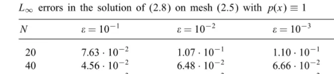
Table 1
L∞ errors in the solution of (2.8) on mesh (2.5) withp(x)≡1
N = 10−1 = 10−2 = 10−3 = 10−4
20 7:63·10−2
1:07·10−1
1:10·10−1
1:11·10−1
40 4:56·10−2 6
:48·10−2 6
:66·10−2 6
:67·10−2 80 2:62·10−2 3:75·10−2 3:85·10−2 3:86·10−2 160 1:46·10−2
2:11·10−2
2:16·10−2
2:17·10−2
where pj=p(xj) and u is the mesh function with (u)(j) denoting the approximation, uj, to u(xj).
The operators D+; D− and D+D− are the familiar divided dierence operators, given by
(D+u)(j) =
uj+1−uj hj+1
; (D−u)(j) =
uj−uj−1
hj ;
(D+D−u)(j) =
(D+u)(j)−(D−u)(j)
1
2(hj+1−hj−1)
:
Scheme (2.7) is conveniently expressed as
−Cjuj−1+Ajuj−Bjuj+1= 0; j= 1;2; : : : ; N −1;
u0= 0; uN = 1;
(2.8)
where
Aj=
2 hjhj+1
+ pj
hj+1
;
Bj=
2 hj+1(hj+hj+1)
+ pj
hj+1
;
Cj=
2 hj(hj+hj+1)
:
Note that
Aj¿0; Bj¿0; Cj¿0 and Aj=Bj+Cj (2.9)
for j= 1;2; : : : ; N −1.
If (1.1) with p(x)≡1 is solved on mesh (2.5) by means of scheme (2.8) the numerical results show that the method is -uniform of order 1, provided is suciently small. Table 1 shows the maximum pointwise (L∞) error at various values of N and .
It is readily seen that for N¿40 and for the range of values used, the error behaviour satises an inequality of form (1.5) with q= 1.
A weakness in mesh (2.5) that we have constructed for the simplied version of (1.1) is that the nodes {xj}N
−1
j=1 are contained in a narrow region close to x= 0. For example, with N = 20 and
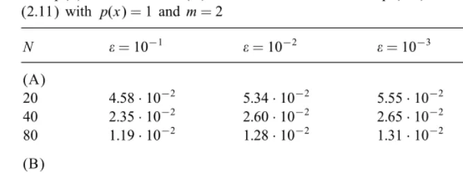
Table 2
(A)L∞errors in the solution of Eq. (2.8) coupled with the equidistribution equation (2.2),
withp(x) = 1 andm= 2. (B)L∞errors in solution of Eq. (2.8) on a mesh generated by
(2.11) withp(x) = 1 andm= 2
N = 10−1
= 10−2
= 10−3
= 10−4 (A)
20 4:58·10−2
5:34·10−2
5:55·10−2
5:71·10−2 40 2:35·10−2 2:60·10−2 2:65·10−2 2:69·10−2 80 1:19·10−2
1:28·10−2
1:31·10−2
1:33·10−2
(B)
20 4:58·10−2 5:29·10−2 5:34·10−2 5:34·10−2 40 2:37·10−2
2:62·10−2
2:63·10−2
2:63·10−2
80 1:20·10−2
1:29·10−2
1:29·10−2
1:29·10−2
a mesh that is more convenient — both theoretically and computationally — may be obtained from (2.2) if the monitor function, M, is given by
M(u(x); x) =
du
dx 1=m
; m= 2;3; : : : : (2.10)
If (2.2) denes a mapping x=x(), then
dx
dM(u(x()); x()) =K= constant:
With M as in (2.10) and u given by (2.1), the map from [0;1] to [0;1] is
x=−mln(1−L˜ ); (2.11)
where ˜L= 1−exp(−1=m). A mesh is now generated by assigning :=j=j=N for j= 0;1; : : : ; N.
On this mesh, the computed solution of the constant coecient form of (1.1) is again found to be
-uniform of order 1.
At this preliminary stage it is of interest to compare the semi-discretised and the fully discretised adaptive strategies in terms of convergence behaviour. One should recall that we hope to use the former to gain some insight into the latter. As shown in [7], the equidistribution equation (2.2) is approximated by
Mj+1=2(xj+1−xj) =Mj−1=2(xj−xj−1); j= 1;2; : : : ; N −1; (2.12)
where Mj+1=2 denotes an approximation to M at 12(xj +xj+1). The approximation is obtained by solving (2.8) and (2.12) simultaneously for {xj; uj}N
−1
j=1 . Table 2(A) shows the maximum pointwise error in the computed solution of (1.1) with p(x) = 1, based on the fully discretised adaptive method with monitor function (du=dx)1=2. Table 2(B) shows the corresponding results obtained by solving the dierence equations (2.8) on the mesh given by (2.11).
The results in Tables 2(A) and (B) show an error behaviour that satises inequality (1.5) with
We infer from the computational results with p(x)≡1 that an obvious scheme for the variable coecient problem (1.1) is an adaptive one based on the monitor function (2.10). To simplify the treatment of the variable coecient case we construct the monitor function (2.10) in terms of the exact solution of (1.1) with p(x) set to the constant lower bound, a. This yields the mesh
xj=−
m
a ln(1−Lj=N); j= 0;1; : : : ; N (2.13)
based on the monotonic map
x=−m
a ln(1−L); (2.14)
where L= 1−exp(−a=m). If the variation of p is small on the interval [0;1], the nodes (2.13) are likely to be close to those given by simultaneous solution of (2.8) and (2.12) with M= (du=dx)1=m.
The convergence behaviour of the semi-discretised scheme on the mesh (2.13) is likely to be close to that of the fully discretised adaptive scheme. Henceforth we shall be concerned with the approximate solution of (1.1) by means of scheme (2.8) on the mesh (2.13).
2.2. Properties of solution of (1.1)
The exact solution of (1.1) is
u(x) =G(x)
In the subsequent analysis we shall require bounds on the local truncation errors of the dierence scheme. Here we obtain bounds on those derivatives of u that occur in the local truncation errors.
For 61 we may write G(1)¿=c1, where c1=b=(1−e
The second derivative of u is
u′′
and this may be written as
|u′′′
(x)|¡ c3
−3e−ax= ∀x∈[0;1]: (2.19)
The key results of this section are conveniently summarised as
06u(x)61; |u(k)(x)|6c
k
−ke−ax= (k= 1;2;3); (2.20)
∀x∈[0;1], where ck(k= 1;2;3) are constants that are independent of .
3. Analysis of scheme (2.8) and (2.13)
3.1. Local truncation error
The local truncation error of (2.8) at node xj in (2.13) is
j= (Lu)(j)−(Lu)(xj); (3.1)
from which we obtain the bound
|j|¡ Z xj+1
xj−1
|u′′′
(s)|ds+b Z xj+1
xj−1
|u′′
(s)|ds:
If we invoke the derivative bounds given in (2.20) this may be simplied to
|j|¡ c Z xj+1
xj−1
|u′′
(s)|ds; (3.3)
where c is constant that is independent of . We shall use the symbol c to denote a generic constant throughout the analysis that follows.
To initiate the construction of an appropriate bound for the local truncation error we replace|u′′
(s)|
by the bound given in (2.20) to obtain
|j|¡ c
−2Z xj+1
xj−1
e−ax=dx
=c−1Z j+1
j−1
(1−L)m−1d; using (2:14):
If the range of integration is bisected we obtain
|j|¡2c
−1Z j
j−1
(1−L)m−1d
= 2c
N(1−L
)m−1
; where ∈(j−1; j):
Now,
1−L ¡ 1−Lj−1= (1−Lj) +L=N;
and
L=N ¡1−Lj=N for j= 1;2; : : : ; N −1:
Hence, 1−L ¡ 2(1−Lj), and it follows that
|j|¡ c
N(1−Lj)
m−1¡ c
N(1−Lj);
which yields
|j|¡ c
Ne
−axj=m
; j= 1;2; : : : ; N −1: (3.4)
We nd that (3.4) is acceptable for j = 1;2; : : : ; N −2, but, owing to the proximity of xN−1 to
x0, the subsequent error analysis dictates that we require a stronger result for the bound on |N−1|. To this end, suppose is the smallest positive integer that satises 10−
6≪1, and select m such that m¿+ 2. Now write
|N−1|¡
c
N(1−LN−1)· 1
(1−LN−1)
and ensure that N is chosen such that the term [·] does not exceed unity. The required condition is
The required bounds on the local truncation errors are given by (3.5) and
|j|¡ c
Ne
−axj=m
; j= 1;2; : : : ; N −2: (3.6)
3.2. Bound on maximum point-wise error
If the dierence scheme (2.7) is combined with expression (3.1) for the local truncation error, we obtain the equation
(Le)(j) =j; j= 1;2; : : : ; N −1; (3.7)
where e is the mesh function of nodal errors, with e(j) =u(xj)−uj. Eq. (3.7) is row j of the linear
algebraic system
in which L∈R(N−1)×(N−1) is a tridiagonal matrix with elements given by {−C
j; Aj;−Bj}, as dened
in (2.8), and = [1; 2; : : : ; N−1]T. In the subsequent analysis we make use of properties of L that
are given in the following lemma. The analysis is akin to that used be Kellogg and Tsan for an evenly spaced mesh [9].
Lemma 3.1. System (Lu)(j) =fj; with u(0) and u(N) specied; has a solution. If (Lu)(j)¡
(Lv)(j); 16j6N−1; and if u(0)¡ (0); u(N)¡ v(N); then u(j)¡ v(j); 16j6N−1.
Proof. The matrix L is diagonally dominant and has non-positive o diagonal terms, as shown
in (2.9). Hence the matrix is an irreducible M matrix [21], and so it has a positive inverse. Hence the solution u(j);16j6N−1 exists and u(j)¡ v(j);16j6N.
The following two lemmas are also used in the subsequent analysis.
Lemma 3.2.
(i) hj¡ m
a ; j= 1;2; : : : ; N −1;
(ii) hN= O(1):
Proof. For j= 1;2; : : : ; N −1,
hj=−
m
a [ln(1−Lj)−ln(1−Lj−1)]
=mL
aN ·
1
1−Lj; where j∈(j−1; i):
Similarly,
hj+1=
mL
aN ·
1
1−Lj+1; j+1∈(j; j+1);
and since 1 1−Lj ¡
1 1−Lj+1;
it follows that
hj¡ hj+1; j= 1;2; : : : ; N −1:
Also,
1 1−Lj ¡
1 1−Lj
;
so
hj¡ mL
aN ·
1 1−Lj=N =
m
a ·
1
N=L−j¡
m
a ·
1
Thus, hN−1¡ m=a, and since hj¡ hj+1 for j= 1;2; : : : ; N−2, result (i) follows. Finally,
PN
j=1hj= 1
and hj= O(); j= 1;2; : : : ; N −1, imply that hN = O(1) for 0¡ ≪1.
Lemma 3.3. The mesh function; e; satises the inequality
(Le)(j)¡ c
Proof. Noting that xj may be written as Pjk=1hk, Eq. (3.6) is written alternatively as
|j|¡
The result for j=N −1 is obtained similarly.
We are now able to proceed with the construction of a bound on the solution of the error equation (3.7) using an approach related to that adopted in [19]. It is convenient to introduce the quantities
and it is readily shown that
Noting that Sj+1=Sj=rj+1, we may write
For notational convenience we denote (L
S)(j) by L{Sj} and obtain the inequality
If (3.11) is used in the statement of Lemma 3.3 the resulting inequality is
L{ej}¡ c
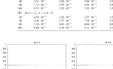
Table 3
L∞ errors of solution of equation (2.8) on mesh (2.13)
N = 10−1
= 10−2
= 10−3
= 10−4
(A) p(x) = 1; a= 1 2; m= 6
20 6:21·10−2 1:01·10−1 1:02·10−1 1:02·10−1 40 3:31·10−2
5:56·10−2
5:56·10−2
5:56·10−2
80 1:71·10−2
2:95·10−2
2:95·10−2
2:95·10−2 160 8:71·10−3 1:52·10−2 1:52·10−2 1:52·10−2 (B) p(x) = 1
1+x; a= 1 3; m= 6 20 6:28·10−2
1:26·10−1
1:27·10−1
1:27·10−1 40 3:36·10−2 7:37·10−2 7:38·10−2 7:38·10−2 80 1:74·10−2 4:03·10−2 4:04·10−2 4:05·10−2 160 8:86·10−3
2:10·10−2
2:11·10−2
2:11·10−2
Fig. 1. Meshes given by (2.13) withN= 40 and = 0:001. The left and right displays correspond tom= 2 and m= 6, respectively.
computed solution of (1.1), with p(x) = 1 and p(x) = 1=(1 +x), by means of (2.8) on mesh (2.13). The results illustrate an -uniform convergence of order 1.
The value m= 6 was used in the computation of the results in Table 3 in order to satisfy the constraint m¿v+ 2 for 10−v
4. An -uniform scheme of second order
The preceding sections have dealt with the attainment of -uniform convergence by virtue of a specially adapted mesh. An alternative approach is to use a dierence scheme that reects the sin-gularly perturbed nature of the dierential operator: such nite-dierence operators are referred to as tted nite-dierence operators (see, for example, [12, p. 15]). In this section we consider the use of the tted dierence operator proposed by Il’in [8] on the mesh (2.13). We shall demon-strate — theoretically and computationally — that this scheme is second-order -uniform convergent. In fully discretised adaptive computations, a possible strategy would be to generate the adaptive mesh by combining the equidistribution principle with a simple (coecients easily computed) rst-order upwind scheme to produce {xj; uj}N
−1
j=1 . The higher-order tted scheme could then be applied as a post-processor on the generated grid.
We consider (L(2)
u)(j) = 0, given by
−qj coth (qj)(D+D−u)(j)−pj(D0u)(j) = 0; j= 1;2; : : : ; N −1;
(u)(0) = 0; (u)(N) = 1:
(4.1)
Here, D0 is the dierence operator
(D0u)(j) =
uj+1−uj−1
hj+hj+1
and qj= pjhj
2 :
This scheme was considered by Kellogg and Tsan [9] for the approximate solution of a singular perturbation problem on an evenly spaced mesh.
At node xj, the local truncation error of (4.1) as an approximation of (1.1) is
j=−[qjcoth (qj)−1](D+D−){u(xj)}
−[(D+D−){u(xj)} −u ′′
(xj)]−pj[(D0){u(xj)} −u
′
(xj)];
which enables us to write, in the obvious notation,
|j|6A+B+pjC; j= 1;2; : : : ; N −1: (4.2)
A form of this bound analogous to the bounds (3.5) and (3.6) that were used in the error analysis of scheme (2.8) is given by Eqs. (A.9) and (A.10) in the appendix. For convenience, we display the bounds here as
|N−1|¡
c N2e
−axN
−1=m; (4.3)
|j|¡ c
N2e
−axj=m; j= 1;2; : : : ; N −2: (4.4)
For the error analysis of scheme (4.1) we also require conditions that are analogous to inequalities (3.11). To this end we note that (4.1) may be written as (2.8), where Aj, Bj and Cj are now given
by
Aj=
2qjzj hjhj+1
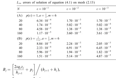
Table 4
L∞ errors of solution of equation (4.1) on mesh (2.13)
N = 10−1
= 10−2
= 10−3
= 10−4
(A) p(x) = 1; a= 1 2; m= 6
20 6:34·10−4 1:70·10−3 1:70·10−3 1:70·10−3 40 1:74·10−4
5:02·10−4
5:02·10−4
5:02·10−4
80 4:58·10−5
1:38·10−4
1:38·10−4
1:38·10−4 160 1:17·10−5 3:60·10−5 3:61·10−5 3:61·10−5 (B) p(x) = 1
1+x; a= 1 3; m= 6 20 8:84·10−4 2
:24·10−3 2
:05·10−3 2
:03·10−3 40 2:33·10−4 6:91·10−4 6:45·10−4 6:40·10−4 80 5:96·10−5
1:94·10−4
1:82·10−4
1:81·10−4
160 1:51·10−5 5
:14·10−5 4
:87·10−5 4
:83·10−5
Bj= "
2qjzj hj+1
+pj #,
(hj+1+hj);
Cj= "
2qjzj hj
−pj #,
(hj+1+hj):
Here zj denotes coth (qj) and it is clear that
Aj¿0; Bj¿0; Cj¿0 and Aj=Bj+Cj for j= 1;2; : : : ; N −1:
We now introduce the quantities {Sj}Nj=0 as dened by (3.9). In the appendix we prove (see (A.12) and (A.13)) that
L(2)
{Sj}¿
c
Sj; j= 1;2; : : : ; N −2; (4.5)
L(2)
{SN−1}¿ cSN−1: (4.6)
From the error equation, L(2)
e=, it is readily shown using (4.3)–(4.6) and the analysis leading
to (3.12) that for scheme (4.1) the pointwise error bound is
|ej|¡ c
N2; j= 0;1; : : : ; N: (4.7)
This establishes that scheme (4.1) with mesh (2.13) is second-order -uniform convergent. Table 4 shows the maximum pointwise error in the computed solution of (1.1), with p(x) = 1 and p(x) = 1=(1 +x), by means of (4.1) on mesh (2.13). The results illustrate an -uniform convergence of order 2.
5. Discretisation in computational space
a monotonic map x=x(). Rather than use the map to generate the mesh {xj}Nj=0 as in (2.13), we use it to express the dierential equation in terms of the independent variable . The transformed equation is then discretised on an even grid in the coordinate . In practical computations, the map
x=x() will be generated by an adaptive algorithm, and the process of solving the transformed equation will then be regarded as an accurate post-processing step. The ecacy of this approach is demonstrated by the pseudospectral post-processing work of Mulholland et al. [13]. The aim of this section is to show that the discrete solutions converge at a rate that matches the formal order of accuracy of the post-processing scheme, provided the map x=x() is suciently smooth. In the work presented here, we make the analysis tractable by using the map (2.14) that arises from the equidistribution of the exact solution of (1.1). If the map is specied, and v() denotes u(x()), we may transform (1.1) to
v+ (p(x()))x−x=x)v= 0;
v(0) = 0; v(1) = 1; (5.1)
where the subscript denotes dierentiation with respect to . It is of interest to compare the discretisations on a graded mesh described in the preceding sections with that which arises when (5.1) is discretised on an even grid in the computational coordinate. If we use the same logarithmic map (2.14), Eq. (5.1) is readily transformed to
v+
. We now give an outline of the convergence analysis of scheme (5.3): the approach is analogous to that described fully in Section 3.
The local truncation error of (5.3) at node j is
j=
the second and fourth derivatives of v in terms that involve derivatives of u with respect to x and derivatives of x with respect to . Map (2.14) yields the essential derivatives of x as
The second and fourth derivatives of v are, respectively,
and these may be expressed completely in terms of derivatives of u by means of (5.5). To obtain bounds on |j| we have to extend the bounds given by (2.20) to include d4u=dx4. To achieve this,
we extend the denition of b given in (1.3) to
b= max
06x61{p(x);|p
′
(x)|;|p′′
(x)|}:
Making use of this, the analysis leading to (2.19) is readily extended to give
|u(4)(x)|¡|u′ If the extended (2.20) is written as
|u(k)(x)|6c
k
−k
(1−L)m; (k = 1;2;3;4) (5.7)
with related to x by (2.14), it is readily shown, using (5.5)–(5.7), that
Eq. (5.8) leads to a bound on the local truncation error in (5.4) that may be written as
|j|6
To obtain a bound on the pointwise error we make use of Lemma 3.1. It is readily shown that the tridiagonal system associated with scheme (5.3) is an irreducible M matrix. Furthermore, if this (N −1)×(N −1) matrix is denoted by L and ˆS ≡[1; 2; : : : ; N−1]T, then
(LSˆ)(j) =−w(j)L
1−Lj
where d is a positive lower bound on w()L, ∈(0;1). The constant d is independent of the parameter . If Sj= 2−j; j= 0;1; : : : ; N, and S= [S1; S2; : : : ; SN−1]T then
(LS)(j)¿ d; j= 1;2; : : : ; N −1: (5.10)
This inequality is the analogue of condition (3.11) that arose in the analysis of the graded grid case. As in the earlier case, we combine this with the error equation
(Le)(j) =j; j= 1;2; : : : ; N −1; (5.11)
to obtain the required error bound. In the obvious notation we see that
L{ej}=j6|j|¡ Ch ¡
Ch
d L{Sj}=L
ChS j d
; j= 1;2; : : : ; N −1:
Since 0 =e0¡ Ch S0=d and 0 =eN¡ Ch SN=d, it follows from Lemma 3.1 that
ej¡ Ch Sj
d ; j= 0;1; : : : ; N:
Since ej may be replaced by −ej, we see that
|ej|¡ Ch Sj
d 6ch; j= 0;1; : : : ; N; (5.12)
where c is a generic constant that is independent of and N. Eq. (5.12) establishes that the scheme (5.3) — constructed by means of the map (2.14) — is rst-order -uniform convergent.
It is clear from the above that the analysis is more tractable when the discretisation is eected on an even grid in the transformed space. If the map is chosen properly the solution is well behaved in this space and this leads to the simpler treatment. On the evenly spaced grid in the coordinate it is fairly straightforward to construct schemes that are -uniform of order q, where q ¿1. For example, if g() denotes w()L=(1−L), the scheme
1 1 + (h=2)g(j)
·vj+1−2vj+vj−1
h2 +g(i)
vj+1−vj
h = 0; j= 1;2; : : : ; N −1; v0= 0; vN = 1;
(5.13)
is readily shown to be a second-order approximation of (5.2) provided hg(j)¡2 forj=1;2; : : : ; N−
1. Furthermore, the dierence operator dened by (5.13) is an irreducible M matrix that satises inequality (5.10). An analysis similar to that given above readily establishes that
|ej|¡ ch2; j= 0;1; : : : ; N; (5.14)
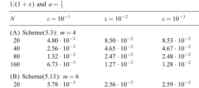
if m¿6, where c is independent of and N. Hence (5.13) is second-order -uniform convergent. Table 5 shows the maximum pointwise error in the computed solution of (1.1) withp(x) = 1=(1 +x), by means of (5.3) and (5.13) on mesh (2.13) with a=1
3 and m= 4 in (A) and m= 6 in (B). The results below conrm that schemes (5.3) and (5.13) are -uniform convergent of orders 1 and 2, respectively. As in previous cases,-uniform convergence is achieved in practical computation, even if we remove the restriction on m that we required in the analysis.
Table 5
L∞ errors of solution of (1.1) by schemes (5.3) and (5.13) on mesh (2.13) withp(x) =
1=(1 +x) and a=1 3
N = 10−1 = 10−2 = 10−3 = 10−4
(A) Scheme(5.3): m= 4 20 4:80·10−2
8:50·10−2
8:53·10−2
8:53·10−2
40 2:56·10−2
4:65·10−2
4:67·10−2
4:67·10−2 80 1:32·10−2 2:47·10−2 2:48·10−2 2:48·10−2 160 6:73·10−3 1:27·10−2 1:28·10−2 1:28·10−2 (B) Scheme(5.13): m= 6
20 5:78·10−3 2:56·10−2 2:59·10−2 2:59·10−2 40 1:62·10−3
8:46·10−3
8:62·10−3
8:62·10−3
80 4:32·10−4
2:49·10−3
2:54·10−3
2:54·10−3 160 1:11·10−4 6:79·10−4 6:94·10−4 6:95·10−4
equation and the reconditioned problem is then solved on the coordinate using a pseudospectral discretisation. The computed solutions exhibit spectral accuracy.
6. Concluding remarks
We have presented a convergence analysis for the nite dierence solution of a singularly perturbed two-point boundary value problem without turning points. The solution is obtained on a mesh that arises from the exact equidistribution of the monitor function dened by (2.10). The analysis shows that if the mesh is generated adaptively, it is possible to obtain dierence solutions that converge uniformly with respect to the perturbation parameter.
The work presented here gives some insight into the nature of the convergence of adaptive dif-ference schemes as the mesh is rened. It is, however, limited in several respects: for example, the monitor function should ideally be bounded below by a constant that is positive rather than zero. This limitation has been partially removed in a subsequent paper that deals with the solution of (1.1) on a mesh that is based on an arc-length monitor function [15]. Work is also being carried out on extending the arc-length treatment to deal with more general two-point boundary value problems than those represented by (1.1). The ultimate goal, of course, is to gain insight into the nature of the convergence of schemes in which the mesh and the physical solution are generated together using a fully adaptive scheme.
Appendix A
A.1. Local truncation error
Referring to (4.2), it is readily seen that
where c again denotes a generic constant and u denotes the exact solution of (1.1). Since qj=pjhj=26chj=, we obtain, using (2.20),
To proceed with the analysis j=N −1 we introduce a convenient lemma.
Lemma A.1.
Proof. From (2.20) we see that
and it follows that
From the expression for u′′′
(x) following (2.18) we obtain
|u′′′
and the statement of the lemma is now a consequence of (i) and (ii). Lemma A.1 permits us to recast (A.4) in the form
B6ch2N−1|u
′′′
(xN−1)|;
and this combines with (A.3) to give the bound
B6c h2j|u′′′
From within the proof of Lemma 3.2 we extract the bound
Map (2.13) gives the alternative formulation
hj¡ c
Ne
axj=m;
and if this is combined with the bound on |u′′′
(xj)| given in (2.20) we are able to write (A.7) as
|j|¡ c
N2e
−axj=
;
where =m=(m−2). We shall assume m ¿2 so that is positive and bounded. Since 6m we may write the local truncation error bound in the relaxed form
|j|¡ c
N2e
−axj=m
(A.8)
that proves to be more convenient for the subsequent error analysis.
Result (A.8) is analogous to the bound given by (3.4) for the scheme considered in Section 3 of the paper. In a manner similar to that used in the consideration of (3.5) and (3.6) we obtain the bounds
|N−1|¡
c N2e
−axN−1=m; (A.9)
|j|¡ c
N2e
−axj=m
; j= 1;2; : : : ; N −2: (A.10)
A.2. Bound on maximum point-wise error
Here we establish inequalities (4.5) and (4.6) that are required in the error analysis of scheme (4.1). Using (4.1), we see that for j= 1;2; : : : ; N −1,
(hj+1+hj)(L
(2)
S)(j) =−pj(Sj+1−Sj−1) +
2qjzj hj
(Sj−Sj−1)−
2qjzj hj+1
(Sj+1−Sj)
=−pj(Sj+1−Sj−1)−2dqjzjSj+ 2dqjzjSj+1;
on making use of (3.10). Further applications of (3.10), together with the relation
Sj+1=Sj=rj+1=
Sj
1 + dhj+1=
;
enable us to write
(hj+1+hj)(L(2)S)(j) =FjSj; (A.11)
where
Fj= pj =d+hj+1
hj+1+hj+ d
hjhj+1(1−zj)
:
Hence,
Fj¿ pj =d+hj+1
[hj+1+hj+hj+1G(j)];
where G() =(1−coth()). As in the analysis of scheme (2.8) leading to inequalities (3.11), we consider the cases j= 1;2; : : : ; N −2 and j=N −1 separately.
For j = 1;2; : : : ; N −2 we know from Lemma 3.2 that dhj+1¡ , and since G() is strictly
monotonic increasing for ¿0 we have G(j)¿−1. These conditions enable us to write
Fj¿ pjdhj
2 ¿ adhj
2 :
Furthermore, an analysis akin to that used in Lemma 3.2 readily shows that
hj¿16(hj+1+hj);
and it follows that
Fj¿ ad
12(hj+1+hj):
This combines with (A.11) to show that
L(2)
{Sj}¿
c
Sj; j= 1;2; : : : ; N −2: (A.12)
For j=N −1, we may show, using a mean value argument, that
hN−1¿
mL
3a ; provided N ¡e
a=m+ 2:
This givesN−1=ahN−1=m ¿L
3, and it follows from the monotonicity ofGthatG(N−1)¿ G(L=3)=
−c ¿−1.
Since dhN−1¿ we may write
FN−1¿
a
2hN
(hN +hN−1)
1− chN hN +hN−1
¿ c(hN +hN−1):
Finally, this combines with (A.11) to show that
L(2)
{SN−1}¿ cSN−1: (A.13)
References
[1] A.S. Bakhvalov, On the optimization of methods for solving boundary value problems with boundary layers, Zh. Vychisl. Mat. i Mat. Fis. 9 (1969) 841– 859 (in Russian).
[2] G.F. Carey, H.T. Dinh, Grading functions and mesh redistribution, SIAM J. Numer. Anal. 22 (1985) 1028 –1040. [3] E.A. Dor, L.O’C. Drury, Simple adaptive grids for 1-D initial value problems, J. Comput. Phys. 69 (1987) 175 –195. [4] F.W. Dorr, The numerical solution of singular perturbations of boundary value problems, SIAM J. Numer. Anal.
[5] E.C. Gartland, Graded-mesh dierence schemes for singularly perturbed two-point boundary value problems, Math. Comput. 51 (1988) 631– 657.
[6] W. Huang, Y. Ren, R.D. Russell, Moving mesh partial dierential equations (MMPDEs) based on the equidistribution principle, SIAM J. Numer. Anal. 31 (1994) 709 –730.
[7] W.-Z. Huang, D.M. Sloan, A simple adaptive grid method in two dimensions, SIAM J. Sci. Comput. 15 (1994) 776 –797.
[8] A.M. Il’in, Dierencing scheme for a dierential equation with a small parameter aecting the highest derivative, Math. Notes 6 (1969) 596 – 602.
[9] R.B. Kellogg, A. Tsan, Analysis of some dierence approximations for a singular perturbation problem without turning points, Math. Comput. 32 (1978) 1025 –1039.
[10] J.A. Mackenzie, Uniform convergence analysis of an upwind nite-dierence approximation of a convection– diusion boundary value problem on an adaptive grid, IMA J. Numer. Anal. (accepted).
[11] J.J.H. Miller, E. O’Riordan, G.I. Shishkin, On piecewise-uniform meshes for upwind- and central-dierence operators for solving singularly perturbed problems, IMA J. Numer. Anal. 15 (1995) 89–99.
[12] J.J.H. Miller, E. O’Riordan, G.I. Shishkin, Fitted Numerical Methods for Singular Perturbation Problems, World Scientic, Singapore, 1996.
[13] L.S. Mulholland, W.-Z. Huang, D.M. Sloan, Pseudospectral solution of near-singular problems using numerical coordinate transformations based on adaptivity, SIAM J. Sci. Comput., 19 (1998) 1261–1289.
[14] L.S. Mulholland, Y. Qiu, D.M. Sloan, Solution of evolutionary partial dierential equations using adaptive nite dierences with pseudospectral postprocessing, J. Comput. Phys. 131 (1997) 280 –298.
[15] Y. Qiu, D.M. Sloan, Tao Tang, Convergence analysis of an adaptive nite dierence method for a singular perturbation problem, submitted for publication.
[16] H.-G. Roos, Layer-adapted grids for singular perturbation problems, MATH-NM-03-1997, Technische Universitat Dresden Report.
[17] H.-G. Roos, M. Stynes, L. Tobiska, Numerical Methods for Singularly Perturbed Dierential Equations, Springer, Berlin, 1996.
[18] G.I. Shishkin, Grid approximation of singularly perturbed elliptic and parabolic equations, Second Doctoral Thesis, Keldysh Institute, Moscow, 1990 (in Russian).
[19] M. Stynes, H.-G. Roos, The midpoint upwind scheme, Appl. Numer. Math., 23 (1997) 361–374.
[20] J.F. Thompson, Z.U.A. Warsi, C.W. Mastin, Numerical Grid Generation, North-Holland, New York, 1985. [21] R.S. Varga, Matrix iterative analysis, Prentice-Hall, Englewood Clis, NJ, 1962.
[22] R. Vulanovic, Mesh construction for discretization of singularly perturbed boundary value problems, Doctoral dissertation, University of Novi Sad, 1986.
[23] R. Vulanovic, Non-equidistant generalizations of the Gushchin–Shennikov scheme, ZAMM 67 (1987) 625– 632. [24] A.B. White, On selection of equidistribution meshes for two-point boundary value problems, SIAM J. Numer. Anal.