Minimum variance quadratic unbiased estimators as a tool
to identify compound normal distributions
Jean-Daniel Rolle∗
HEC-Management Studies, University of Geneva, CH-1211 Geneva, Switzerland, HEG-Haute Ecole de Gestion, CH-1700, Fribourg, Switzerland
Received 31 August 1997; received in revised form 7 September 1998
Abstract
We derive the minimum variance quadratic unbiased estimator (MIVQUE) of the variance of the components of a random vector having a compound normal distribution (CND). We show that the MIVQUE converges in probability to a random variable whose distribution is essentially the mixing distribution characterising the CND. This fact is very important, because the MIVQUE allows us to make out the signature of a particular CND, and notably allows us to check if an hypothesis of normality for multivariate observations y1; : : : ; yM is plausible. c1999 Elsevier Science B.V. All rights reserved.
Keywords:Normal linear regression; Compound normal distributions; Quadratic estimation; Error components model
1. Introduction
Suppose that our data are individual N-variate observations ym, m= 1; : : : ; M, that are (multivari-ate) measures of a phenomenon. The measurements were performed under changing conditions. A reasonable model for these observations (or measures) is the linear systemym=+Um, whereis an
N×1 location vector, and, conditional on a random scale parameter,Umis Gaussian:Um∼N(0; ). This means that the ym have a compound normal distribution. We examine here how we can learn something about the distribution of , and enlarge the problem by assuming that we have known covariate information on the location parameter, so that =(X) =X. Zellner [13] describes cases where the scale mixtures of normal prove useful in practice. He notes that one may look at the multivariate realisations ym of Y, m= 1; : : : ; M, as being generated by a measuring instrument. The variability of the instrument, represented by a scale factor for the covariance matrix, has an unknown
∗E-mail: [email protected].
value within a run and is known to vary over the M runs. Rolle [10] used this model to study ag-gregated multivariate measures performed under changing circumstances, when data are produced in a network setting.
It is well known that compound normal distributions with high kurtosis will produce outliers. We propose here a procedure to detect departures from the multivariate normal distribution which is not directly related to the question of detection of multivariate outliers. The latter has known important developments during the last decade. Rousseeuw and Van Zomeren [12] note that usual techniques mask outlier detection, and propose to replace in the Mahalanobis distance the arithmetic mean of the data set and the sample covariance matrix by estimators with high breakdown point. More precisely, they use the minimum volume ellipsoid estimator introduced by Rousseeuw [11]. Their technique immediately applies to identication of leverage points in regression. In this context, the authors propose a plot of standardized least median of squares residuals versus robust distances; this plot proves very useful to classify observations. Cook and Hawkins [3] showed that a method based on minimum volume ellipsoid estimators may indicate too many outliers, and that the approximate algorithm used for their computation may be instable. Rocke and Woodru [7] give insights into why the problem of outlier detection is so dicult, specially in high dimensionalities, and a method incorporating an algorithm proposed by Atkinson [1]. Atkinson’s [2] forward search is based on robust estimators: the least median of squares estimators for regression and the minimum volume ellipsoid for multivariate outliers. Our aim here is not to unmask outliers, but to nd what kind of random mechanism produced the outliers in a well-dened parametric setting.
2. The necessary tools
To provide a procedure able to detect departures from the multivariate normal distribution, we analyze the behavior of quadratic estimators. First of all, let us recall a few denitions needed in the sequel. Let be a N×1 vector and a N×N symmetric matrix. A N×1 random vector Z
Gaussian distribution, and H is a distribution function for the nonnegative random scale parame-ter . From this denition, if Z∼CN(; ; H), then equivalently one has that, conditional on ,
Z∼N(; ). The distribution of is a mixing distribution, and the class of CND is obtained by varying this distribution [6]. IfH is degenerated on= 1, that is if takes the value 1 with probabil-ity 1, thenf(z) = N(z;; ), that is Z is Gaussian. IfZ has a CND, then its characteristic function is of the form cZ(t) = eit
′
H(t
′
t) for some function H (depending on H, as the notation suggests). Provided that relevant moments exist, one has E(Z) = and Cov(Z) = −2′
H(0)=EH()=V, say. For example, if Z is Gaussian with f(z) = N(z;; ), then H(s) = exp(−s=2), and V=. Moreover, if Z= (Z1; : : : ; ZN)′ has nite fourth moments, then the marginal distributions Zj all have zero skewness and the same kurtosis 3(′′
3. The model and the main results
We consider here the linear regression model
y=X+U; (2)
where U is a N×1 vector of disturbances, X is a N×K known matrix, not necessarily of full rank, and is a K×1 vector of regression coecients. We assume that U in (2) is such that
U∼CN(0; 2I;
H). Let the covariance matrix of the error vector be V= Cov(U) =2I. A special case of this model was considered by Zellner [13], where U was assumed to follow a multivariate Student-t distribution. More general forms can be assumed for V without changing the qualitative results. Notably, the conclusions are the same if V has the structure of a covariance matrix from the error components model, a model well known by econometricians working on p-way classied data. Here we will
1. Find the minimum variance unbiased estimator ˆ2 of 2 among the quadratics y′
Ay with A¡0,
i.e. we will seek the nonnegative MIVQUE. We show that this estimator is
ˆ
2= 1
N−rXy
′
(I −XX+)y; (3)
where X+ is the Moore–Penrose inverse of X, and rX denotes the rank of X. Note that this estimator does not depend on any particular (mixing) distribution of and hence on any particular CND (in that sense, it is a uniform MIVQUE).
2. Show that ˆ2 converges in probability (and hence in distribution) to2=E
H(), where EH denotes mathematical expectation.
We can draw two conclusions from 2. First, ˆ2 converges in probability to a random variable, and hence is inconsistent, unless U is Gaussian — in that case, is degenerated on 1. Thus, the MIVQUE cannot be used per se. This shows that the minimum variance criterion can be a rather poor criterion for chosing estimators. Second, and more promisingly, we have that for reasonably large N, the distribution function of ˆ2 is essentially H. Hence, if we have a set of i.i.d. N-variate observations yi; i= 1; : : : ; M, of mean X, that we suspect to come from a heavy-tailed distribu-tion, we can model yi∼CN(X; 2I; H). An analysis of the (empirical) distribution of the indepen-dent ˆ2i =y′
iMXyi=(N −rX), where MX =I −XX+, will provide much information about how the
yi were generated. In particular, concentration of the ˆ2i around a single point indicates normality. As ˆ2 has approximatively (for large N) the distribution of 2=E
H(), we propose the following process: (i) We assume that we have i.i.d. realizations y1; : : : ; yM of y. (ii) We compute ˆ21; : : : ;ˆ
2 M and their mean a= (Pˆ2i)=M. (iii) We compute t1= ˆ21=a; : : : ; tM= ˆ2M=a. The t1; : : : ; tM approximate realizations of =EH(). (iv) We analyze the distribution of the ti (thanks to usual tools such as boxplots, histograms, etc.) to detect potential non-Gaussian features. Next, as H= varH(=EH()), the sample variance s2
t of the ti will provide an estimate of H. Note that H= 0 in the Gaussian case, and H¿0 otherwise. The higher the H, the larger the departure from normality. Various simulations showed that this technique works very well. Although more formal procedures can be developed to exploit this nding, we shall here content ourselves with a brief description. Let 1 be a
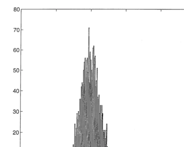
Fig. 1. We simulated M= 2000 N-variate (N= 100) Gaussian realizations yi= 1+Ui, where 1 is a N×1 vector of ones, and Ui∼N(0;4I), i= 1; : : : ; M. In such a case, we have simply X= 1. Then we computed the quadratics ˆ
2i=y′iMXyi=(N−1). The M values ti were obtained by dividing the ˆ2i by their mean. Fig. 1 displays the resulting histogram of the ti and suggest concentration around 1.
d.f., that isH=2
5. The histograms of the ti for the three cases appear in Figs. 1–3. As the theoretical ndings predict, they indicate concentration around one point for (a), 80% concentration around 1
4, and 20% around 4 for (b), and the shape of the 2
5 divided by its mean, 5, for (c). We tookN= 100 for this simulation, but even for N with magnitude 20 or 30, non-Gaussian features can be detected. Of course, the smaller the N, the more diuse this information. The corresponding approximations
s2
t of H may be read in Table 1. More formal analysis such as approximate normality tests, or density estimation, may be applied to this data generating mechanism, and are the object of current research.
4. Proof of the statements
We rst prove 1. above, i.e. we show that (3) is the MIVQUE. Using Li Gang’s result from Fang and Anderson [4], one can show that if Z∼CN(; ; H), and Z′AZ is such that A= 0, then
Var(Z′
AZ) =H(trAV)2+ 2(H + 1)trAVAV : (4)
Next, since U∼CN(0; 2I;
H), then y=X+U∼CN(X; 2I; H). Let y
′
Ay be a potential es-timator for 2. Nonnegativity and unbiasedness (E(y′
Ay) =2) imply AX= 0, as one can show easily. Hence A=AX= 0 and, since E(Z′
AZ) = trAV, we have that E(y′
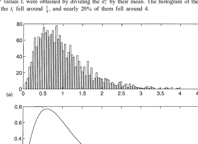
Fig. 2. Simulation ofM= 2000N-variate (N= 100) contaminated realizationsyi= 1+Ui, whereUi is 0.8N (0,I)+0.2N (0,16I). TheM valuesti were obtained by dividing the ˆ2i by their mean. The histogram of theti suggests contamination: nearly 80% of theti fell around 14, and nearly 20% of them fell around 4.
Fig. 3. Simulation of M= 2000N-variate (N= 100) realizationsyi= 1+Ui, where Ui∼N(0; I), conditional on ∼25.
Table 1
P)]−2. Therefore we can equivalently minimize on the open set P the dif-ferentiable function (P) = tr (MXP
converges in probability to 2. More-over, 2= −2′
(0)2, and −2′
(0) =EH(), by a moment generating property of the characteristic function. That is, ˆ2 converges in probability to 2=E
the components of U are exchangeable (but not independent). The law of large numbers for such sequences allows the limit to be a random variable. This is what happens here.
References
[1] A.C. Atkinson, Stalagtite plots and robust estimation for the detection of multivariate outliers, in: S. Morgenthaler, E. Ronchetti, W. Stahel, Data Analysis and Robustness (Eds.), Birkhaueser, Basel, 1993.
[2] A.C. Atkinson, Fast very robust methods for detection of multiple outliers, J. Amer. Statist. Assoc. 428 (1994) 1329 –1339.
[3] R.D. Cook, D.M. Hawkins, Comments on Unmasking multivariate outliers and leverage points, by P.J. Rousseeuw and B.C. Van Zomeren, J. Amer. Statist. Assoc. 85 (1990) 640– 644.
[4] K.T. Fang, T.W. Anderson, Statistical Inference in Elliptically Contoured and Related Distributions, Allerton Press, New York, 1990.
[5] J.R. Magnus, H. Neudecker, Matrix Dierential Calculus with Applications in Statistics and Econometrics, Wiley, New York, 1988.
[6] R.J. Muirhead, Aspects of Multivariate Statistical Theory, Wiley, New York, 1982.
[7] D.M. Rocke, D.L. Woodru, Identication of outliers in multivariate data, J. Amer. Statist. Assoc. 428 (1996) 1329 –1339.
[8] J.D. Rolle, Best nonnegative invariant partially orthogonal quadratic estimation in normal regression, J. Amer. Statist. Assoc. 428 (1994) 1378–1385.
[9] J.D. Rolle, Optimization of functions of matrices with application in statistics and econometrics, Linear Algebra Appl. 234 (1996) 261–275.
[10] J.D. Rolle, Aggregated multivariate measures performed under changing circumstances, The Indian J. Statist.: Sankhya, Ser. A, 60 (2) (1998) 232–248.
[11] P.J. Rousseeuw, Multivariate estimation with high breakdown point, in: W. Grossman et al. (Eds.), Mathematical Statistics and Applications, vol. B, Reidel, Dordrecht, 1985.
[12] P.J. Rousseeuw, B.C. Van Zomeren, Unmasking multivariate outliers and leverage points, J. Amer. Statist. Assoc. 441 (1990) 633– 639.