www.elsevier.nl/locate/cam
Adaptive nite element–boundary element solution of
boundary value problems
O. Steinbach
Universitat Stuttgart, Mathematisches Institut A, Pfaenwaldring 57, D 70569 Stuttgart, Germany
Received 21 September 1998
Abstract
An adaptive nite element–boundary element algorithm is proposed to compute an approximate solution of a given boundary value problem. The convergence inH1() is controlled by a boundary element based a-posteriori error estimator
from which an adaptive renement strategy is derived. Corresponding error estimates are given based on appropriate boundary element error estimates in negative Sobolev norms. c1999 Elsevier Science B.V. All rights reserved.
Keywords:Boundary element; Finite element; Adaptivity
1. Introduction
For the solution of a homogeneous Dirichlet boundary value problem,
Lu(x) = 0 for x∈⊂Rn (n= 2;3); u(x) =g(x) for x∈ :=@ (1.1)
with an elliptic second order partial dierential operator L we consider a boundary element method,
where an approximate solution of Eq. (1.1) is described by a representation formula involving an approximate boundary element solution. The (linear) interpolation of this solution denes a nite
element function within the bounded domain . Using again the representation formula for the
solution and its partial derivatives we are able to control the error of this nite element–boundary element solution and we can dene some adaptive strategy to construct a solution having an almost
minimal error in H1() for a xed boundary element solution. Besides an accurate computation of
a nite dimensional solution of Eq. (1.1) we can use the nal triangulation of our approach as an initial mesh in nite element computations for more complicated problems as in Eq. (1.1), i.e., in the case of partial dierential operators with non-constant coecients, or even as a boundary element a-posteriori error estimator in nite element computations. Note that the consideration of Dirichlet boundary conditions in Eq. (1.1) does not restrict the applicability of our method. For mixed boundary
value problems one may use any boundary element method to compute approximate solutions for the unknown Cauchy data. Then one can apply the method proposed in this paper directly. Moreover, the generalisation to inhomogeneous partial dierential equations in Eq. (1.1) will be straightforward. The use of boundary element methods is the numerical solution of boundary integral equations which are equivalent to the original boundary value problem, for an introduction, see e.g. [9]. In Section 2 we describe a direct boundary integral approach which is discretized by a Galerkin method. Note that also qualocation or collocation schemes may be applied. For the solution of mixed boundary value problems using boundary integral equations and boundary elements, see e.g. [2,13]. If an approximate boundary element solution is determined, the solution of the original
boundary value problem can be computed inside pointwise with a high accuracy due to available
error estimates in negative Sobolev norms [6]. However, in many applications one is interested in a nite dimensional solution of the original problem to be used in a postprocessing such as visualisation, computation of functionals including the solution or in nonlinear solution processes. In Section 3 we give an adaptive strategy to compute such a solution, where we use a boundary element based a-posteriori error estimator to dene an appropriate renement of the mesh. Note that after computing the boundary element solution once, no further linear systems have to be solved. Some considerations of the numerical amount of work are given in Section 4. Section 5 is devoted to the numerical analysis of our method, i.e., to give corresponding error estimates. A numerical example in Section 6 underlines the advantage of the proposed method even in a comparison with an adaptive nite element computation.
2. Boundary element methods
If a fundamental solution U∗(x; y) of the partial dierential operator L in Eq. (1.1) is given, the
solution of the boundary value problem (1.1) can be described by the representation formula
u(x) =
x→ , Eq. (2.1) gives the boundary integral equation
(Vt)(x) =1 2g(x) +
Z
g(y)T∗
(x; y) dsy= : f(x) for x∈ (2.2)
with the single layer potential operator
(Vt)(x) =
For a family of boundary triangulations h we consider trial spaces
Zh:= span{’k} N k=1⊂H
−1=2( ) (2.4)
of discontinuous splines of polynomial degree , e.g. of piecewise constant trial functions (= 0).
Then the Galerkin variational formulation of Eq. (2.2) is to nd th∈Zh such that
Note that we may solve Eq. (2.5) for an adaptive rened family of triangulations h and
corre-sponding trial spaces Zh up to some required accuracy. After a nal boundary element solution th is
computed, replacing in Eq. (2.1) t by th, an approximate solution of Eq. (1.1) is given by
uh(x) =
In the next section we will describe a nite dimensional approximation of Eq. (2.6) by using a nite
element interpolation with respect to an adaptive triangulation of .
3. An adaptive postprocessing algorithm
For the bounded domain we consider a family of regular triangulations
H=
N
X
k=1
k (3.1)
with an initial or coarse triangulation H0 and M nodal points xk. With respect to (3.1) we dene
the usual nite element trial space
WH = span{ k}Mk=1 ⊂H
1() (3.2)
of piecewise linear hat functions. Using Eq. (3.2) we dene an approximate nite element solution of Eq. (1.1) by
with coecients given by the approximate representation formulae (2.6) and (2.7),
˜
uk=uh(xk) for k= 1; : : : ; M: (3.4)
Note that ˜uH is the linear interpolant for uh inWH. To controll the error of the approximate solution
(3.3) and to get a renement strategy we dene an approximate nite element error locally as
ke˜HkH1(k):=kuh(x)−u˜H(x)kH1(k) for k = 1; : : : ; N (3.5)
and rene all nite elements k where
ke˜HkH1(k)¿· max
l=1;:::; N ke˜HkH
1(l) (3.6)
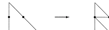
is satised with some appropriate renement parameter . To avoid hanging nodes and to get a
Fig. 1. Renement strategy for three hanging nodes.
Fig. 2. Renement strategies for two hanging nodes.
Fig. 3. Renement strategies for one hanging node.
Note that we have to stop this renement strategy when some level of accuracy is reached which
depends clearly on the accuracy of the boundary element solution th.
Using the local error estimators (3.5) we are able to dene a global error estimator as
ke˜HkH1()=
N
X
k=1
ke˜Hk2H1(
k)
!1=2
: (3.7)
4. Numerical complexity
The numerical complexity of the proposed algorithm consists of the part to solve the Galerkin boundary element formulation (2.5), the computation of the nite element–boundary element solution (3.3) by computing (3.4) via the representation formulae (2.6), (2.7) and the application of the local error estimators (3.5).
Since the stiness matrix of the discrete single layer potential V in Eq. (2.5) is in general dense,
the Galerkin discretization of Eq. (2.5) as well as an iterative solution of the discrete linear
sys-tem will require O(N2) operations. Note that this can be reduced when using fast acceleration
techniques such as panel clustering [4]. The computation of the nite element–boundary element
so-lution requires O(MN ) operations. Note that one has to compute all nodal values only once since
representation formula (2.6) to compute the local error estimator (3.5) will cost O(NN ) operations. Therefore, the complexity of our nite element–boundary element algorithm can be estimated as
O(N (N +M+N)): (4.1)
An optimal nite element computation will cost O(M[logM]) operations in computing the solution
and O(N) to get an error estimator. In our numerical example we will see that we can choose N
to be signicantly smaller than M andN, respectively. Hence we claim that the proposed method
is comparable to standard nite element methods when considering partial dierential equations with constant coecients. Moreover, due to available error estimates in negative Sobolev norms, the boundary element based error estimator may provide more accurate results as it will be seen from the numerical example.
5. Error estimates
In this section we provide all required error estimates for the boundary element solution th of
Eq. (2.5) as well as error estimates according to Eqs. (3.3) and (3.5). First we note that in Zh there
holds the approximation property [8], i.e., for 6s6+ 1 and ¡1
h of the Galerkin formulation (2.5) is uniquely determined
[15] and satises the error estimate [5,6,9]
kt−thkH( )6c·hs−· ktkHs( ) (5.2)
ift∈Hs( ) and −2−66s6+1; ¡1
2 (n=2); 60 (n=3). Hence we get the maximal error
reduction ofh2+3 when measuring the error in theH−2−( ) norm, if the solutiontis regular enough.
Note that the local bounds in Eq. (5.2) may dier when using interpolated boundary conditions gh
instead of g in the Galerkin formulation (2.5). Now it is straightforward that for x∈ far enough
from the boundary we get the error estimate
|u(x)−uh(x)|6
one can use other techniques to compute the solution uh(x) with high accuracy [10,12]. In a similar
manner as in Eq. (2.6) we can compute the partial derivatives in x∈ by
@
providing similar error estimates as given in Eq. (5.3).
Theorem 5.1. Let u∈H(); 62; be the solution of Eq.(1:1). For the nite element–boundary
element solution u˜H given by Eq. (3:3) there hold the pointwise error estimate for x∈k
|u(x)−u˜H(x)|6c·H
and the local error estimates
ku−u˜HkL2(k)6c·Hk· |u|H(k)+c·H
Proof. Using the pointwise error estimate (5.3) we get
|u(x)−u˜H(x)|6|uh(x)−u˜H(x)|+|u(x)−uh(x)|
uH is the linear interpolant of uh we can apply standard error estimates [1, Chapter 4] to derive Eq.
(5.5). Note that kuh kH(
k) can be bounded by kukH(k) due to denition (2.6). Taking the
square and integrating over k gives Eq. (5.6). Using corresponding error estimates for 3u˜H we
can derive Eq. (5.7).
From Eq. (5.7) we get directly the global estimate
ku−u˜HkH1(
As in the proof of Theorem 5.1 we get also
| ku−u˜HkH1(
which provides that the error estimator (3.5) is equivalent to the error if h is suciently small.
6. Numerical example
As numerical example we consider for n= 2 the Dirichlet boundary value problem
u(x) = 0 for x∈; u(x) =g(x) for x∈ ; (6.1)
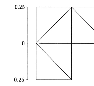
where is the L shaped domain as sketched in Fig. 4.
In Eq. (6.1) the given Dirichlet data are taken in such a way that the exact solution of the boundary value problem (6.1) is given in polar coordinates by
u(x) =u(r; ’) =r23·sin2’
3 : (6.2)
First we solve the Galerkin boundary integral formulation (2.5) starting from an initial triangulation
of N = 8 boundary elements. Using an a-posteriori error estimator as described in [11] we get a
Fig. 4. L shaped domain and initial triangulation. Table 1
H1() error of the nite–boundary element solution
Estimated Exact
M N Absolute Relative Absolute Relative
8 6 1:66−1 3:04−1 1:66−1 3:05−1
17 20 1:14−1 2:08−1 1:14−1 2:08−1 28 40 8:26−2 1:51−1 8:27−2 1:51−1 49 76 5:96−2 1:09−1 5:96−2 1:09−1 73 122 4:52−2 8:26−2 4:53−2 8:27−2 131 230 3:34−2 6:09−2 3:34−2 6:11−2 189 338 2:72−2 4:97−2 2:73−2 4:98−2 350 646 1:97−2 3:60−2 1:97−2 3:59−2 596 1116 1:49−2 2:72−2 1:49−2 2:72−2 1095 2086 1:09−2 2:00−2 1:10−2 2:01−2 2003 3868 8:09−3 1:48−2 8:21−3 1:50−2
are solved by a conjugate gradient method using a preconditioner as proposed in [14] which is well suited for the adaptive renement case. In the example described here it was sucient to stop the
boundary element computation after using N = 86 boundary elements yielding a L2 error of
kt−thkL2( )= 2:47×10−1:
Using the Galerkin boundary element solution th we dene the nite element–boundary element
solution (3.3) rst on the initial domain triangulation as shown in Fig. 4 and then on the rened
triangulation when applying the renement criteria (3.6) with = 0:3. In Table 1 we give both the
estimated error (3.7) and the exact error ku−uHkH1() using the exact solution given by Eq. (6.2)
for all levels of mesh renement.
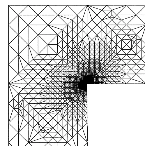
For an assessment of our results we rst use a nite element computation on the nest nite
element–boundary element triangulation shown in Fig. 5 with M= 2003 nodes getting an error of
ku−uhkH1()= 8:02×10−3;
ku−uhkH1() kukH1()
Fig. 5. FEM=BEM triangulation with 2003 nodes.
Hence, the nite element–boundary element solution we computed is closed to the nite element solution minimizing the energy norm | · |H1() in WH.
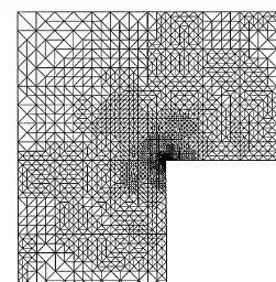
Using the results given in [7] we can compare our results with an adaptive nite element compu-tation based on an error estimator given in [3]. For the nal triangulation as shown in Fig. 6 with
M= 1990 nodes and N= 3904 volume elements the approximate nite element solution has an
error of
ku−uhkH1()= 1:22×10−2;
ku−uhkH1() kukH1()
= 2:24×10−2:
Summarizing the numerical results we conclude that the nite element–boundary element method proposed gives a triangulation providing some slightly better error results than an adaptive nite element computation. Note that the nite element–boundary element solution was computed just with 86 boundary elements only, and that the computation of the coecients is a postprocessing without solving any linear system.
Fig. 6. FEM triangulation with 1990 nodes.
Acknowledgements
Part of this work was done while the author was a Postdoctoral Research Associate at the Institute for Scientic Computation (ISC), Texas A&M University, College Station. The nancial support of the ISC is gratefully acknowledged. Special thanks are due to S. Tomov (ISC) for performing all the nite element computations described in this paper.
References
[1] S.C. Brenner, L.R. Scott, The Mathematical Theory of Finite Elements, Springer, New York, 1994.
[2] M. Costabel, E.P. Stephan, Boundary integral equations for mixed boundary value problems in polygonal domains and Galerkin approximation, in: Mathematical Models and Methods in Mechanics, Banach Center Publications, vol. 15, Warsaw, 1985, pp. 175 –251.
[3] K. Eriksson, C. Johnson, An adaptive nite element method for linear elliptic problems, Math. Comput. 50 (1988) 361–382.
[4] W. Hackbusch, Z.P. Nowak, On the fast matrix multiplication in the boundary element method by panel clustering, Numer. Math. 54 (1989) 463–491.
[5] G.C. Hsiao, W.L. Wendland, A nite element method for some integral equations of the rst kind, J. Math. Anal. Appl. 58 (1977) 449–481.
[6] G.C. Hsiao, W.L. Wendland, The Aubin–Nitsche lemma for integral equations, J. Integral Equations 3 (1981) 299– 315.
[7] R. Lazarov, J. Pasciak, S. Tomov, Multilevel grid renement for elliptic problems based on a posteriori error analysis, Technical Report, ISC, Texas A&M University, 1998.
[9] A. Schatz, V. Thomee, W.L. Wendland, Mathematical Theory of Finite and Boundary Element Methods, Birkhauser, Basel, 1990.
[10] H. Schulz, C. Schwab, W.L. Wendland, The computation of potentials near and on the boundary by an extraction technique for boundary element methods, Comput. Methods Appl. Mech. Eng. 157 (1998) 225–238.
[11] H. Schulz, O. Steinbach, A new posteriori error estimator in adaptive direct boundary element methods. The Dirichlet problem, submitted, 1998.
[12] C. Schwab, W.L. Wendland, On the extraction technique in boundary integral equations, Math. Comput. 68 (1999) 91–122.
[13] O. Steinbach, Fast solution techniques for the symmetric boundary element method in linear elasticity, Comput. Meth. Appl. Mech. Eng. 157 (1998) 185–191.
[14] O. Steinbach, W.L. Wendland, The construction of some ecient preconditioners in the boundary element method, Adv. Comput. Math. 9 (1998) 191–216.