Think Bayes by Allen B. Downey
Copyright © 2013 Allen B. Downey. All rights reserved.
Printed in the United States of America.
Published by O’Reilly Media, Inc., 1005 Gravenstein Highway North, Sebastopol, CA 95472.
O’Reilly books may be purchased for educational, business, or sales promotional use. Online editions are also available for most titles (http://my.safaribooksonline.com). For more information, contact our corporate/ institutional sales department: 800-998-9938 or [email protected].
Editors: Mike Loukides and Ann Spencer Production Editor: Melanie Yarbrough Proofreader: Jasmine Kwityn Indexer: Allen Downey
Cover Designer: Randy Comer Interior Designer: David Futato Illustrator: Rebecca Demarest
September 2013: First Edition
Revision History for the First Edition:
2013-09-10: First release
See http://oreilly.com/catalog/errata.csp?isbn=9781449370787 for release details.
Nutshell Handbook, the Nutshell Handbook logo, and the O’Reilly logo are registered trademarks of O’Reilly Media, Inc. Think Bayes, the cover image of a red striped mullet, and related trade dress are trademarks of O’Reilly Media, Inc.
Many of the designations used by manufacturers and sellers to distinguish their products are claimed as trademarks. Where those designations appear in this book, and O’Reilly Media, Inc., was aware of a trade‐ mark claim, the designations have been printed in caps or initial caps.
While every precaution has been taken in the preparation of this book, the publisher and authors assume no responsibility for errors or omissions, or for damages resulting from the use of the information contained herein.
ISBN: 978-1-449-37078-7
Table of Contents
Preface. . . ix
1. Bayes’s Theorem. . . 1
Conditional probability 1
Conjoint probability 2
The cookie problem 3
Bayes’s theorem 3
The diachronic interpretation 5
The M&M problem 6
The Monty Hall problem 7
Discussion 9
2. Computational Statistics. . . 11
Distributions 11
The cookie problem 12
The Bayesian framework 13
The Monty Hall problem 14
Encapsulating the framework 15
The M&M problem 16
Discussion 17
Exercises 18
3. Estimation. . . 19
The dice problem 19
The locomotive problem 20
What about that prior? 22
An alternative prior 23
Credible intervals 25
Cumulative distribution functions 26
The belly button data 175
Predictive distributions 179
Joint posterior 182
Coverage 184
Discussion 185
Index. . . 187
Preface
My theory, which is mine
The premise of this book, and the other books in the Think X series, is that if you know how to program, you can use that skill to learn other topics.
Most books on Bayesian statistics use mathematical notation and present ideas in terms of mathematical concepts like calculus. This book uses Python code instead of math, and discrete approximations instead of continuous mathematics. As a result, what would be an integral in a math book becomes a summation, and most operations on probability distributions are simple loops.
I think this presentation is easier to understand, at least for people with programming skills. It is also more general, because when we make modeling decisions, we can choose the most appropriate model without worrying too much about whether the model lends itself to conventional analysis.
Also, it provides a smooth development path from simple examples to real-world prob‐ lems. Chapter 3 is a good example. It starts with a simple example involving dice, one of the staples of basic probability. From there it proceeds in small steps to the locomotive problem, which I borrowed from Mosteller’s Fifty Challenging Problems in Probability with Solutions, and from there to the German tank problem, a famously successful application of Bayesian methods during World War II.
Modeling and approximation
Most chapters in this book are motivated by a real-world problem, so they involve some degree of modeling. Before we can apply Bayesian methods (or any other analysis), we have to make decisions about which parts of the real-world system to include in the model and which details we can abstract away.
For example, in Chapter 7, the motivating problem is to predict the winner of a hockey game. I model goal-scoring as a Poisson process, which implies that a goal is equally
likely at any point in the game. That is not exactly true, but it is probably a good enough model for most purposes.
In Chapter 12 the motivating problem is interpreting SAT scores (the SAT is a stand‐ ardized test used for college admissions in the United States). I start with a simple model that assumes that all SAT questions are equally difficult, but in fact the designers of the SAT deliberately include some questions that are relatively easy and some that are rel‐ atively hard. I present a second model that accounts for this aspect of the design, and show that it doesn’t have a big effect on the results after all.
I think it is important to include modeling as an explicit part of problem solving because it reminds us to think about modeling errors (that is, errors due to simplifications and assumptions of the model).
Many of the methods in this book are based on discrete distributions, which makes some people worry about numerical errors. But for real-world problems, numerical errors are almost always smaller than modeling errors.
Furthermore, the discrete approach often allows better modeling decisions, and I would rather have an approximate solution to a good model than an exact solution to a bad model.
On the other hand, continuous methods sometimes yield performance advantages— for example by replacing a linear- or quadratic-time computation with a constant-time solution.
So I recommend a general process with these steps:
1. While you are exploring a problem, start with simple models and implement them in code that is clear, readable, and demonstrably correct. Focus your attention on good modeling decisions, not optimization.
2. Once you have a simple model working, identify the biggest sources of error. You might need to increase the number of values in a discrete approximation, or increase the number of iterations in a Monte Carlo simulation, or add details to the model. 3. If the performance of your solution is good enough for your application, you might not have to do any optimization. But if you do, there are two approaches to consider. You can review your code and look for optimizations; for example, if you cache previously computed results you might be able to avoid redundant computation. Or you can look for analytic methods that yield computational shortcuts.
One benefit of this process is that Steps 1 and 2 tend to be fast, so you can explore several alternative models before investing heavily in any of them.
Another benefit is that if you get to Step 3, you will be starting with a reference imple‐ mentation that is likely to be correct, which you can use for regression testing (that is, checking that the optimized code yields the same results, at least approximately).
Working with the code
Many of the examples in this book use classes and functions defined in think bayes.py. You can download this module from http://thinkbayes.com/thinkbayes.py. Most chapters contain references to code you can download from http://think bayes.com. Some of those files have dependencies you will also have to download. I suggest you keep all of these files in the same directory so they can import each other without changing the Python search path.
You can download these files one at a time as you need them, or you can download them all at once from http://thinkbayes.com/thinkbayes_code.zip. This file also contains the data files used by some of the programs. When you unzip it, it creates a directory named
thinkbayes_code that contains all the code used in this book.
Or, if you are a Git user, you can get all of the files at once by forking and cloning this repository: https://github.com/AllenDowney/ThinkBayes.
One of the modules I use is thinkplot.py, which provides wrappers for some of the functions in pyplot. To use it, you need to install matplotlib. If you don’t already have it, check your package manager to see if it is available. Otherwise you can get download instructions from http://matplotlib.org.
Finally, some programs in this book use NumPy and SciPy, which are available from
http://numpy.org and http://scipy.org.
Code style
Experienced Python programmers will notice that the code in this book does not comply with PEP 8, which is the most common style guide for Python (http://www.python.org/ dev/peps/pep-0008/).
Specifically, PEP 8 calls for lowercase function names with underscores between words,
like_this. In this book and the accompanying code, function and method names begin with a capital letter and use camel case, LikeThis.
I broke this rule because I developed some of the code while I was a Visiting Scientist at Google, so I followed the Google style guide, which deviates from PEP 8 in a few places. Once I got used to Google style, I found that I liked it. And at this point, it would be too much trouble to change.
Also on the topic of style, I write “Bayes’s theorem” with an s after the apostrophe, which is preferred in some style guides and deprecated in others. I don’t have a strong prefer‐ ence. I had to choose one, and this is the one I chose.
And finally one typographical note: throughout the book, I use PMF and CDF for the mathematical concept of a probability mass function or cumulative distribution func‐ tion, and Pmf and Cdf to refer to the Python objects I use to represent them.
Prerequisites
There are several excellent modules for doing Bayesian statistics in Python, including
pymc and OpenBUGS. I chose not to use them for this book because you need a fair amount of background knowledge to get started with these modules, and I want to keep the prerequisites minimal. If you know Python and a little bit about probability, you are ready to start this book.
Chapter 1 is about probability and Bayes’s theorem; it has no code. Chapter 2 introduces
Pmf, a thinly disguised Python dictionary I use to represent a probability mass function (PMF). Then Chapter 3 introduces Suite, a kind of Pmf that provides a framework for doing Bayesian updates. And that’s just about all there is to it.
Well, almost. In some of the later chapters, I use analytic distributions including the Gaussian (normal) distribution, the exponential and Poisson distributions, and the beta distribution. In Chapter 15 I break out the less-common Dirichlet distribution, but I explain it as I go along. If you are not familiar with these distributions, you can read about them on Wikipedia. You could also read the companion to this book, Think Stats, or an introductory statistics book (although I’m afraid most of them take a math‐ ematical approach that is not particularly helpful for practical purposes).
Conventions Used in This Book
The following typographical conventions are used in this book:
Italic
Indicates new terms, URLs, email addresses, filenames, and file extensions.
Constant width
Used for program listings, as well as within paragraphs to refer to program elements such as variable or function names, databases, data types, environment variables, statements, and keywords.
Constant width bold
Shows commands or other text that should be typed literally by the user.
Constant width italic
Shows text that should be replaced with user-supplied values or by values deter‐ mined by context.
This icon signifies a tip, suggestion, or general note.
This icon indicates a warning or caution.
Safari® Books Online
Safari Books Online (www.safaribooksonline.com) is an on-demand digital library that delivers expert content in both book and video form from the world’s leading authors in technology and business. Technology professionals, software developers, web designers, and business and crea‐ tive professionals use Safari Books Online as their primary resource for research, prob‐ lem solving, learning, and certification training.
Safari Books Online offers a range of product mixes and pricing programs for organi‐ zations, government agencies, and individuals. Subscribers have access to thousands of books, training videos, and prepublication manuscripts in one fully searchable database from publishers like O’Reilly Media, Prentice Hall Professional, Addison-Wesley Pro‐ fessional, Microsoft Press, Sams, Que, Peachpit Press, Focal Press, Cisco Press, John Wiley & Sons, Syngress, Morgan Kaufmann, IBM Redbooks, Packt, Adobe Press, FT Press, Apress, Manning, New Riders, McGraw-Hill, Jones & Bartlett, Course Technol‐ ogy, and dozens more. For more information about Safari Books Online, please visit us
online.
How to Contact Us
Please address comments and questions concerning this book to the publisher: O’Reilly Media, Inc.
1005 Gravenstein Highway North Sebastopol, CA 95472
800-998-9938 (in the United States or Canada) 707-829-0515 (international or local)
707-829-0104 (fax)
We have a web page for this book, where we list errata, examples, and any additional information. You can access this page at http://oreil.ly/think-bayes.
To comment or ask technical questions about this book, send email to bookques [email protected].
For more information about our books, courses, conferences, and news, see our website at http://www.oreilly.com.
Find us on Facebook: http://facebook.com/oreilly
Follow us on Twitter: http://twitter.com/oreillymedia
Watch us on YouTube: http://www.youtube.com/oreillymedia
Contributor List
If you have a suggestion or correction, please send email to downey@allendow‐ ney.com. If I make a change based on your feedback, I will add you to the contributor list (unless you ask to be omitted).
If you include at least part of the sentence the error appears in, that makes it easy for me to search. Page and section numbers are fine, too, but not as easy to work with. Thanks!
• First, I have to acknowledge David MacKay’s excellent book, Information Theory, Inference, and Learning Algorithms, which is where I first came to understand Bayesian methods. With his permission, I use several problems from his book as examples.
• This book also benefited from my interactions with Sanjoy Mahajan, especially in fall 2012, when I audited his class on Bayesian Inference at Olin College.
• I wrote parts of this book during project nights with the Boston Python User Group, so I would like to thank them for their company and pizza.
• Jonathan Edwards sent in the first typo. • George Purkins found a markup error.
• Olivier Yiptong sent several helpful suggestions. • Yuriy Pasichnyk found several errors.
• Kristopher Overholt sent a long list of corrections and suggestions. • Robert Marcus found a misplaced i.
• Max Hailperin suggested a clarification in Chapter 1.
• Markus Dobler pointed out that drawing cookies from a bowl with replacement is an unrealistic scenario.
• Tom Pollard and Paul A. Giannaros spotted a version problem with some of the numbers in the train example.
• Ram Limbu found a typo and suggested a clarification.
• In spring 2013, students in my class, Computational Bayesian Statistics, made many helpful corrections and suggestions: Kai Austin, Claire Barnes, Kari Bender, Rachel Boy, Kat Mendoza, Arjun Iyer, Ben Kroop, Nathan Lintz, Kyle McConnaughay, Alec Radford, Brendan Ritter, and Evan Simpson.
• Greg Marra and Matt Aasted helped me clarify the discussion of The Price is Right
problem.
• Marcus Ogren pointed out that the original statement of the locomotive problem was ambiguous.
• Jasmine Kwityn and Dan Fauxsmith at O’Reilly Media proofread the book and found many opportunities for improvement.
CHAPTER 1
Bayes’s Theorem
Conditional probability
The fundamental idea behind all Bayesian statistics is Bayes’s theorem, which is sur‐ prisingly easy to derive, provided that you understand conditional probability. So we’ll start with probability, then conditional probability, then Bayes’s theorem, and on to Bayesian statistics.
A probability is a number between 0 and 1 (including both) that represents a degree of belief in a fact or prediction. The value 1 represents certainty that a fact is true, or that a prediction will come true. The value 0 represents certainty that the fact is false. Intermediate values represent degrees of certainty. The value 0.5, often written as 50%, means that a predicted outcome is as likely to happen as not. For example, the probability that a tossed coin lands face up is very close to 50%.
A conditional probability is a probability based on some background information. For example, I want to know the probability that I will have a heart attack in the next year. According to the CDC, “Every year about 785,000 Americans have a first coronary attack (http://www.cdc.gov/heartdisease/facts.htm).”
The U.S. population is about 311 million, so the probability that a randomly chosen American will have a heart attack in the next year is roughly 0.3%.
But I am not a randomly chosen American. Epidemiologists have identified many fac‐ tors that affect the risk of heart attacks; depending on those factors, my risk might be higher or lower than average.
I am male, 45 years old, and I have borderline high cholesterol. Those factors increase my chances. However, I have low blood pressure and I don’t smoke, and those factors decrease my chances.
Plugging everything into the online calculator at http://hp2010.nhlbihin.net/atpiii/calcu lator.asp, I find that my risk of a heart attack in the next year is about 0.2%, less than the national average. That value is a conditional probability, because it is based on a number of factors that make up my “condition.”
The usual notation for conditional probability is p A B , which is the probability of A
given that B is true. In this example, A represents the prediction that I will have a heart attack in the next year, and B is the set of conditions I listed.
Conjoint probability
Conjoint probability is a fancy way to say the probability that two things are true. I write p AandB to mean the probability that A and B are both true.
If you learned about probability in the context of coin tosses and dice, you might have learned the following formula:
p AandB = pA pB WARNING: not always true
For example, if I toss two coins, and A means the first coin lands face up, and B means the second coin lands face up, then p A = pB = 0.5, and sure enough,
p AandB = pA p B = 0.25.
But this formula only works because in this case A and B are independent; that is, knowing the outcome of the first event does not change the probability of the second. Or, more formally, p B A = pB .
Here is a different example where the events are not independent. Suppose that A means that it rains today and B means that it rains tomorrow. If I know that it rained today, it is more likely that it will rain tomorrow, so p B A > p B .
In general, the probability of a conjunction is
pAandB = pA pB A
for any A and B. So if the chance of rain on any given day is 0.5, the chance of rain on two consecutive days is not 0.25, but probably a bit higher.
1. Based on an example from http://en.wikipedia.org/wiki/Bayes’_theorem that is no longer there.
The cookie problem
We’ll get to Bayes’s theorem soon, but I want to motivate it with an example called the cookie problem.1 Suppose there are two bowls of cookies. Bowl 1 contains 30 vanilla
cookies and 10 chocolate cookies. Bowl 2 contains 20 of each.
Now suppose you choose one of the bowls at random and, without looking, select a cookie at random. The cookie is vanilla. What is the probability that it came from Bowl 1?
This is a conditional probability; we want p Bowl 1 vanilla , but it is not obvious how to compute it. If I asked a different question—the probability of a vanilla cookie given Bowl 1—it would be easy:
p vanilla Bowl 1 = 3 / 4
Sadly, p A B is not the same as p B A, but there is a way to get from one to the other: Bayes’s theorem.
Bayes’s theorem
At this point we have everything we need to derive Bayes’s theorem. We’ll start with the observation that conjunction is commutative; that is
pAandB = pBandA
for any events A and B.
Next, we write the probability of a conjunction:
pAandB = pA pB A
Since we have not said anything about what A and B mean, they are interchangeable. Interchanging them yields
pBandA = pB pA B
That’s all we need. Pulling those pieces together, we get
pB p A B = pA p B A
Which means there are two ways to compute the conjunction. If you have p A , you multiply by the conditional probability p B A. Or you can do it the other way around; if you know p B , you multiply by p A B . Either way you should get the same thing. Finally we can divide through by p B:
pA B =pA pB A pB
And that’s Bayes’s theorem! It might not look like much, but it turns out to be surprisingly powerful.
For example, we can use it to solve the cookie problem. I’ll write B1 for the hypothesis
that the cookie came from Bowl 1 and V for the vanilla cookie. Plugging in Bayes’s theorem we get
pB1 V =pB1 pV B1
pV
The term on the left is what we want: the probability of Bowl 1, given that we chose a vanilla cookie. The terms on the right are:
• p B1 : This is the probability that we chose Bowl 1, unconditioned by what kind of
cookie we got. Since the problem says we chose a bowl at random, we can assume
p B1 = 1 / 2.
• p V B1 : This is the probability of getting a vanilla cookie from Bowl 1, which is
3/4.
• p V : This is the probability of drawing a vanilla cookie from either bowl. Since we had an equal chance of choosing either bowl and the bowls contain the same number of cookies, we had the same chance of choosing any cookie. Between the two bowls there are 50 vanilla and 30 chocolate cookies, so pV = 5/8.
Putting it together, we have
p B1 V = 1 / 25 / 83 / 4
which reduces to 3/5. So the vanilla cookie is evidence in favor of the hypothesis that we chose Bowl 1, because vanilla cookies are more likely to come from Bowl 1. This example demonstrates one use of Bayes’s theorem: it provides a strategy to get from
p B A to p A B . This strategy is useful in cases, like the cookie problem, where it is
easier to compute the terms on the right side of Bayes’s theorem than the term on the left.
The diachronic interpretation
There is another way to think of Bayes’s theorem: it gives us a way to update the prob‐ ability of a hypothesis, H, in light of some body of data, D.
This way of thinking about Bayes’s theorem is called the diachronic interpretation. “Diachronic” means that something is happening over time; in this case the probability of the hypotheses changes, over time, as we see new data.
Rewriting Bayes’s theorem with H and D yields:
pH D =pH pD H pD
In this interpretation, each term has a name:
• p H is the probability of the hypothesis before we see the data, called the prior probability, or just prior.
• p H D is what we want to compute, the probability of the hypothesis after we see the data, called the posterior.
• p D H is the probability of the data under the hypothesis, called the likelihood. • p D is the probability of the data under any hypothesis, called the normalizing
constant.
Sometimes we can compute the prior based on background information. For example, the cookie problem specifies that we choose a bowl at random with equal probability. In other cases the prior is subjective; that is, reasonable people might disagree, either because they use different background information or because they interpret the same information differently.
The likelihood is usually the easiest part to compute. In the cookie problem, if we know which bowl the cookie came from, we find the probability of a vanilla cookie by counting. The normalizing constant can be tricky. It is supposed to be the probability of seeing the data under any hypothesis at all, but in the most general case it is hard to nail down what that means.
Most often we simplify things by specifying a set of hypotheses that are
Mutually exclusive:
At most one hypothesis in the set can be true, and
Collectively exhaustive:
There are no other possibilities; at least one of the hypotheses has to be true. I use the word suite for a set of hypotheses that has these properties.
In the cookie problem, there are only two hypotheses—the cookie came from Bowl 1 or Bowl 2—and they are mutually exclusive and collectively exhaustive.
In that case we can compute pD using the law of total probability, which says that if there are two exclusive ways that something might happen, you can add up the proba‐ bilities like this:
p D = pB1 pD B1 + pB2 pD B2
Plugging in the values from the cookie problem, we have
p D = 1 / 2 3 / 4 + 1 / 2 1 / 2 = 5 / 8
which is what we computed earlier by mentally combining the two bowls.
The M&M problem
M&M’s are small candy-coated chocolates that come in a variety of colors. Mars, Inc., which makes M&M’s, changes the mixture of colors from time to time.
In 1995, they introduced blue M&M’s. Before then, the color mix in a bag of plain M&M’s was 30% Brown, 20% Yellow, 20% Red, 10% Green, 10% Orange, 10% Tan. Afterward it was 24% Blue , 20% Green, 16% Orange, 14% Yellow, 13% Red, 13% Brown.
Suppose a friend of mine has two bags of M&M’s, and he tells me that one is from 1994 and one from 1996. He won’t tell me which is which, but he gives me one M&M from each bag. One is yellow and one is green. What is the probability that the yellow one came from the 1994 bag?
This problem is similar to the cookie problem, with the twist that I draw one sample from each bowl/bag. This problem also gives me a chance to demonstrate the table method, which is useful for solving problems like this on paper. In the next chapter we will solve them computationally.
The first step is to enumerate the hypotheses. The bag the yellow M&M came from I’ll call Bag 1; I’ll call the other Bag 2. So the hypotheses are:
• A: Bag 1 is from 1994, which implies that Bag 2 is from 1996. • B: Bag 1 is from 1996 and Bag 2 from 1994.
Now we construct a table with a row for each hypothesis and a column for each term in Bayes’s theorem:
Prior Likelihood Posterior
pH pD H pH pD H pH D A 1/2 (20)(20) 200 20/27 B 1/2 (10)(14) 70 7/27
The first column has the priors. Based on the statement of the problem, it is reasonable to choose p A = pB = 1 / 2.
The second column has the likelihoods, which follow from the information in the problem. For example, if A is true, the yellow M&M came from the 1994 bag with probability 20%, and the green came from the 1996 bag with probability 20%. Because the selections are independent, we get the conjoint probability by multiplying. The third column is just the product of the previous two. The sum of this column, 270, is the normalizing constant. To get the last column, which contains the posteriors, we divide the third column by the normalizing constant.
That’s it. Simple, right?
Well, you might be bothered by one detail. I write pD H in terms of percentages, not probabilities, which means it is off by a factor of 10,000. But that cancels out when we divide through by the normalizing constant, so it doesn’t affect the result.
When the set of hypotheses is mutually exclusive and collectively exhaustive, you can multiply the likelihoods by any factor, if it is convenient, as long as you apply the same factor to the entire column.
The Monty Hall problem
The Monty Hall problem might be the most contentious question in the history of probability. The scenario is simple, but the correct answer is so counterintuitive that many people just can’t accept it, and many smart people have embarrassed themselves not just by getting it wrong but by arguing the wrong side, aggressively, in public. Monty Hall was the original host of the game show Let’s Make a Deal. The Monty Hall problem is based on one of the regular games on the show. If you are on the show, here’s what happens:
• Monty shows you three closed doors and tells you that there is a prize behind each door: one prize is a car, the other two are less valuable prizes like peanut butter and fake finger nails. The prizes are arranged at random.
• The object of the game is to guess which door has the car. If you guess right, you get to keep the car.
• You pick a door, which we will call Door A. We’ll call the other doors B and C. • Before opening the door you chose, Monty increases the suspense by opening either
Door B or C, whichever does not have the car. (If the car is actually behind Door A, Monty can safely open B or C, so he chooses one at random.)
• Then Monty offers you the option to stick with your original choice or switch to the one remaining unopened door.
The question is, should you “stick” or “switch” or does it make no difference?
Most people have the strong intuition that it makes no difference. There are two doors left, they reason, so the chance that the car is behind Door A is 50%.
But that is wrong. In fact, the chance of winning if you stick with Door A is only 1/3; if you switch, your chances are 2/3.
By applying Bayes’s theorem, we can break this problem into simple pieces, and maybe convince ourselves that the correct answer is, in fact, correct.
To start, we should make a careful statement of the data. In this case D consists of two parts: Monty chooses Door B and there is no car there.
Next we define three hypotheses: A, B, and C represent the hypothesis that the car is behind Door A, Door B, or Door C. Again, let’s apply the table method:
Prior Likelihood Posterior
pH pD H pH pD H pH D A 1/3 1/2 1/6 1/3
B 1/3 0 0 0
C 1/3 1 1/3 2/3
Filling in the priors is easy because we are told that the prizes are arranged at random, which suggests that the car is equally likely to be behind any door.
Figuring out the likelihoods takes some thought, but with reasonable care we can be confident that we have it right:
• If the car is actually behind A, Monty could safely open Doors B or C. So the prob‐ ability that he chooses B is 1/2. And since the car is actually behind A, the probability that the car is not behind B is 1.
• If the car is actually behind B, Monty has to open door C, so the probability that he opens door B is 0.
• Finally, if the car is behind Door C, Monty opens B with probability 1 and finds no car there with probability 1.
Now the hard part is over; the rest is just arithmetic. The sum of the third column is 1/2. Dividing through yields p A D = 1 / 3 and p C D = 2 / 3. So you are better off switching.
There are many variations of the Monty Hall problem. One of the strengths of the Bayesian approach is that it generalizes to handle these variations.
For example, suppose that Monty always chooses B if he can, and only chooses C if he has to (because the car is behind B). In that case the revised table is:
Prior Likelihood Posterior
pH pD H pH pD H pH D A 1/3 1 1/3 1/2
B 1/3 0 0 0
C 1/3 1 1/3 1/2
The only change is p D A. If the car is behind A, Monty can choose to open B or C. But in this variation he always chooses B, so p D A = 1.
As a result, the likelihoods are the same for A and C, and the posteriors are the same:
p A D = pC D = 1 / 2. In this case, the fact that Monty chose B reveals no information about the location of the car, so it doesn’t matter whether the contestant sticks or switches.
On the other hand, if he had opened C, we would know p B D = 1.
I included the Monty Hall problem in this chapter because I think it is fun, and because Bayes’s theorem makes the complexity of the problem a little more manageable. But it is not a typical use of Bayes’s theorem, so if you found it confusing, don’t worry!
Discussion
For many problems involving conditional probability, Bayes’s theorem provides a divide-and-conquer strategy. If p A B is hard to compute, or hard to measure exper‐ imentally, check whether it might be easier to compute the other terms in Bayes’s the‐ orem, pB A , p A and pB .
If the Monty Hall problem is your idea of fun, I have collected a number of similar problems in an article called “All your Bayes are belong to us,” which you can read at
http://allendowney.blogspot.com/2011/10/all-your-bayes-are-belong-to-us.html.
CHAPTER 2
Computational Statistics
Distributions
In statistics a distribution is a set of values and their corresponding probabilities. For example, if you roll a six-sided die, the set of possible values is the numbers 1 to 6, and the probability associated with each value is 1/6.
As another example, you might be interested in how many times each word appears in common English usage. You could build a distribution that includes each word and how many times it appears.
To represent a distribution in Python, you could use a dictionary that maps from each value to its probability. I have written a class called Pmf that uses a Python dictionary in exactly that way, and provides a number of useful methods. I called the class Pmf in reference to a probability mass function, which is a way to represent a distribution mathematically.
Pmf is defined in a Python module I wrote to accompany this book, thinkbayes.py. You can download it from http://thinkbayes.com/thinkbayes.py. For more information see “Working with the code” on page xi.
To use Pmf you can import it like this:
from thinkbayes import Pmf
The following code builds a Pmf to represent the distribution of outcomes for a six-sided die:
pmf = Pmf()
for x in [1,2,3,4,5,6]: pmf.Set(x, 1/6.0)
Pmf creates an empty Pmf with no values. The Set method sets the probability associated with each value to 1 / 6.
Here’s another example that counts the number of times each word appears in a se‐ quence:
pmf = Pmf()
for word in word_list: pmf.Incr(word, 1)
Incr increases the “probability” associated with each word by 1. If a word is not already in the Pmf, it is added.
I put “probability” in quotes because in this example, the probabilities are not normal‐ ized; that is, they do not add up to 1. So they are not true probabilities.
But in this example the word counts are proportional to the probabilities. So after we count all the words, we can compute probabilities by dividing through by the total number of words. Pmf provides a method, Normalize, that does exactly that:
pmf.Normalize()
Once you have a Pmf object, you can ask for the probability associated with any value:
print pmf.Prob('the')
And that would print the frequency of the word “the” as a fraction of the words in the list.
Pmf uses a Python dictionary to store the values and their probabilities, so the values in the Pmf can be any hashable type. The probabilities can be any numerical type, but they are usually floating-point numbers (type float).
The cookie problem
In the context of Bayes’s theorem, it is natural to use a Pmf to map from each hypothesis to its probability. In the cookie problem, the hypotheses are B1 and B2. In Python, I
represent them with strings:
pmf = Pmf()
pmf.Set('Bowl 1', 0.5) pmf.Set('Bowl 2', 0.5)
This distribution, which contains the priors for each hypothesis, is called (wait for it) the prior distribution.
To update the distribution based on new data (the vanilla cookie), we multiply each prior by the corresponding likelihood. The likelihood of drawing a vanilla cookie from Bowl 1 is 3/4. The likelihood for Bowl 2 is 1/2.
pmf.Mult('Bowl 1', 0.75) pmf.Mult('Bowl 2', 0.5)
Mult does what you would expect. It gets the probability for the given hypothesis and multiplies by the given likelihood.
After this update, the distribution is no longer normalized, but because these hypotheses are mutually exclusive and collectively exhaustive, we can renormalize:
pmf.Normalize()
The result is a distribution that contains the posterior probability for each hypothesis, which is called (wait now) the posterior distribution.
Finally, we can get the posterior probability for Bowl 1:
print pmf.Prob('Bowl 1')
And the answer is 0.6. You can download this example from http://thinkbayes.com/ cookie.py. For more information see “Working with the code” on page xi.
The Bayesian framework
Before we go on to other problems, I want to rewrite the code from the previous section to make it more general. First I’ll define a class to encapsulate the code related to this problem:
A Cookie object is a Pmf that maps from hypotheses to their probabilities. The __init__
method gives each hypothesis the same prior probability. As in the previous section, there are two hypotheses:
hypos = ['Bowl 1', 'Bowl 2'] pmf = Cookie(hypos)
Cookie provides an Update method that takes data as a parameter and updates the probabilities:
Update loops through each hypothesis in the suite and multiplies its probability by the likelihood of the data under the hypothesis, which is computed by Likelihood:
mixes = {
'Bowl 1':dict(vanilla=0.75, chocolate=0.25), 'Bowl 2':dict(vanilla=0.5, chocolate=0.5), }
def Likelihood(self, data, hypo): mix = self.mixes[hypo] like = mix[data] return like
Likelihood uses mixes, which is a dictionary that maps from the name of a bowl to the mix of cookies in the bowl.
Here’s what the update looks like:
pmf.Update('vanilla')
And then we can print the posterior probability of each hypothesis:
for hypo, prob in pmf.Items(): print hypo, prob
The result is
Bowl 1 0.6 Bowl 2 0.4
which is the same as what we got before. This code is more complicated than what we saw in the previous section. One advantage is that it generalizes to the case where we draw more than one cookie from the same bowl (with replacement):
dataset = ['vanilla', 'chocolate', 'vanilla'] for data in dataset:
pmf.Update(data)
The other advantage is that it provides a framework for solving many similar problems. In the next section we’ll solve the Monty Hall problem computationally and then see what parts of the framework are the same.
The code in this section is available from http://thinkbayes.com/cookie2.py. For more information see “Working with the code” on page xi.
The Monty Hall problem
To solve the Monty Hall problem, I’ll define a new class:
class Monty(Pmf):
So far Monty and Cookie are exactly the same. And the code that creates the Pmf is the same, too, except for the names of the hypotheses:
hypos = 'ABC' pmf = Monty(hypos)
Calling Update is pretty much the same:
data = 'B' pmf.Update(data)
And the implementation of Update is exactly the same:
def Update(self, data): for hypo in self.Values():
like = self.Likelihood(data, hypo) self.Mult(hypo, like)
self.Normalize()
The only part that requires some work is Likelihood:
def Likelihood(self, data, hypo): if hypo == data:
Finally, printing the results is the same:
for hypo, prob in pmf.Items():
In this example, writing Likelihood is a little complicated, but the framework of the Bayesian update is simple. The code in this section is available from http://think bayes.com/monty.py. For more information see “Working with the code” on page xi.
Encapsulating the framework
Now that we see what elements of the framework are the same, we can encapsulate them in an object—a Suite is a Pmf that provides __init__, Update, and Print:
class Suite(Pmf):
"""Represents a suite of hypotheses and their probabilities."""
def __init__(self, hypo=tuple()): """Initializes the distribution."""
def Update(self, data):
"""Updates each hypothesis based on the data."""
def Print(self):
"""Prints the hypotheses and their probabilities."""
The implementation of Suite is in thinkbayes.py. To use Suite, you should write a class that inherits from it and provides Likelihood. For example, here is the solution to the Monty Hall problem rewritten to use Suite:
from thinkbayes import Suite
class Monty(Suite):
def Likelihood(self, data, hypo): if hypo == data:
And here’s the code that uses this class:
suite = Monty('ABC') suite.Update('B') suite.Print()
You can download this example from http://thinkbayes.com/monty2.py. For more in‐ formation see “Working with the code” on page xi.
The M&M problem
We can use the Suite framework to solve the M&M problem. Writing the Likelihood
function is tricky, but everything else is straightforward.
First I need to encode the color mixes from before and after 1995:
mix94 = dict(brown=30,
Then I have to encode the hypotheses:
hypoA = dict(bag1=mix94, bag2=mix96) hypoB = dict(bag1=mix96, bag2=mix94)
hypoA represents the hypothesis that Bag 1 is from 1994 and Bag 2 from 1996. hypoB is the other way around.
Next I map from the name of the hypothesis to the representation:
hypotheses = dict(A=hypoA, B=hypoB)
And finally I can write Likelihood. In this case the hypothesis, hypo, is a string, either
A or B. The data is a tuple that specifies a bag and a color.
def Likelihood(self, data, hypo): bag, color = data
mix = self.hypotheses[hypo][bag] like = mix[color]
return like
Here’s the code that creates the suite and updates it:
suite = M_and_M('AB')
The posterior probability of A is approximately 20 / 27, which is what we got before. The code in this section is available from http://thinkbayes.com/m_and_m.py. For more information see “Working with the code” on page xi.
Discussion
This chapter presents the Suite class, which encapsulates the Bayesian update frame‐ work.
Suite is an abstract type, which means that it defines the interface a Suite is supposed to have, but does not provide a complete implementation. The Suite interface includes
Update and Likelihood, but the Suite class only provides an implementation of Up date, not Likelihood.
A concrete type is a class that extends an abstract parent class and provides an imple‐ mentation of the missing methods. For example, Monty extends Suite, so it inherits
Update and provides Likelihood.
If you are familiar with design patterns, you might recognize this as an example of the template method pattern. You can read about this pattern at http://en.wikipedia.org/ wiki/Template_method_pattern.
Most of the examples in the following chapters follow the same pattern; for each problem we define a new class that extends Suite, inherits Update, and provides Likelihood. In a few cases we override Update, usually to improve performance.
Exercises
Exercise 2-1.
In “The Bayesian framework” on page 13 I said that the solution to the cookie problem generalizes to the case where we draw multiple cookies with replacement.
But in the more likely scenario where we eat the cookies we draw, the likelihood of each draw depends on the previous draws.
Modify the solution in this chapter to handle selection without replacement. Hint: add instance variables to Cookie to represent the hypothetical state of the bowls, and modify
Likelihood accordingly. You might want to define a Bowl object.
CHAPTER 3
Estimation
The dice problem
Suppose I have a box of dice that contains a 4-sided die, a 6-sided die, an 8-sided die, a 12-sided die, and a 20-sided die. If you have ever played Dungeons & Dragons, you know what I am talking about.
Suppose I select a die from the box at random, roll it, and get a 6. What is the probability that I rolled each die?
Let me suggest a three-step strategy for approaching a problem like this. 1. Choose a representation for the hypotheses.
2. Choose a representation for the data. 3. Write the likelihood function.
In previous examples I used strings to represent hypotheses and data, but for the die problem I’ll use numbers. Specifically, I’ll use the integers 4, 6, 8, 12, and 20 to represent hypotheses:
suite = Dice([4, 6, 8, 12, 20])
And integers from 1 to 20 for the data. These representations make it easy to write the likelihood function:
class Dice(Suite):
def Likelihood(self, data, hypo): if hypo < data:
return 0 else:
return 1.0/hypo
Here’s how Likelihood works. If hypo<data, that means the roll is greater than the number of sides on the die. That can’t happen, so the likelihood is 0.
Otherwise the question is, “Given that there are hypo sides, what is the chance of rolling
data?” The answer is 1/hypo, regardless of data. Here is the statement that does the update (if I roll a 6):
suite.Update(6)
After we roll a 6, the probability for the 4-sided die is 0. The most likely alternative is the 6-sided die, but there is still almost a 12% chance for the 20-sided die.
What if we roll a few more times and get 6, 8, 7, 7, 5, and 4?
for roll in [6, 8, 7, 7, 5, 4]: suite.Update(roll)
With this data the 6-sided die is eliminated, and the 8-sided die seems quite likely. Here are the results:
Now the probability is 94% that we are rolling the 8-sided die, and less than 1% for the 20-sided die.
The dice problem is based on an example I saw in Sanjoy Mahajan’s class on Bayesian inference. You can download the code in this section from http://thinkbayes.com/ dice.py. For more information see “Working with the code” on page xi.
The locomotive problem
I found the locomotive problem in Frederick Mosteller’s, Fifty Challenging Problems in Probability with Solutions (Dover, 1987):
“A railroad numbers its locomotives in order 1..N. One day you see a locomotive with the number 60. Estimate how many locomotives the railroad has.”
Based on this observation, we know the railroad has 60 or more locomotives. But how many more? To apply Bayesian reasoning, we can break this problem into two steps:
1. What did we know about N before we saw the data?
2. For any given value of N, what is the likelihood of seeing the data (a locomotive with number 60)?
The answer to the first question is the prior. The answer to the second is the likelihood. We don’t have much basis to choose a prior, but we can start with something simple and then consider alternatives. Let’s assume that N is equally likely to be any value from 1 to 1000.
hypos = xrange(1, 1001)
Now all we need is a likelihood function. In a hypothetical fleet of N locomotives, what is the probability that we would see number 60? If we assume that there is only one train-operating company (or only one we care about) and that we are equally likely to see any of its locomotives, then the chance of seeing any particular locomotive is 1 /N. Here’s the likelihood function:
class Train(Suite):
def Likelihood(self, data, hypo): if hypo < data:
return 0 else:
return 1.0/hypo
This might look familiar; the likelihood functions for the locomotive problem and the dice problem are identical.
Here’s the update:
suite = Train(hypos) suite.Update(60)
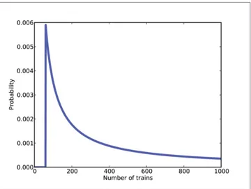
There are too many hypotheses to print, so I plotted the results in Figure 3-1. Not surprisingly, all values of N below 60 have been eliminated.
The most likely value, if you had to guess, is 60. That might not seem like a very good guess; after all, what are the chances that you just happened to see the train with the highest number? Nevertheless, if you want to maximize the chance of getting the answer exactly right, you should guess 60.
But maybe that’s not the right goal. An alternative is to compute the mean of the posterior distribution:
Figure 3-1. Posterior distribution for the locomotive problem, based on a uniform prior.
print Mean(suite)
Or you could use the very similar method provided by Pmf:
print suite.Mean()
The mean of the posterior is 333, so that might be a good guess if you wanted to minimize error. If you played this guessing game over and over, using the mean of the posterior as your estimate would minimize the mean squared error over the long run (see http:// en.wikipedia.org/wiki/Minimum_mean_square_error).
You can download this example from http://thinkbayes.com/train.py. For more infor‐ mation see “Working with the code” on page xi.
What about that prior?
To make any progress on the locomotive problem we had to make assumptions, and some of them were pretty arbitrary. In particular, we chose a uniform prior from 1 to
1000, without much justification for choosing 1000, or for choosing a uniform distri‐ bution.
It is not crazy to believe that a railroad company might operate 1000 locomotives, but a reasonable person might guess more or fewer. So we might wonder whether the pos‐ terior distribution is sensitive to these assumptions. With so little data—only one ob‐ servation—it probably is.
Recall that with a uniform prior from 1 to 1000, the mean of the posterior is 333. With an upper bound of 500, we get a posterior mean of 207, and with an upper bound of 2000, the posterior mean is 552.
So that’s bad. There are two ways to proceed: • Get more data.
• Get more background information.
With more data, posterior distributions based on different priors tend to converge. For example, suppose that in addition to train 60 we also see trains 30 and 90. We can update the distribution like this:
for data in [60, 30, 90]: suite.Update(data)
With these data, the means of the posteriors are
Upper Posterior Bound Mean 500 152 1000 164 2000 171
So the differences are smaller.
An alternative prior
If more data are not available, another option is to improve the priors by gathering more background information. It is probably not reasonable to assume that a train-operating company with 1000 locomotives is just as likely as a company with only 1.
With some effort, we could probably find a list of companies that operate locomotives in the area of observation. Or we could interview an expert in rail shipping to gather information about the typical size of companies.
But even without getting into the specifics of railroad economics, we can make some educated guesses. In most fields, there are many small companies, fewer medium-sized
companies, and only one or two very large companies. In fact, the distribution of com‐ pany sizes tends to follow a power law, as Robert Axtell reports in Science (see http:// www.sciencemag.org/content/293/5536/1818.full.pdf).
This law suggests that if there are 1000 companies with fewer than 10 locomotives, there might be 100 companies with 100 locomotives, 10 companies with 1000, and possibly one company with 10,000 locomotives.
Mathematically, a power law means that the number of companies with a given size is inversely proportional to size, or
We can construct a power law prior like this:
class Train(Dice):
def __init__(self, hypos, alpha=1.0): Pmf.__init__(self)
for hypo in hypos:
self.Set(hypo, hypo**(-alpha)) self.Normalize()
And here’s the code that constructs the prior:
hypos = range(1, 1001) suite = Train(hypos)
Again, the upper bound is arbitrary, but with a power law prior, the posterior is less sensitive to this choice.
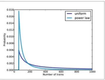
Figure 3-2 shows the new posterior based on the power law, compared to the posterior based on the uniform prior. Using the background information represented in the power law prior, we can all but eliminate values of N greater than 700.
Figure 3-2. Posterior distribution based on a power law prior, compared to a uniform prior.
Now the differences are much smaller. In fact, with an arbitrarily large upper bound, the mean converges on 134.
So the power law prior is more realistic, because it is based on general information about the size of companies, and it behaves better in practice.
You can download the examples in this section from http://thinkbayes.com/train3.py. For more information see “Working with the code” on page xi.
Credible intervals
Once you have computed a posterior distribution, it is often useful to summarize the results with a single point estimate or an interval. For point estimates it is common to use the mean, median, or the value with maximum likelihood.
For intervals we usually report two values computed so that there is a 90% chance that the unknown value falls between them (or any other probability). These values define a credible interval.
A simple way to compute a credible interval is to add up the probabilities in the posterior distribution and record the values that correspond to probabilities 5% and 95%. In other words, the 5th and 95th percentiles.
thinkbayes provides a function that computes percentiles:
def Percentile(pmf, percentage):
And here’s the code that uses it:
interval = Percentile(suite, 5), Percentile(suite, 95) print interval
For the previous example—the locomotive problem with a power law prior and three trains—the 90% credible interval is 91,243 . The width of this range suggests, correctly, that we are still quite uncertain about how many locomotives there are.
Cumulative distribution functions
In the previous section we computed percentiles by iterating through the values and probabilities in a Pmf. If we need to compute more than a few percentiles, it is more efficient to use a cumulative distribution function, or Cdf.
Cdfs and Pmfs are equivalent in the sense that they contain the same information about the distribution, and you can always convert from one to the other. The advantage of the Cdf is that you can compute percentiles more efficiently.
thinkbayes provides a Cdf class that represents a cumulative distribution function. Pmf
provides a method that makes the corresponding Cdf:
cdf = suite.MakeCdf()
And Cdf provides a function named Percentile
interval = cdf.Percentile(5), cdf.Percentile(95)
Converting from a Pmf to a Cdf takes time proportional to the number of values,
len(pmf). The Cdf stores the values and probabilities in sorted lists, so looking up a probability to get the corresponding value takes “log time”: that is, time proportional to the logarithm of the number of values. Looking up a value to get the corresponding probability is also logarithmic, so Cdfs are efficient for many calculations.
The examples in this section are in http://thinkbayes.com/train3.py. For more informa‐ tion see “Working with the code” on page xi.
1. Ruggles and Brodie, “An Empirical Approach to Economic Intelligence in World War II,” Journal of the American Statistical Association, Vol. 42, No. 237 (March 1947).
The German tank problem
During World War II, the Economic Warfare Division of the American Embassy in London used statistical analysis to estimate German production of tanks and other equipment.1
The Western Allies had captured log books, inventories, and repair records that included chassis and engine serial numbers for individual tanks.
Analysis of these records indicated that serial numbers were allocated by manufacturer and tank type in blocks of 100 numbers, that numbers in each block were used sequen‐ tially, and that not all numbers in each block were used. So the problem of estimating German tank production could be reduced, within each block of 100 numbers, to a form of the locomotive problem.
Based on this insight, American and British analysts produced estimates substantially lower than estimates from other forms of intelligence. And after the war, records indi‐ cated that they were substantially more accurate.
They performed similar analyses for tires, trucks, rockets, and other equipment, yielding accurate and actionable economic intelligence.
The German tank problem is historically interesting; it is also a nice example of real-world application of statistical estimation. So far many of the examples in this book have been toy problems, but it will not be long before we start solving real problems. I think it is an advantage of Bayesian analysis, especially with the computational approach we are taking, that it provides such a short path from a basic introduction to the research frontier.
Discussion
Among Bayesians, there are two approaches to choosing prior distributions. Some rec‐ ommend choosing the prior that best represents background information about the problem; in that case the prior is said to be informative. The problem with using an informative prior is that people might use different background information (or inter‐ pret it differently). So informative priors often seem subjective.
The alternative is a so-called uninformative prior, which is intended to be as unre‐ stricted as possible, in order to let the data speak for themselves. In some cases you can identify a unique prior that has some desirable property, like representing minimal prior information about the estimated quantity.
Uninformative priors are appealing because they seem more objective. But I am gen‐ erally in favor of using informative priors. Why? First, Bayesian analysis is always based on modeling decisions. Choosing the prior is one of those decisions, but it is not the only one, and it might not even be the most subjective. So even if an uninformative prior is more objective, the entire analysis is still subjective.
Also, for most practical problems, you are likely to be in one of two regimes: either you have a lot of data or not very much. If you have a lot of data, the choice of the prior doesn’t matter very much; informative and uninformative priors yield almost the same results. We’ll see an example like this in the next chapter.
But if, as in the locomotive problem, you don’t have much data, using relevant back‐ ground information (like the power law distribution) makes a big difference.
And if, as in the German tank problem, you have to make life-and-death decisions based on your results, you should probably use all of the information at your disposal, rather than maintaining the illusion of objectivity by pretending to know less than you do.
Exercises
Exercise 3-1.
To write a likelihood function for the locomotive problem, we had to answer this ques‐ tion: “If the railroad has N locomotives, what is the probability that we see number 60?” The answer depends on what sampling process we use when we observe the locomotive. In this chapter, I resolved the ambiguity by specifying that there is only one train-operating company (or only one that we care about).
But suppose instead that there are many companies with different numbers of trains. And suppose that you are equally likely to see any train operated by any company. In that case, the likelihood function is different because you are more likely to see a train operated by a large company.
As an exercise, implement the likelihood function for this variation of the locomotive problem, and compare the results.
CHAPTER 4
More Estimation
The Euro problem
In Information Theory, Inference, and Learning Algorithms, David MacKay poses this problem:
A statistical statement appeared in “The Guardian” on Friday January 4, 2002: When spun on edge 250 times, a Belgian one-euro coin came up heads 140 times and tails 110. ‘It looks very suspicious to me,’ said Barry Blight, a statistics lecturer at the London School of Economics. ‘If the coin were unbiased, the chance of getting a result as extreme as that would be less than 7%.’
But do these data give evidence that the coin is biased rather than fair?
To answer that question, we’ll proceed in two steps. The first is to estimate the probability that the coin lands face up. The second is to evaluate whether the data support the hypothesis that the coin is biased.
You can download the code in this section from http://thinkbayes.com/euro.py. For more information see “Working with the code” on page xi.
Any given coin has some probability, x, of landing heads up when spun on edge. It seems reasonable to believe that the value of x depends on some physical characteristics of the coin, primarily the distribution of weight.
If a coin is perfectly balanced, we expect x to be close to 50%, but for a lopsided coin, x
might be substantially different. We can use Bayes’s theorem and the observed data to estimate x.
Let’s define 101 hypotheses, where Hx is the hypothesis that the probability of heads is x%, for values from 0 to 100. I’ll start with a uniform prior where the probability of Hx
is the same for all x. We’ll come back later to consider other priors.
The likelihood function is relatively easy: If Hx is true, the probability of heads is x/ 100
and the probability of tails is 1 −x/ 100.
class Euro(Suite):
def Likelihood(self, data, hypo): x = hypo
if data == 'H': return x/100.0 else:
return 1 - x/100.0
Here’s the code that makes the suite and updates it:
suite = Euro(xrange(0, 101)) dataset = 'H' * 140 + 'T' * 110
for data in dataset: suite.Update(data)
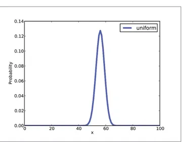
The result is in Figure 4-1.
Figure 4-1. Posterior distribution for the Euro problem on a uniform prior.
Summarizing the posterior
Again, there are several ways to summarize the posterior distribution. One option is to find the most likely value in the posterior distribution. thinkbayes provides a function that does that:
def MaximumLikelihood(pmf):
"""Returns the value with the highest probability.""" prob, val = max((prob, val) for val, prob in pmf.Items()) return val
In this case the result is 56, which is also the observed percentage of heads,
140 / 250 = 0.56%. So that suggests (correctly) that the observed percentage is the max‐ imum likelihood estimator for the population.
We might also summarize the posterior by computing the mean and median:
print 'Mean', suite.Mean()
print 'Median', thinkbayes.Percentile(suite, 50)
The mean is 55.95; the median is 56. Finally, we can compute a credible interval:
print 'CI', thinkbayes.CredibleInterval(suite, 90)
The result is 51,61 .
Now, getting back to the original question, we would like to know whether the coin is fair. We observe that the posterior credible interval does not include 50%, which suggests that the coin is not fair.
But that is not exactly the question we started with. MacKay asked, “ Do these data give evidence that the coin is biased rather than fair?” To answer that question, we will have to be more precise about what it means to say that data constitute evidence for a hy‐ pothesis. And that is the subject of the next chapter.
But before we go on, I want to address one possible source of confusion. Since we want to know whether the coin is fair, it might be tempting to ask for the probability that x
is 50%:
print suite.Prob(50)
The result is 0.021, but that value is almost meaningless. The decision to evaluate 101 hypotheses was arbitrary; we could have divided the range into more or fewer pieces, and if we had, the probability for any given hypothesis would be greater or less.
Swamping the priors
We started with a uniform prior, but that might not be a good choice. I can believe that if a coin is lopsided, x might deviate substantially from 50%, but it seems unlikely that the Belgian Euro coin is so imbalanced that x is 10% or 90%.
It might be more reasonable to choose a prior that gives higher probability to values of
x near 50% and lower probability to extreme values.
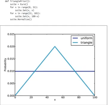
As an example, I constructed a triangular prior, shown in Figure 4-2. Here’s the code that constructs the prior:
def TrianglePrior(): suite = Euro()
for x in range(0, 51): suite.Set(x, x) for x in range(51, 101): suite.Set(x, 100-x) suite.Normalize()
Figure 4-2. Uniform and triangular priors for the Euro problem.
Figure 4-2 shows the result (and the uniform prior for comparison). Updating this prior with the same dataset yields the posterior distribution shown in Figure 4-3. Even with substantially different priors, the posterior distributions are very similar. The medians and the credible intervals are identical; the means differ by less than 0.5%.
This is an example of swamping the priors: with enough data, people who start with different priors will tend to converge on the same posterior.
Figure 4-3. Posterior distributions for the Euro problem.
Optimization
The code I have shown so far is meant to be easy to read, but it is not very efficient. In general, I like to develop code that is demonstrably correct, then check whether it is fast enough for my purposes. If so, there is no need to optimize. For this example, if we care about run time, there are several ways we can speed it up.
The first opportunity is to reduce the number of times we normalize the suite. In the original code, we call Update once for each spin.
dataset = 'H' * heads + 'T' * tails
for data in dataset: suite.Update(data)
And here’s what Update looks like:
def Update(self, data): for hypo in self.Values():
like = self.Likelihood(data, hypo) self.Mult(hypo, like)
return self.Normalize()
Each update iterates through the hypotheses, then calls Normalize, which iterates through the hypotheses again. We can save some time by doing all of the updates before normalizing.
Suite provides a method called UpdateSet that does exactly that. Here it is:
def UpdateSet(self, dataset): for data in dataset:
for hypo in self.Values():
like = self.Likelihood(data, hypo) self.Mult(hypo, like)
return self.Normalize()
And here’s how we can invoke it:
dataset = 'H' * heads + 'T' * tails suite.UpdateSet(dataset)
This optimization speeds things up, but the run time is still proportional to the amount of data. We can speed things up even more by rewriting Likelihood to process the entire dataset, rather than one spin at a time.
In the original version, data is a string that encodes either heads or tails:
def Likelihood(self, data, hypo): x = hypo / 100.0
if data == 'H': return x else:
return 1-x
As an alternative, we could encode the dataset as a tuple of two integers: the number of heads and tails. In that case Likelihood looks like this:
def Likelihood(self, data, hypo): x = hypo / 100.0
heads, tails = data
like = x**heads * (1-x)**tails return like
And then we can call Update like this:
heads, tails = 140, 110 suite.Update((heads, tails))
Since we have replaced repeated multiplication with exponentiation, this version takes the same time for any number of spins.
The beta distribution
There is one more optimization that solves this problem even faster.