Combinatorial Optimization
volume 1
Concepts of
Combinatorial Optimization
Edited by
First published 2010 in Great Britain and the United States by ISTE Ltd and John Wiley & Sons, Inc. Adapted and updated from Optimisation combinatoire volumes 1 to 5published 2005-2007 in France by Hermes Science/Lavoisier© LAVOISIER 2005, 2006, 2007
Apart from any fair dealing for the purposes of research or private study, or criticism or review, as permitted under the Copyright, Designs and Patents Act 1988, this publication may only be reproduced, stored or transmitted, in any form or by any means, with the prior permission in writing of the publishers, or in the case of reprographic reproduction in accordance with the terms and licenses issued by the CLA. Enquiries concerning reproduction outside these terms should be sent to the publishers at the undermentioned address:
ISTE Ltd John Wiley & Sons, Inc.
27-37 St George’s Road 111 River Street
London SW19 4EU Hoboken, NJ 07030
UK USA
www.iste.co.uk www.wiley.com
© ISTE Ltd 2010
The rights of Vangelis Th. Paschos to be identified as the author of this work have been asserted by him in accordance with the Copyright, Designs and Patents Act 1988.
Library of Congress Cataloging-in-Publication Data
Combinatorial optimization / edited by Vangelis Th. Paschos. v. cm.
Includes bibliographical references and index. Contents: v. 1. Concepts of combinatorial optimization
ISBN 978-1-84821-146-9 (set of 3 vols.) -- ISBN 978-1-84821-147-6 (v. 1) 1. Combinatorial optimization. 2. Programming (Mathematics)
I. Paschos, Vangelis Th. QA402.5.C545123 2010 519.6'4--dc22
2010018423
British Library Cataloguing-in-Publication Data
A CIP record for this book is available from the British Library ISBN 978-1-84821-146-9 (Set of 3 volumes)
ISBN 978-1-84821-147-6 (Volume 1)
Table of Contents
Preface . . . xiii
Vangelis Th. PASCHOS PART I.COMPLEXITY OF COMBINATORIAL OPTIMIZATION PROBLEMS . . . 1
Chapter 1. Basic Concepts in Algorithms and Complexity Theory . . . 3
Vangelis Th. PASCHOS 1.1. Algorithmic complexity . . . 3
1.2. Problem complexity . . . 4
1.3. The classes P, NP and NPO . . . 7
1.4. Karp and Turing reductions . . . 9
1.5. NP-completeness . . . 10
1.6. Two examples of NP-complete problems . . . 13
1.6.1. MIN VERTEX COVER . . . 14
1.6.2. MAX STABLE . . . 15
1.7. A few words on strong and weak NP-completeness . . . 16
1.8. A few other well-known complexity classes . . . 17
1.9. Bibliography . . . 18
Chapter 2. Randomized Complexity . . . 21
Jérémy BARBAY 2.1. Deterministic and probabilistic algorithms . . . 22
2.1.1. Complexity of a Las Vegas algorithm . . . 24
2.1.2. Probabilistic complexity of a problem . . . 26
2.2. Lower bound technique . . . 28
2.2.1. Definitions and notations . . . 28
2.2.2. Minimax theorem . . . 30
vi Combinatorial Optimization 1
2.3. Elementary intersection problem . . . 35
2.3.1. Upper bound . . . 35
2.3.2. Lower bound. . . 36
2.3.3. Probabilistic complexity . . . 37
2.4. Conclusion . . . 37
2.5 Bibliography . . . 37
PART II.CLASSICAL SOLUTION METHODS . . . 39
Chapter 3. Branch-and-Bound Methods . . . 41
Irène CHARON and Olivier HUDRY 3.1. Introduction . . . 41
3.2. Branch-and-bound method principles . . . 43
3.2.1. Principle of separation . . . 44
3.2.2. Pruning principles . . . 45
3.2.3. Developing the tree . . . 51
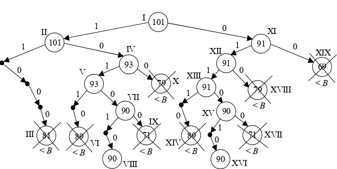
3.3. A detailed example: the binary knapsack problem . . . 54
3.3.1. Calculating the initial bound . . . 55
3.3.2. First principle of separation . . . 57
3.3.3. Pruning without evaluation . . . 58
3.3.4. Evaluation . . . 60
3.3.5. Complete execution of the branch-and-bound method for finding only one optimal solution . . . 61
3.3.6. First variant: finding all the optimal solutions . . . 63
3.3.7. Second variant: best first search strategy . . . 64
3.3.8. Third variant: second principle of separation . . . 65
3.4. Conclusion . . . 67
3.5. Bibliography . . . 68
Chapter 4. Dynamic Programming . . . 71
Bruno ESCOFFIER and Olivier SPANJAARD 4.1. Introduction . . . 71
4.2. A first example: crossing the bridge . . . 72
4.3. Formalization . . . 75
4.3.1. State space, decision set, transition function . . . 75
4.3.2. Feasible policies, comparison relationships and objectives . . . 77
4.4. Some other examples . . . 79
4.4.1. Stock management . . . 79
4.4.2. Shortest path bottleneck in a graph . . . 81
4.4.3. Knapsack problem . . . 82
4.5. Solution . . . 83
Table of Contents vii
4.5.2. Backward procedure . . . 85
4.5.3. Principles of optimality and monotonicity . . . 86
4.6. Solution of the examples . . . 88
4.6.1. Stock management . . . 88
4.6.2. Shortest path bottleneck . . . 89
4.6.3. Knapsack . . . 89
4.7. A few extensions . . . 90
4.7.1. Partial order and multicriteria optimization . . . 91
4.7.2. Dynamic programming with variables . . . 94
4.7.3. Generalized dynamic programming . . . 95
4.8. Conclusion . . . 98
4.9. Bibliography . . . 98
PART III.ELEMENTS FROM MATHEMATICAL PROGRAMMING . . . 101
Chapter 5. Mixed Integer Linear Programming Models for Combinatorial Optimization Problems . . . 103
Frédérico DELLA CROCE 5.1. Introduction . . . 103
5.1.1. Preliminaries . . . 103
5.1.2. The knapsack problem . . . 105
5.1.3. The bin-packing problem . . . 105
5.1.4. The set covering/set partitioning problem . . . 106
5.1.5. The minimum cost flow problem . . . 107
5.1.6. The maximum flow problem . . . 108
5.1.7. The transportation problem . . . 109
5.1.8. The assignment problem . . . 110
5.1.9. The shortest path problem . . . 111
5.2. General modeling techniques . . . 111
5.2.1. Min-max, max-min, min-abs models . . . 112
5.2.2. Handling logic conditions . . . 113
5.3. More advanced MILP models . . . 117
5.3.1. Location models . . . 117
5.3.2. Graphs and network models . . . 120
5.3.3. Machine scheduling models . . . 127
5.4. Conclusions . . . 132
5.5. Bibliography . . . 133
Chapter 6. Simplex Algorithms for Linear Programming . . . 135
Frédérico DELLA CROCE and Andrea GROSSO 6.1. Introduction . . . 135
viii Combinatorial Optimization 1
6.2.1. Optimality conditions and strong duality . . . 136
6.2.2. Symmetry of the duality relation . . . 137
6.2.3. Weak duality. . . 138
6.2.4. Economic interpretation of duality . . . 139
6.3. The primal simplex method . . . 140
6.3.1. Basic solutions . . . 140
6.3.2. Canonical form and reduced costs . . . 142
6.4. Bland’s rule . . . 145
6.4.1. Searching for a feasible solution . . . 146
6.5. Simplex methods for the dual problem . . . 147
6.5.1. The dual simplex method . . . 147
6.5.2. The primal–dual simplex algorithm . . . 149
6.6. Using reduced costs and pseudo-costs for integer programming . . . . 152
6.6.1. Using reduced costs for tightening variable bounds . . . 152
6.6.2. Pseudo-costs for integer programming . . . 153
6.7. Bibliography . . . 155
Chapter 7. A Survey of some Linear Programming Methods . . . 157
Pierre TOLLA 7.1. Introduction . . . 157
7.2. Dantzig’s simplex method . . . 158
7.2.1. Standard linear programming and the main results . . . 158
7.2.2. Principle of the simplex method . . . 159
7.2.3. Putting the problem into canonical form . . . 159
7.2.4. Stopping criterion, heuristics and pivoting . . . 160
7.3. Duality . . . 162
7.4. Khachiyan’s algorithm . . . 162
7.5. Interior methods . . . 165
7.5.1. Karmarkar’s projective algorithm . . . 165
7.5.2. Primal–dual methods and corrective predictive methods . . . 169
7.5.3. Mehrotra predictor–corrector method . . . 181
7.6. Conclusion . . . 186
7.7. Bibliography . . . 187
Chapter 8. Quadratic Optimization in 0–1 Variables . . . 189
Alain BILLIONNET 8.1. Introduction . . . 189
8.2. Pseudo-Boolean functions and set functions . . . 190
8.3. Formalization using pseudo-Boolean functions . . . 191
8.4. Quadratic pseudo-Boolean functions (qpBf) . . . 192
8.5. Integer optimum and continuous optimum of qpBfs . . . 194
Table of Contents ix
8.7. Posiforms and quadratic posiforms . . . 196
8.7.1. Posiform maximization and stability in a graph . . . 196
8.7.2. Implication graph associated with a quadratic posiform . . . 197
8.8. Optimizing a qpBf: special cases and polynomial cases . . . 198
8.8.1. Maximizing negative–positive functions . . . 198
8.8.2. Maximizing functions associated with k-trees . . . 199
8.8.3. Maximizing a quadratic posiform whose terms are associated with two consecutive arcs of a directed multigraph . . . 199
8.8.4. Quadratic pseudo-Boolean functions equal to the product of two linear functions . . . 199
8.9. Reductions, relaxations, linearizations, bound calculation and persistence . . . 200
8.9.1. Complementation . . . 200
8.9.2. Linearization . . . 201
8.9.3. Lagrangian duality . . . 202
8.9.4. Another linearization . . . 203
8.9.5. Convex quadratic relaxation . . . 203
8.9.6. Positive semi-definite relaxation . . . 204
8.9.7. Persistence . . . 206
8.10. Local optimum . . . 206
8.11. Exact algorithms and heuristic methods for optimizing qpBfs . . . 208
8.11.1. Different approaches . . . 208
8.11.2. An algorithm based on Lagrangian decomposition . . . 209
8.11.3. An algorithm based on convex quadratic programming . . . 210
8.12. Approximation algorithms . . . 211
8.12.1. A 2-approximation algorithm for maximizing a quadratic posiform . . . 211
8.12.2. MAX-SAT approximation . . . 213
8.13. Optimizing a quadratic pseudo-Boolean function with linear constraints . . . 213
8.13.1. Examples of formulations . . . 214
8.13.2. Some polynomial and pseudo-polynomial cases . . . 217
8.13.3. Complementation . . . 217
8.14. Linearization, convexification and Lagrangian relaxation for optimizing a qpBf with linear constraints . . . 220
8.14.1. Linearization . . . 221
8.14.2. Convexification . . . 222
8.14.3. Lagrangian duality . . . 223
8.15. ε-Approximation algorithms for optimizing a qpBf with linear constraints . . . 223
x Combinatorial Optimization 1
Chapter 9. Column Generation in Integer Linear Programming . . . 235
Irène LOISEAU, Alberto CESELLI, Nelson MACULAN and Matteo SALANI 9.1. Introduction . . . 235
9.2. A column generation method for a bounded variable linear programming problem . . . 236
9.3. An inequality to eliminate the generation of a 0–1 column . . . 238
9.4. Formulations for an integer linear program . . . 240
9.5. Solving an integer linear program using column generation . . . 243
9.5.1. Auxiliary problem (pricing problem) . . . 243
9.5.2. Branching . . . 244
9.6. Applications . . . 247
9.6.1. The p-medians problem . . . 247
9.6.2. Vehicle routing . . . 252
9.7. Bibliography . . . 255
Chapter 10. Polyhedral Approaches . . . 261
Ali Ridha MAHJOUB 10.1. Introduction . . . 261
10.2. Polyhedra, faces and facets . . . 265
10.2.1. Polyhedra, polytopes and dimension . . . 265
10.2.2. Faces and facets . . . 268
10.3. Combinatorial optimization and linear programming . . . 276
10.3.1. Associated polytope . . . 276
10.3.2. Extreme points and extreme rays . . . 279
10.4. Proof techniques . . . 282
10.4.1. Facet proof techniques . . . 283
10.4.2. Integrality techniques . . . 287
10.5. Integer polyhedra and min–max relations . . . 293
10.5.1. Duality and combinatorial optimization . . . 293
10.5.2. Totally unimodular matrices . . . 294
10.5.3. Totally dual integral systems . . . 296
10.5.4. Blocking and antiblocking polyhedral . . . 297
10.6. Cutting-plane method . . . 301
10.6.1. The Chvátal–Gomory method . . . 302
10.6.2. Cutting-plane algorithm . . . 304
10.6.3. Branch-and-cut algorithms. . . 305
10.6.4. Separation and optimization . . . 306
10.7. The maximum cut problem . . . 308
10.7.1. Spin glass models and the maximum cut problem . . . 309
10.7.2. The cut polytope . . . 310
10.8. The survivable network design problem . . . 313
Table of Contents xi
10.8.2. Valid inequalities and separation . . . 315
10.8.3. A branch-and-cut algorithm . . . 318
10.9. Conclusion . . . 319
10.10. Bibliography . . . 320
Chapter 11. Constraint Programming . . . 325
Claude LE PAPE 11.1. Introduction . . . 325
11.2. Problem definition . . . 327
11.3. Decision operators . . . 328
11.4. Propagation . . . 330
11.5. Heuristics . . . 333
11.5.1. Branching . . . 333
11.5.2. Exploration strategies . . . 335
11.6. Conclusion . . . 336
11.7. Bibliography . . . 336
List of Authors . . . 339
Index . . . 343
Preface
What is combinatorial optimization? There are, in my opinion, as many definitions as there are researchers in this domain, each one as valid as the other. For me, it is above all the art of understanding a real, natural problem, and being able to transform it into a mathematical model. It is the art of studying this model in order to extract its structural properties and the characteristics of the solutions of the modeled problem. It is the art of exploiting these characteristics in order to determine algorithms that calculate the solutions but also to show the limits in economy and efficiency of these algorithms. Lastly, it is the art of enriching or abstracting existing models in order to increase their strength, portability, and ability to describe mathematically (and computationally) other problems, which may or may not be similar to the problems that inspired the initial models.
Seen in this light, we can easily understand why combinatorial optimization is at the heart of the junction of scientific disciplines as rich and different as theoretical computer science, pure and applied, discrete and continuous mathematics, mathematical economics, and quantitative management. It is inspired by these, and enriches them all.
This book, Concepts of Combinatorial Optimization, is the first volume in a set entitled Combinatorial Optimization. It tries, along with the other volumes in the set, to embody the idea of combinatorial optimization. The subjects of this volume cover themes that are considered to constitute the hard core of combinatorial optimization. The book is divided into three parts:
– Part I: Complexity of Combinatorial Optimization Problems; – Part II: Classical Solution Methods;
xiv Combinatorial Optimization 1
In the first part, Chapter 1 introduces the fundamentals of the theory of (deterministic) complexity and of algorithm analysis. In Chapter 2, the context changes and we consider algorithms that make decisions by “tossing a coin”. At each stage of the resolution of a problem, several alternatives have to be considered, each one occurring with a certain probability. This is the context of probabilistic (or randomized) algorithms, which is described in this chapter.
In the second part some methods are introduced that make up the great classics of combinatorial optimization: branch-and-bound and dynamic programming. The former is perhaps the most well known and the most popular when we try to find an optimal solution to a difficult combinatorial optimization problem. Chapter 3 gives a thorough overview of this method as well as of some of the most well-known tree search methods based upon branch-and-bound. What can we say about dynamic programming, presented in Chapter 4? It has considerable reach and scope, and very many optimization problems have optimal solution algorithms that use it as their central method.
The third part is centered around mathematical programming, considered to be the heart of combinatorial optimization and operational research. In Chapter 5, a large number of linear models and an equally large number of combinatorial optimization problems are set out and discussed. In Chapter 6, the main simplex algorithms for linear programming, such as the primal simplex algorithm, the dual simplex algorithm, and the primal–dual simplex algorithm are introduced. Chapter 7 introduces some classical linear programming methods, while Chapter 8 introduces quadratic integer optimization methods. Chapter 9 describes a series of resolution methods currently widely in use, namely column generation. Chapter 10 focuses on polyhedral methods, almost 60 years old but still relevant to combinatorial optimization research. Lastly, Chapter 11 introduces a more contemporary, but extremely interesting, subject, namely constraint programming.
This book is intended for novice researchers, or even Master’s students, as much as for senior researchers. Master’s students will probably need a little basic knowledge of graph theory and mathematical (especially linear) programming to be able to read the book comfortably, even though the authors have been careful to give definitions of all the concepts they use in their chapters. In any case, to improve their knowledge of graph theory, readers are invited to consult a great, flagship book from one of our gurus, Claude Berge: Graphs and Hypergraphs, North Holland, 1973. For linear programming, there is a multitude of good books that the reader could consult, for example V. Chvátal, Linear Programming, W.H. Freeman, 1983, or M. Minoux, Programmation mathématique: théorie et algorithmes, Dunod, 1983.
Preface xv
lot of any university academic), have agreed to participate in the book by writing chapters in their areas of expertise and, at the same time, to take part in a very tricky exercise: writing chapters that are both educational and high-level science at the same time.
This work could never have come into being without the original proposal of Jean-Charles Pomerol, Vice President of the scientific committee at Hermes, and Sami Ménascé and Raphaël Ménascé, the heads of publications at ISTE. I give my warmest thanks to them for their insistence and encouragement. It is a pleasure to work with them as well as with Rupert Heywood, who has ingeniously translated the material in this book from the original French.
PART I
Chapter 1
Basic Concepts in Algorithms
and Complexity Theory
1.1. Algorithmic complexity
In algorithmic theory, a problem is a general question to which we wish to find an answer. This question usually has parameters or variables the values of which have yet to be determined. A problem is posed by giving a list of these parameters as well as the properties to which the answer must conform. An instance of a problem is obtained by giving explicit values to each of the parameters of the instanced problem. An algorithm is a sequence of elementary operations (variable affectation, tests, forks, etc.) that, when given an instance of a problem as input, gives the solution of this problem as output after execution of the final operation.
The two most important parameters for measuring the quality of an algorithm are: itsexecution timeand thememory spacethat it uses. The first parameter is expressed
in terms of the number of instructions necessary to run the algorithm. The use of the number of instructions as a unit of time is justified by the fact that the same program will use the same number of instructions on two different machines but the time taken will vary, depending on the respective speeds of the machines. We generally consider that an instruction equates to an elementary operation, for example an assignment, a test, an addition, a multiplication, a trace, etc. What we call thecomplexity in timeor
simply thecomplexityof an algorithm gives us an indication of the time it will take to
solve a problem of a given size. In reality this is a function that associates an order of
Chapter written by Vangelis Th. PASCHOS.
4 Combinatorial Optimization 1
magnitude1of the number of instructions necessary for the solution of a given problem with the size of an instance of that problem. The second parameter corresponds to the number of memory units used by the algorithm to solve a problem. Thecomplexity in spaceis a function that associates an order of magnitude of the number of memory
units used for the operations necessary for the solution of a given problem with the size of an instance of that problem.
There are several sets of hypotheses concerning the “standard configuration” that we use as a basis for measuring the complexity of an algorithm. The most commonly used framework is the one known as “worst-case”. Here, the complexity of an algo-rithm is the number of operations carried out on the instance that represents the worst configuration, amongst those of a fixed size, for its execution; this is the framework used in most of this book. However, it is not the only framework for analyzing the complexity of an algorithm. Another framework often used is “average analysis”. This kind of analysis consists of finding, for a fixed size (of the instance)n, the aver-age execution time of an algorithm on all the instances of sizen; we assume that for this analysis the probability of each instance occurring follows a specific distribution pattern. More often than not, this distribution pattern is considered to be uniform. There are three main reasons for the worst-case analysis being used more often than the average analysis. The first is psychological: the worst-case result tells us for cer-tain that the algorithm being analyzed can never have a level of complexity higher than that shown by this analysis; in other words, the result we have obtained gives us an upper bound on the complexity of our algorithm. The second reason is mathe-matical: results from a worst-case analysis are often easier to obtain than those from an average analysis, which very often requires mathematical tools and more complex analysis. The third reason is “analysis portability”: the validity of an average analysis is limited by the assumptions made about the distribution pattern of the instances; if the assumptions change, then the original analysis is no longer valid.
1.2. Problem complexity
The definition of the complexity of an algorithm can be easily transposed to prob-lems. Informally,the complexity of a problem is equal to the complexity of the best algorithm that solves it(this definition is valid independently of which framework we
use).
Let us take a sizenand a functionf(n). Thus:
–TIMEf(n)is the class of problems for which the complexity (in time) of an instance of sizenis inO(f(n)).
1. Orders of magnitude are defined as follows: given two functionsfandg:f =O(g)if and only if∃(k, k′
)∈(R+,R)such thatfkg+k′
;f=o(g)if and only iflimn→∞(f /g) = 0;
Basic Concepts in Algorithms and Complexity Theory 5
–SPACEf(n)is the class of problems that can be solved, for an instance of sizen, by using a memory space ofO(f(n)).
We can now specify the following general classes of complexity:
–Pis the class of all the problems that can be solved in a time that is a polynomial function of their instance size, that isP=∪∞
k= 0 TIMEnk.
–EXPTIMEis the class of problems that can be solved in a time that is an expo-nential function of their instance size, that isEXPTIME=∪∞
k= 0 TIME2n k
.
–PSPACE is the class of all the problems that can be solved using a mem-ory space that is a polynomial function of their instance size, that is PSPACE = ∪∞
k= 0 SPACEnk.
With respect to the classes that we have just defined, we have the following re-lations: P ⊆ PSPACE ⊆ EXPTIMEandP ⊂ EXPTIME. Knowing whether the inclusions of the first relation are strict or not is still an open problem.
Almost all combinatorial optimization problems can be classified, from an algo-rithmic complexity point of view, into two large categories. Polynomial problems
can be solved optimally by algorithms of polynomial complexity, that is inO(nk), wherekis a constant independent ofn(this is the classPthat we have already de-fined).Non-polynomialproblems are those for which the best algorithms (those giving
an optimum solution) are of a “super-polynomial” complexity, that is inO(f(n)g(n) ), wheref andgare increasing functions innandlimn→∞g(n) =∞. All these prob-lems contain the classEXPTIME.
The definition of any algorithmic problem (and even more so in the case of any combinatorial optimization problem) comprises two parts. The first gives the instance of the problem, that is the type of its variables (a graph, a set, a logical expression, etc.). The second part gives the type and properties to which the expected solution must conform. In the complexity theory case, algorithmic problems can be classified into three categories:
–decision problems;
–optimum value calculation problems;
–optimization problems.
Decision problems are questions concerning the existence, for a given instance, of
a configuration such that this configuration itself, or its value, conforms to certain properties. The solution to a decision problem is an answer to the question associated with the problem. In other words, this solution can be:
– either “yes, such a configuration does exist”;
6 Combinatorial Optimization 1
Let us consider as an example the conjunctive normal form satisfiability problem, known in the literature asSAT: “Given a setUofnBoolean variablesx1 , . . . , xnand a setCofmclauses2C1 , . . . , Cm, is there a model for the expressionφ=C1 ∧. . .∧Cm; i.e. is there an assignment of the values 0 or 1 to the variables such that φ = 1?”. For an instanceφof this problem, ifφallows a model then the solution (the correct answer) isyes, otherwise the solution isno.
Let us now consider theMIN TSPproblem, defined as follows: given a complete graphKn overnvertices for which each edgee∈E(Kn)has a valued(e)>0, we are looking for a Hamiltonian cycleH ⊂E(a partial closely related graph such that each vertex is of 2 degrees) that minimizes the quantity
e∈Hd(e). Let us assume that for this problem we have, as well as the complete graph Kn and the vectord, costs on the edgesKn of a constantKand that we are looking not to determine the smallest (in terms of total cost) Hamiltonian cycle, but rather to answer the following question: “Does there exist a Hamiltonian cycle of total distance less than or equal toK?”. Here, once more, the solution is eitheryesif such a cycle exists, ornoif it
does not.
Foroptimum value calculation problems, we are looking to calculatethe value of the optimum solution(and not the solution itself).
In the case of theMIN TSPfor example, the optimum associated value calculation problem comes down to calculating the cost of the smallest Hamiltonian cycle, and not the cycle itself.
Optimization problems, which are naturally of interest to us in this book, are those
for which we are looking to establish the best solution amongst those satisfying certain properties given by the very definition of the problem. An optimization problem may be seen as a mathematical program of the form:
opt v(x)
x∈CI
wherexis the vector describing the solution3,v(x)is theobjective function,CI is the problem’s constraint set, set out for the instanceI(in other words,CI sets out both the instance and the properties of the solution that we are looking to find for this instance), andopt∈ {max,min}. Anoptimum solutionofI is a vectorx∗ ∈ argopt{v(x) :
x∈CI}. The quantityv(x∗)is known as theobjective valueorvalueof the problem. A solutionx∈CI is known as afeasible solution.
2. We associate twoliteralsxand¯xwith a Boolean variablex, that is the variable itself and its negation; a clause is a disjunction of the literals.
Basic Concepts in Algorithms and Complexity Theory 7
Let us consider the problemMIN WEIGHTED VERTEX COVER4. An instance of this problem (given by the information from the incident matrixA, of dimensionm×n, of a graphG(V, E)of ordernwith|E| =mand a vectorw, of dimensionnof the costs of the edges ofV), can be expressed in terms of a linear program in integers as
follows: ⎧
⎨
⎩
min w·x A.x1
x∈ {0,1}n
wherexis a vector from 0, 1 of dimensionnsuch thatxi = 1if the vertexvi ∈ V is included in the solution,xi = 0if it is not included. The block ofmconstraints
A.x1expresses the fact that for each edge at least one of these extremes must be included in the solution. The feasible solutions are all the transversals ofGand the optimum solution is a transversal ofGof minimum total weight, that is a transversal corresponding to a feasible vector consisting of a maximum number of 1.
The solution to an optimization problem includes an evaluation of the optimum value. Therefore, an optimum value calculation problem can be associated with an optimization problem. Moreover, optimization problems always have a decisional variant as shown in theMIN TSPexample above.
1.3. The classes P, NP and NPO
Let us consider a decision problemΠ. If for any instanceIofΠa solution (that is a correct answer to the question that statesΠ) ofIcan be found algorithmically in polynomial time, that is inO(|I|k)stages, where|I|is the size ofI, thenΠis called apolynomial problemand the algorithm that solves it apolynomial algorithm(let us
remember that polynomial problems make up thePclass).
For reasons of simplicity, we will assume in what follows that the solution to a decision problem is:
– either “yes, such a solution exists, and this is it”;
– or “no, such a solution does not exist”.
In other words, if, to solve a problem, we could consult an “oracle”, it would provide us with an answer of not just ayesornobut also, in the first case, a certificate
4. Given a graphG(V, E)of ordern, in theMIN VERTEX COVERproblem we are looking to find a smallest transversal ofG, that is a setV′
⊆ V such that for every edge(u, v) ∈ E, eitheru∈V′, or
v∈V′of minimum size; we denote by
8 Combinatorial Optimization 1
proving the veracity of theyes. This testimony is simply a solution proposal that the
oracle “asserts” as being the real solution to our problem.
Let us consider the decision problems for which the validity of the certificate can be verified in polynomial time. These problems form the classNP.
DEFINITION1.1.– A decision problemΠis inNPif the validity of all solutions ofΠ is verifiable in polynomial time.
For example, theSATproblem belongs toNP. Indeed, given the assignment of the values 0, 1 to the variables of an instanceφof this problem, we can, with at mostnm
applications of the connector∨, decide whether the proposed assignment is a model forφ, that is whether it satisfies all the clauses.
Therefore, we can easily see that the decisional variant ofMIN TSPseen previously also belongs toNP.
Definition 1.1 can be extended to optimization problems. Let us consider an opti-mization problemΠand let us assume that each instanceIofΠconforms to the three following properties:
1) The feasibility of a solution can be verified in polynomial time. 2) The value of a feasible solution can be calculated in polynomial time.
3) There is at least one feasible solution that can be calculated in polynomial time.
Thus,Πbelongs to the classNPO. In other words,the classNPOis the class of optimization problems for which the decisional variant is inNP. We can therefore define the classPOof optimization problems for which the decisional variant belongs to the classP. In other words,POis the class of problems that can be optimally solved in polynomial time.
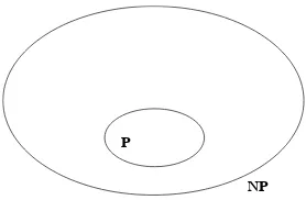
We note that the classNPhas been defined (see definition 1.1) without explicit reference to the optimum solution of its problems, but by reference to the verification of a given solution. Evidently, the condition of belonging toP being stronger than that of belonging toNP(what can be solved can be verified), we have the obvious inclusion of :P⊆NP(Figure 1.1).
“What is the complexity of the problems inNP\P?”. The best general result on the complexity of the solution of problems fromNPis as follows [GAR 79].
THEOREM1.1.– For any problemΠ∈NP, there is a polynomialpΠ such that each
instanceIofΠcan be solved by an algorithm of complexityO(2pΠ(|I|)).
Basic Concepts in Algorithms and Complexity Theory 9
NP P
Figure 1.1.PandNP(under the assumptionP=NP)
and although almost all researchers in complexity are completely convinced of its veracity, it has still not been proved. The question “IsP equal to or different from NP?”is the biggest open question in computer science and one of the best known in
mathematics.
1.4. Karp and Turing reductions
As we have seen, problems inNP\Pare considered to be algorithmically more difficult than problems inP. A large number of problems inNP\Pare very strongly bound to each other through the concept ofpolynomial reduction.
The principle of reducing a problemΠto a problemΠ′consists of considering the problemΠas a specific case of Π′,moduloa slight transformation. If this transfor-mation is polynomial, and we know that we can solveΠ′in polynomial time, we will also be able to solveΠin polynomial time. Reduction is thus a means of transferring the result of solving one problem to another; in the same way it is a tool for classifying problems according to the level of difficulty of their solution.
We will start with the classic Karp reduction (for the classNP) [GAR 79, KAR 72]. This links two decision problems by the possibility of their optimum (and simultane-ous) solution in polynomial time. In the following, given a problemΠ, letIΠ be all of its instances (we assume that each instanceI ∈ IΠ is identifiable in polynomial time in|I|). LetOΠ be the subset ofIΠ for which the solution isyes;OΠ is also known as the set ofyes-instances (or positive instances) ofΠ.
DEFINITION 1.2.– Given two decision problemsΠ1 andΠ2 , a Karp reduction (or
10 Combinatorial Optimization 1
A Karp reduction of a decision problemΠ1 to a decision problemΠ2 implies the existence of an algorithm A1 forΠ1 that uses an algorithmA2for Π2 . Given any instanceI1 ∈ IΠ 1, the algorithmA1constructs an instanceI2 ∈ IΠ 2; it executes the algorithmA2, which calculates a solution onI2 , thenA1transforms this solution into a solution forΠ1 onI1 . IfA2is polynomial, thenA1is also polynomial.
Following on from this, we can state another reduction, known in the literature as theTuring reduction, which is better adapted to optimization problems. In what
follows, we define a problem Π as a couple(IΠ ,SolΠ ), whereSolΠ is the set of solutions forΠ(we denote bySolΠ (I)the set of solutions for the instanceI∈ IΠ ). DEFINITION1.3.– A Turing reduction of a problemΠ1 to a problemΠ2 is an
algo-rithmA1that solvesΠ1 by using (possibly several times) an algorithmA2forΠ2 in
such a way that ifA2is polynomial, thenA1is also polynomial.
The Karp and Turing reductions are transitive: ifΠ1 is reduced (by one of these two reductions) to Π2 andΠ2 is reduced toΠ3 , thenΠ1 reduces to Π3 . We can therefore see that both reductions preserve membership of the classPin the sense that ifΠreduces toΠ′andΠ′∈P, thenΠ∈P.
For more details on both the Karp and Turing reductions refer to [AUS 99, GAR 79, PAS 04]. In Garey and Johnson [GAR 79] (Chapter 5) there is also a very interesting historical summary of the development of the ideas and terms that have led to the structure of complexity theory as we know it today.
1.5. NP-completeness
From the definition of the two reductions in the preceding section, ifΠ′ reduces toΠ, thenΠ can reasonably be considered as at least as difficult as Π′ (regarding their solution by polynomial algorithms), in the sense that a polynomial algorithm forΠwould have sufficed to solve not onlyΠitself, but equallyΠ′. Let us confine ourselves to the Karp reduction. By using it, we can highlight a problemΠ∗ ∈ NP such that any other problemΠ ∈ NPreduces toΠ∗ [COO 71, GAR 79, FAG 74]. Such a problem is, as we have mentioned, the most difficult problem of the classNP. Therefore we can show [GAR 79, KAR 72] that there are other problemsΠ∗′ ∈ NP such thatΠ∗reduces toΠ∗′. In this way we expose a family of problems such that any problem inNPreduces (remembering that the Karp reduction is transitive) to one of its problems. This family has, of course, the following properties:
– It is made up of the most difficult problems ofNP.
Basic Concepts in Algorithms and Complexity Theory 11
The problems from this family areNP-completeproblems and the class of these
problems is called theNP-completeclass.
DEFINITION1.4.– A decision problemΠisNP-complete if, and only if, it fulfills the following two conditions:
1)Π∈NP;
2)∀Π′∈NP,Π′reduces toΠby a Karp reduction.
Of course, a notion ofNP-completeness very similar to that of definition 1.4 can also be based on the Turing reduction.
The following application of definition 1.3 is very often used to show the NP-completeness of a problem. LetΠ1 = (IΠ 1,SolΠ 1)andΠ2 = (IΠ 2,SolΠ 2)be two problems, and let(f, g)be a pair of functions, which can be calculated in polynomial time, where:
–f :IΠ 1→ IΠ2 is such that for any instanceI∈ IΠ 1,f(I)∈ IΠ 2;
–g : IΠ 1 ×SolΠ 2 → SolΠ1 is such that for every pair (I, S) ∈ (IΠ 1 × SolΠ 2(f(I))),g(I, S)∈SolΠ 1(I).
Let us assume that there is a polynomial algorithmAfor the problemΠ2 . In this case, the algorithmf◦A◦gis a (polynomial) Turing reduction.
A problem that fulfills condition 2 of definition 1.4 (without necessarily checking condition 1) is calledNP-hard5. It follows thata decision problemΠisNP-complete
if and only if it belongs toNPand it isNP-hard.
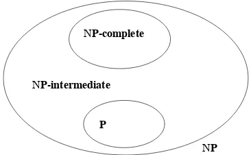
With the classNP-complete, we can further refine (Figure 1.2) the world ofNP. Of course, ifP=NP, the three classes from Figure 1.2 coincide; moreover, under the assumptionP=NP, the classesPandNP-complete do not intersect.
Let us denote byNP-intermediate the classNP\(P∪NP−complete). Informally, this concerns the class of problems of intermediate difficulty, that is problems that are more difficult than those fromPbut easier than those fromNP-complete. More for-mally, for two complexity classesCandC′such thatC′ ⊆C, and a reductionR pre-serving the membership ofC′, a problem isC-intermediate if it is neitherC-complete underR, nor belongs toC′. Under the Karp reduction, the classNP-intermediate is not empty [LAD 75].
Let us note that the idea ofNP-completeness goes hand in hand with decision problems. When dealing with optimization problems, the appropriate term, used in
12 Combinatorial Optimization 1
NP P
NP-complete
NP-intermediate
Figure 1.2.P,NPandNP-complete(under the assumptionP=NP)
the literature, isNP-hard6.A problem ofNPOisNP-hard if and only if its decisional variant is anNP-completeproblem.
The problemSATwas the first problem shown to be NP-complete (the proof of this important result can be found in [COO 71]). The reduction used (often called
generic reduction) is based on the theory of recursive languages and Turing
ma-chines (see [HOP 79, LEW 81] for more details and depth on the Turing machine concept; also, language-problem correspondence is very well described in [GAR 79, LEW 81]). The general idea of generic reduction, also often called the “Cook–Levin technique (or theory)”, is as follows: For a generic decision (language) problem belonging to NP, we describe, using a normal conjunctive form, the working of a non-deterministic algorithm (Turing machine) that solves (decides) this problem (lan-guage).
The second problem shown to beNP-complete [GAR 79, KAR 72] was the variant ofSAT, written 3SAT, where no clause contains more than three literals. The reduction here is fromSAT[GAR 79, PAP 81]. More generally, for allk3, thekSATproblems (that is the problems defined on normal conjunctive forms where each clause contains no more thankliterals) are allNP-complete.
It must be noted that the problem 2SAT, where all normal conjunctive form clauses contain at most two literals, is polynomial [EVE 76]. It should also be noted that in [KAR 72], where there is a list of the first 21NP-complete problems, the problem of linear programming in real numbers was mentioned as a probable problem from the
6. There is a clash with this term when it is used for optimization problems and when it is used in the sense of property 2 of definition 1.4, where it means that a decision problemΠis harder than any other decision problemΠ′
Basic Concepts in Algorithms and Complexity Theory 13
classNP-intermediate. It was shown, seven years later ([KHA 79] and also [ASP 80], an English translation of [KHA 79]), that this problem is inP.
The reference onNP-completeness is the volume by Garey and Johnson [GAR 79]. In the appendix,A list ofNP-complete problems, there is a long list ofNP-complete
problems with several commentaries for each one and for their limited versions. For many years, this list has been regularly updated by Johnson in theJournal of Algo-rithmsreview. This update, supplemented by numerous commentaries, appears under
the title:The NP-completeness column: an ongoing guide.
“What is the relationship between optimization and decision for NP-complete problems?”. The following theory [AUS 95, CRE 93, PAZ 81] attempts to give an answer.
THEOREM1.2.– LetΠbe a problem ofNPOand let us assume that the decisional version ofΠ, writtenΠd, isNP-complete. It follows that a polynomial Turing
reduc-tion exists betweenΠdandΠ.
In other words, the decision versions (such as those we have considered in this chapter) and optimization versions of anNP-complete problem are of equivalent al-gorithmic difficulty. However, the question of the existence of a problemNPOfor which the optimization version is more difficult to solve than its decisional counter-part remains open.
1.6. Two examples of NP-complete problems
Given a problemΠ, the most conventional way to show itsNP-completeness con-sists of making a Turing or Karp reduction of anNP-completeΠ′problem toΠ. In practical terms, the proof ofNP-completeness forΠis divided into three stages:
1) proof of membership ofΠtoNP; 2) choice ofΠ′;
3) building the functionsf andg(see definition 1.3) and showing that they can both be calculated in polynomial time.
In the following, we show that MIN VERTEX COVER(G(V, E), K) and MAX STABLE(G(V, E), K), the decisional variants ofMIN VERTEX COVERand of MAX STABLE7, respectively, areNP-complete. These two problems are defined as fol-lows. MIN VERTEX COVER(G(V, E), K): given a graphGand a constantK |V|, does there exist in Ga transversalV′ ⊆ V less than or equal in size toK? MAX
7. Given a graphG(V, E)of magnituden, we are trying to find a stable set of maximum size, that is a setV′
⊆V such that∀(u, v)∈V′ ×V′,
14 Combinatorial Optimization 1
STABLE SET(G(V, E), K): given a graphGand a constantK|V|, does there exist inGa stable setV′⊆V of greater than or equal in size toK?
1.6.1. MIN VERTEX COVER
The proof of membership ofMIN VERTEX COVER(G(V, E), K) toNPis very simple and so has been omitted here. We will therefore show the completeness of this problem forNP. We will transform an instance φ(U,C)from 3SAT, withU = {x1 , . . . , xn}andC={C1 , . . . , Cm}, into an instance(G(V, E), K)ofMIN VERTEX COVER.
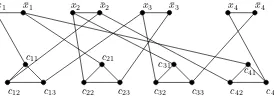
This graph is made up of two component sets, joined by edges. The first compo-nent is made up of2nverticesx1 ,x¯1 , . . . , xn,x¯nandnedges(xi,x¯i),i= 1, . . . , n, which join the vertices in pairs. The second is made up ofmvertex-disjoint triangles (that is ofmcliques with three vertices). For a clauseCi, we denote the three vertices of the corresponding triangle byci1 ,ci2 andci3 . In fact, the first set of components, for which each vertex corresponds to a literal, serves to define the truth values of the solution for 3SAT; the second set of components corresponds to the clauses, and each vertex is associated with a literal of its clause. These triangles are used to verify the satisfaction of the clauses. To finish, we add3m“unifying” edges that link each vertex of each “triangle-clause” to its corresponding “literal-vertex”. Let us note that exactly three unifying edges go from (the vertices of) each triangle, one per vertex of the trian-gle. Finally, we stateK=n+ 2m. It is easy to see that the transformation ofφ(U,C) toG(V, E)happens in polynomial time inmax{m, n}since|V| = 2n+ 3mand |E|=n+ 6m.
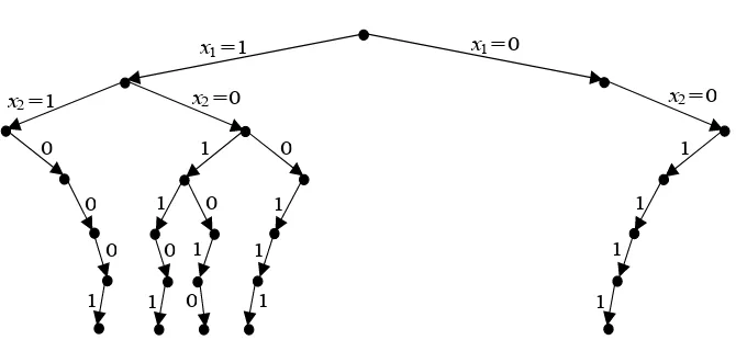
As an example of the transformation described above, let us consider the instance
φ= (x1 ∨x¯2 ∨x3 )∧(¯x1 ∨x2 ∨x¯3 )∧(x2 ∨x3 ∨x¯4 )∧(¯x1 ∨x¯2 ∨x4 )from 3SAT. The graphG(V, E)forMIN VERTEX COVERis given in Figure 1.3. In this case,K= 12.
x1 ¯x1 x2 ¯x2 x3 x¯3 x4 x¯4
c1 1 c1 2 c1 3
c2 1 c2 2 c2 3
c3 1 c3 2 c3 3
c4 1 c4 2 c4 3 Figure 1.3.The graph associated with the expression
(x1∨x¯2∨x3)∧(¯x1∨x2∨x¯3)∧(x2∨x3∨x¯4)∧(¯x1∨x¯2∨x4)
Basic Concepts in Algorithms and Complexity Theory 15
Let us first show that the condition is necessary. Let us assume that there is a polynomial algorithmAthat answers the question “Is there inGa transversalV′ ⊆V of size|V′|K?”, and, if so, returnsV′. Let us execute it withK=n+ 2m. If the answer fromAisyes, then the transversal must be of a sizeequalton+2m. In fact, any transversal needs at leastnvertices in order to cover thenedges corresponding to the variables ofφ(one vertex per edge) and2mvertices to cover the edges ofmtriangles (two vertices per triangle). As a result, if Aanswers yes, it will have calculated a
transversal of exactlyn+ 2mvertices.
In the light of the previous observation, given such a transversalV′, we state that
xi = 1if the extremityxi of the edge(xi,x¯i)is taken inV′; if the extremityx¯i is included, then we state thatx¯i = 1, that isxi = 0. We claim that this assignment of the truth values to the variables satisfies φ. Indeed, since only one extremity of each edge(xi,x¯i)is taken inV′,only one literal is set to 1 for each variableand, in consequence, the assignment in question is coherent (one, and only one, truth value is assigned to each literal). Moreover, let us consider a triangleTiofGcorresponding to the clauseCi; let us denote its vertices byci1 ,ci2 andci3 , and let us assume that the last two belong toV′. Let us also assume that the unifying edge having as an extremity the vertexci1 is the edge(ci1 , ℓk),ℓk being one of the literals associated with the variablexk. Sinceci1 ∈/ V′,ℓk belongs to it, that isℓk = 1, and the existence of the edge(ci1 , ℓk)means that the literalℓkbelongs to the clauseCi. This is proved by setting ℓk to 1. By iterating this argument for each clause, the need for the condition is proved. Furthermore, let us note that obtaining the assignment of the truth values to the variables ofφis done in polynomial time.
Let us now show that the condition is also good enough. Given an assignment of truth values satisfying the expressionφ, let us construct inGa transversalV′ of sizen+ 2m. To start with, for each variablexi, ifxi = 1, then the extremityxiof the edge(xi,x¯i)is put inV′; otherwise, the extremityx¯i of the edge(xi,x¯i)is put there. We thereby cover the edges of type(xi,x¯i),i = 1, . . . , n, and one unifying edge per triangle. LetTi(corresponding to the clauseCi),i= 1, . . . , m, be a triangle and let(ℓk, ci1 )be the unifying edge covered by the setting to 1 ofℓk. We therefore put the verticesci2 andci3 inV′; these vertices cover both the edges ofTi and the two unifying edges having as extremitiesci2 andci3 , respectively. By iterating this operation for each triangle, a transversalV′of sizen+ 2mis eventually constructed in polynomial time.
1.6.2. MAX STABLE
16 Combinatorial Optimization 1
Let us consider a graphG(V, E)of magnitudenhavingmedges and let us denote byAits incidence matrix8. Let us also consider the expression ofMIN VERTEX COVER as a linear program in whole numbers and the transformations that follow:
⎧ ⎨
⎩
min 1·y A·y1
y∈ {0,1}n
⇔ ⎧ ⎨
⎩
min 1·y
2.1−A·y1
y∈ {0,1}n
⇔ ⎧ ⎨
⎩
min 1·y A·
1−y 1
y∈ {0,1}n
y= 1 −x ⇐⇒
⎧ ⎨
⎩
min 1· 1−x
A·x1
x∈ {0,1}n
⇔ ⎧ ⎨
⎩
max 1·x A·x1
x∈ {0,1}n
We note that the last program in the series is nothing more than the linear program (in whole numbers) ofMAX STABLE. Furthermore, this series of equivalents indicates that if a solution vectorxforMAX STABLEis given, then the vectory = 1−x(that is the vectory where we interchange the “1” and the “0” regardingx) is a feasible solution forMIN VERTEX COVER. Furthermore, ifxcontains at leastK “1” (that is the size of the stable set is at least equal toK), then the solution vector deduced for MIN VERTEX COVERcontains at mostn−K“1” (that is the size of the transversal is at most equal ton−K). Since the functionx→1−xis polynomial, then so is the described transformation.
1.7. A few words on strong and weak NP-completeness
LetΠbe a problem andIan instance ofΠof size|I|. We denote bymax(I)the highest number that appears inI. Let us note thatmax(I)can be exponential inn. An algorithm forΠis known aspseudo-polynomialif it is polynomial in|I|andmax(I) (ifmax(I)is exponential in|I|, then this algorithm is exponential forI).
DEFINITION 1.5.– An optimization problem is NP-complete in the strong sense (strongly NP-complete) if the problem isNP-complete because of its structure and not because of the size of the numbers that appear in its instances. A problem isNP -complete in the weak sense (weaklyNP-complete) if it isNP-complete because of its valuations (that is max(I)affects the complexity of the algorithms that solve it).
Let us consider on the one hand theSATproblems, orMIN VERTEX COVER prob-lems, or even the MAX STABLEproblems seen previously, and on the other hand the KNAPSACKproblem for which the decisional variant is defined as: “given a maxi-mum costb,nobjects{1, . . . , n}of respective valuesaiand respective costsci b,
Basic Concepts in Algorithms and Complexity Theory 17
i = 1, . . . , n, and a constant K, is there a subset of objects for which the sum of the values is at least equal to K without the sum of the costs of these objects ex-ceedingb?”. This problem is the most well-known weaklyNP-complete problem. Its intrinsic difficulty is not due to its structure, as is the case for the previous three prob-lems where no large number affects the description of their instances, but rather due to the values ofaiandcithat do affect the specification of the instance ofKNAPSACK. In Chapter 4 (see also Volume 2, Chapter 8), we find a dynamic programming algorithm that solves this problem in linear time for the highest value ofaiand in log-arithmic time for the highest value ofci. This means that if this value is a polynomial ofn, then the algorithm is also polynomial, and if the value is exponential inn, the algorithm itself is of exponential complexity.
The result below [GAR 79, PAS 04] follows the borders between strongly and weaklyNP-complete problems. If a problemΠis stronglyNP-complete, then it can-not be solved by a pseudo-polynomial algorithm, unlessP=NP.
1.8. A few other well-known complexity classes
In this section, we briefly present a few supplementary complexity classes that we will encounter in the following chapters (for more details, see [BAL 88, GAR 79, PAP 94]). Introductions to some complexity classes can also be found in [AUS 99, VAZ 01].
Let us consider a decision problemΠand a generic instanceIofΠdefined on a data structureS(a graph, for example) and a decision constantK. From the definition of the classNP, we can deduce that if there is a solution giving the answeryesforΠ onI, and if this solution is submitted for verification, then the answer for any correct verification algorithm will always beyes. On the other hand, if such a solution does
not exist, then any solution proposal submitted for verification will always bring about anoanswer from any correct verification algorithm.
Let us consider the following decisional variant ofMIN TSP, denoted by co-MIN TSP: “given Kn,dandK, is it true that there is no Hamiltonian cycle of a total distance less than or equal to K?”. How can we guarantee that the answer for an instance of this problem is yes? This questions leads on to that of this problem’s
membership of the class NP. We come across the same situation for a great many problems inNP\P(assuming thatP=NP).
We denote byIΠ the set of all the instances of a decision problemΠ ∈ NPand byOΠ the subset ofIΠ for which the solution isyes, that is the set ofyes-instances
18 Combinatorial Optimization 1
NP co-NP
P
Figure 1.4.P,NPandco-NP(under the conditionsP=NPandNP=co-NP)
up the class co-NP. In other words, co-NP = {Π : Π¯ ∈ NP}. It is surmised that NP = co-NP. This surmise is considered as being “stronger” thanP = NP, in the sense that it is possible thatP = NP, even if NP = co-NP(but ifP = NP, then NP=co-NP).
Obviously, for a decision problemΠ ∈P, the problemΠ¯ also belongs toP; as a result,P⊆NP∩co-NP.
A decision problemΠbelongs toRPif there is a polynomialpand an algorithmA such that, for any instance I: if I ∈ OΠ , then the algorithm gives a decision in polynomial time for at least half of the candidate solutions (certificates)S, such that |S| p(|I|), that are submitted to it for verification of their feasibility; if, on the other hand,I /∈ OΠ (that is ifI ∈ IΠ \ OΠ ), then for any proposed solutionSwith |S| p(|I|),ArejectsS in polynomial time. A problemΠ ∈co-RPif and only if
¯
Π∈RP, whereΠ¯is defined as before. We have the following relationship betweenP, RPandNP:P⊆RP⊆NP. For a very simple and intuitive proof of this relationship, see [VAZ 01].
The class ZPP(an abbreviation of zero-error probabilistic polynomial time) is
the class of decision problems that allow a randomized algorithm (for this subject see [MOT 95] and Chapter 2) that always ends up giving the correct answer to the question “I ∈ OΠ ?”, with, on average, a polynomial complexity. A problemΠ be-longs to ZPP if and only if Π belongs to RP∩co-RP. In other words, ZPP = RP∩co-RP.
1.9. Bibliography
Basic Concepts in Algorithms and Complexity Theory 19
[AUS 95] AUSIELLOG., CRESCENZIP., PROTASIM., “Approximate solutions of NP opti-mization problems”,Theoret. Comput. Sci., vol. 150, p. 1–55, 1995.
[AUS 99] AUSIELLOG., CRESCENZIP., GAMBOSIG., KANNV., MARCHETTI-SPACCAME-LAA., PROTASIM.,Complexity and Approximation. Combinatorial Optimization Prob-lems and their Approximability properties, Springer-Verlag, Berlin, 1999.
[BAL 88] BALCÀZAR J.L., DIAZ J., GABARRÒ J., Structural Complexity, vol. 1 and 2, Springer-Verlag, Berlin, 1988.
[COO 71] COOKS.A., “The complexity of theorem-proving procedures”, Proc. STOC’71, p. 151–158, 1971.
[CRE 93] CRESCENZIP., SILVESTRIR., “Average measure, descriptive complexity and ap-proximation of minimization problems”,Int. J. Foundations Comput. Sci., vol. 4, p. 15–30, 1993.
[EVE 76] EVENS., ITAIA., SHAMIRA., “On the complexity of timetable and multicommod-ity flow problems”,SIAM J. Comput., vol. 5, p. 691–703, 1976.
[FAG 74] FAGINR., “Generalized first-order spectra and polynomial-time recognizable sets”, KARPR.M., Ed.,Complexity of Computations, p. 43–73, American Mathematics Society, 1974.
[GAR 79] GAREYM.R., JOHNSOND.S.,Computers and Intractability. A Guide to the The-ory of NP-completeness, W. H. Freeman, San Francisco, 1979.
[HOP 79] HOPCROFTJ.E., ULLMANJ.D.,Introduction to Automata Theory, Languages and Computation, Addison-Wesley, 1979.
[KAR 72] KARP R.M., “Reducibility among combinatorial problems”, MILLER R.E., THATCHERJ.W., Eds.,Complexity of computer computations, p. 85–103, Plenum Press, New York, 1972.
[KHA 79] KHACHIAN L.G., “A polynomial algorithm for linear programming”, Dokladi Akademiy Nauk SSSR, vol. 244, p. 1093–1096, 1979.
[LAD 75] LADNERR.E., “On the structure of polynomial time reducibility”, J. Assoc. Com-put. Mach., vol. 22, p. 155–171, 1975.
[LEW 81] LEWIS H.R., PAPADIMITRIOU C.H., Elements of the Theory of Computation, Prentice-Hall, New Jersey, 1981.
[MOT 95] MOTWANIR., RAGHAVAN P., Randomized Algorithms, Cambridge University Press, Cambridge, 1995.
[PAP 81] PAPADIMITRIOUC.H., STEIGLITZK., Combinatorial Optimization: Algorithms and Complexity, Prentice-Hall, New Jersey, 1981.
[PAP 94] PAPADIMITRIOUC.H.,Computational Complexity, Addison-Wesley, 1994. [PAS 04] PASCHOSV.TH.,Complexité et approximation polynomiale, Hermes, Paris, 2004. [PAZ 81] PAZA., MORANS., “Non deterministic polynomial optimization problems and their
approximations”,Theoret. Comput. Sci., vol. 15, p. 251–277, 1981.
Chapter 2
Randomized Complexity
A deterministic algorithm is “a method of solution, by the application of a rule, a finite number of times” (Chapter 1). This definition extends to probabilistic algorithms by allowing probabilistic rules, or by giving a distribution of probability over a set of deterministic algorithms. By definition, probabilistic algorithms are potentially more
powerful than their deterministic counterparts: the class of probabilistic algorithms contains the class of deterministic algorithms. It is therefore natural to consider prob-abilistic algorithms for solving the hardest combinatorial optimization problems, all the more so because probabilistic algorithms are often simpler than their deterministic counterparts.
A deterministic algorithm is correct if it solves each instance in a valid way. In the context of probabilistic algorithms for which the execution depends both on the instance and on the randomization of the algorithm, we consider the correct complex-ity of algorithms for any instance and any randomization, but also the complexcomplex-ity of algorithms such that for each instanceI, the probability that the algorithm correctly solvesIis higher than a constant (typically1/2).
In the context of combinatorial optimization, we consider algorithms for which the resultapproximatesthe solution of the problem set. We then examine both the complexity of the algorithm and thequalityof the approximations that it gives. We can, without loss of generality, limit ourselves to the problems of minimizing a cost function, in which case we look to minimize both the complexity of the algorithm and the cost of the approximation that it produces. Depending on whether we examine the complexity or the cost of the approximation generated, the terms are different but the
22 Combinatorial Optimization 1
techniques are similar: in both cases, we are looking to minimize a measure of the performance of the algorithm. This performance, for a probabilistic algorithm and a given instanceI, is defined as the average of the performance of the corresponding deterministic algorithm onI.
The aim of this chapter is to show that the analysis techniques used to study the complexity of probabilistic algorithms can be just as easily used to analyze the ap-proximation quality of combinatorial optimization algorithms. In section 2.1, we give a more formal definition of the concepts and notations generally used in the study of the complexity of probabilistic algorithms, and we introduce a basic problem that is used to illustrate the most simple results of this chapter. In section 2.2, we give and prove the basic results that allow us to prove lower bounds for the performance of probabilistic algorithms for a given problem. These results can often be used as they stand, but it is important to understand their causes in order to adapt them to less appropriate situations. The most common technique for proving an upper bound to the performance of the best probabilistic algorithm for a given problem is to ana-lyze the performance of the probabilistic algorithm, and for this purpose there are as many techniques as there are algorithms: for this reason we do not describe a general method, but instead give an example of analysis in section 2.3.
2.1. Deterministic and probabilistic algorithms
Analgorithmis a method for solving a problem using a finite number of rule ap-plications. In the computer science context, an algorithm is a precise description of the stages to be run through in order to carry out a calculation or a specific task. A
deterministic algorithmis an algorithm such that the choice of each rule to be ap-plied is deterministic. Aprobabilistic algorithmcan be defined in a similar way by a probabilistic distribution over the deterministic algorithms, or by giving a proba-bilistic distribution over the rules of the algorithm. In both cases, the data received by the algorithm make up theinstanceof the problem to be solved, and the choice of algorithm or rules makes up therandomizationof the execution.
Randomized Complexity 23
(Monte Carlo)
RP∩coRP
(Las Vegas)
RP coRP
P
Figure 2.1.Complexity classes relative to probabilistic algorithms that run in polynomial time
Problems that can be solved using Monte Carlo algorithms running in polynomial time make up the complexity classRP. Among these, problems that can be resolved by deterministic algorithms running in polynomial time make up the complexity classP. In a similar way, the classco-RPis made up of the set of problems that can be solved in polynomial time by a probabilistic algorithm that always accepts a positive instance, but refuses a negative instance with a probability of at least1/2. If a problem is in ZPP=RP∩co-RP, it allows an algorithm of each kind, and so allows an algorithm that is a combination of both, which always accepts positive instances and refuses negative instances, but in an unlimited time. The execution time of algorithms of this type can be random, but they always find a correct result. These algorithms are called “Las Vegas”: their result is certain, but their execution time is random, a bit like a martingale with a sufficiently large initial stake.
Another useful complexity class concerns probabilistic algorithms that can make mistakes both by accepting and by refusing instances of the class BPP, formed by problems that can be solved in polynomial time by a probabilistic algorithm refusing a positive instance or accepting a negative instance with a probability of at most1/4. Just as forRP, the value of1/4is arbitrary and can be replaced by1/2−p(n)for any polynomialp(n)without losing the important properties ofRP(but the value of1/2 would not be suitable here, see [MOT 95, p. 22]).
24 Combinatorial Optimization 1
EXAMPLE.– A classic problem is thebin-packingproblem: given a list of objects of heightsL={x1 , . . . , xn}, between0and1, we must make vertical stacks of objects
in such a way that the height of each stack does not exceed 1, and such that there is a minimum number of stacks. This problem isNP-complete and the approximation of the optimal numberµof stacks is a classic combinatorial optimization problem. Even if it is not a decision problem, it can be categorized in the same classes. It is enough to consider the following variant: given a list of the weights of objects
L = {x1 , . . . , xn}, and a number of stacks M, can these n objects be organized
into M stacks, without any of them exceeding one unit of height? Any algorithm approximatingµby a valuemsuch thatPr[m =µ] 3/4(if need be by iterating the same algorithm several times) allows us to decide whetherM stacks will suffice (m M) without ever being wrong whenM is not sufficient (M < µ m), and with a probability of being wrong of at most1/4 ifM is sufficient (Pr[µ < m =
M]1/4): the decision problem is inRP!
2.1.1. Complexity of a Las Vegas algorithm
Given a cost function over the operations carried out by the algorithm, the com-plexity of an algorithmAon an instanceIis the sum of the costs of the instructions corresponding to the execution ofAonI. The algorithms solving this same problem are compared by their complexity. Thetime complexityC(A, I)of an algorithmAon an instanceI corresponds to the number of instructions carried out byAwhen it is executed to solveI.
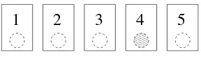
EXAMPLE.–
000 000 000 000 000
111 111 111 111 111
1
2
3
4
5
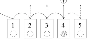
Figure 2.2.An instance of the hidden coin problem: one silver coin amongst four copper coins, the coins being hidden by cards
The hidden coin problem is another abstract problem that we will use to illustrate the different ideas of this chapter. We have a row ofncards. Each card hides a coin, which can be a copper coin or a silver coin. Thehidden coin problemis to decide whether the row contains at least one silver coin.
Randomized Complexity 25
– A deterministic algorithm uncovers coins in a fixed order.
– A potential algorithm chooses half of the coins randomly and uniformly, uncov-ers them, accepts the instance if there is a silver coin, and otherwise refuses. This algorithm always refuses an instance that does not contain a silver coin (therefore a negative instance), and accepts any instance containing at least one silver coin (there-fore positive) with a probability of at least1/2: therefore it is a Monte Carlo algorithm. – Another potential algorithm uncovers coins in a random order until it has found a silver coin, or it has uncovered all of the coins: this algorithm always gives the right answer, but the number of coins uncovered is a random variable that depends on the chosen order: it is therefore a Las Vegas algorithm.
In a configuration that has only one silver coin hidden under the second card from the right, the algorithm that uncovers coins from left to right will uncovern−1coins, the algorithm that uncovers coins from right to left will only uncover2coins.
000 000 000 000 000
111 111 111 111 111
1
2
3
4
5
+
Figure 2.3.The algorithm choosing coins from left to right: dotted lines show the possible executions, and solid lines show the executions on this instance. The answer of the algorithm
is positive because the row contains a silver coin
Let F = {I1 , . . . , I|F|} be a finite set of instances, and A an algorithm for these instances. The complexity C(A, F) of A on F can be defined in several ways. The set of values taken by the complexity of A on the instances