APPENDIX A: SPARKS
This section is meant for people who do most of their programming in FORTRAN. FORTRAN has the distinction of being essentially the earliest higher level programming language, developed about 1957 by a group at IBM. Since then it and its derivatives have become established as the primary
language for scientific and engineering computation. But, with our greater understanding of the process of creating programs has come a realization of the deficiencies of FORTRAN. Creating a program is properly thought of as taking a real world problem and translating it into a computer solution. Concepts in the real world such as a geneology tree or a queue of airplanes must be translated into computer concepts. A language is good if it enables one to describe these abstractions of the real world in a natural way. Perhaps because of its very early development, FORTRAN lacks many such features. In this appendix we explore the idea of writing a preprocessor for FORTRAN which inexpensively adds some of these missing features.
A preprocessor is a program which translates statements written in a language X
into FORTRAN. In our case X is called SPARKS. Such a program is normally called a compiler so why give it the special name preprocessor? A preprocessor is distinguished from a compiler in the following way: the source and target language have many statements in common.
Such a translator has many advantages. Most importantly it preserves a close connection with FORTRAN. Despite FORTRAN's many negative attributes, it has several practical pluses: 1) it is almost always available and compilers are often good, 2) there is a language standard which allows a degree of portability not obtainable with other languages, 3) there are extensive subroutine libraries, and 4) there is a large labor force familiar with it. These reasons give FORTRAN a strong hold in the industrial marketplace. A structured FORTRAN translator preserves these virtues while it augments the language with improved syntactical constructs and other useful features.
Another consideration is that at many installations a nicely structured language is unavailable. In this event a translator provides a simple means for
In order to see the difference between FORTRAN and SPARKS consider writing a program which searches for X in the sorted array of integers A (N), N 100. The output is the integer J which is either zero if X is not found or A(J) = X, 1
J N. The method used here is the well known binary search algorithm. The FORTRAN version looks something like this:
SUBROUTINE BINS (A,N,X,J) IMPLICIT INTEGER (A - Z) DIMENSION A(100)
BOT= 1 TOP= N J = 0
100 IF (BOT. GT. TOP) RETURN MID = (BOT + TOP)/2
IF (X. GE. A (MID)) GO TO 101 TOP = MID - 1
GO TO 100
101 IF (X. EQ. A (MID)) GO TO 102 BOT = MID + 1
GO TO 100 102 J = MID RETURN
END
This may not be the "best" way to write this program, but it is a reasonable attempt. Now we write this algorithm in SPARKS.
IMPLICIT INTEGER (A - Z)
The difference between these two algorithms may not be dramatic, but it is significant. The WHILE and CASE statements allow the algorithm to be described in a more natural way. The program can be read from top to bottom without your eyes constantly jumping up and down the page. When such
improvements are consistently adopted in a large software project, the resulting code is bound to be easier to comprehend.
The reserved words and special symbols are:
BY CASE CYCLE DO ELSE ENDCASE ENDIF EOJ EXIT FOR IF LOOP REPEAT UNTIL WHILE TO THEN : ; //
Reserved words must always be surrounded by blanks. Reserved means they cannot be used by the programmer as variables.
We now define the SPARKS statements by giving their FORTRAN equivalents. In the following any reference to the term "statements" is meant to include both SPARKS and FORTRAN statements. There are six basic SPARKS statements, two which improve the testing of cases and four which improve the description of looping.
IF cond THEN IF(.NOT. (cond)) GO TO 100 S1 S1
ELSE GO TO 101 S2 100 S2
ENDIF 101 CONTINUE
S1 and S2 are arbitrary size groups of statements. Cond must be a legal
FORTRAN conditional. The ELSE clause is optional but the ENDIF is required and it always terminates the innermost IF.
S1,S2, ...,Sn+1 are arbitrary size groups of statements. Cond1, cond2, ..., condn
are legal FORTRAN conditionals. The symbol ELSE surrounded by colons designates that Sn+l will be automatically executed if all previous conditions are false. This part of the case statement is optional.
WHILE cond DO 100 IF(.NOT. (cond)) GO TO 101 S S
REPEAT GO TO 100 101 CONTINUE
S is an arbitrary group of statements and cond a legal FORTRAN conditional. LOOP 100 CONTINUE
S S
UNTIL cond REPEAT IF(.NOT. (cond)) GO TO 100
S and cond are the same as for the while statement immediately preceding. LOOP 100 CONTINUE
S S
REPEAT GO TO 100 101 CONTINUE S is an arbitrary size group of statements. FOR vble = expl TO exp2 BY exp3 DO S
REPEAT
This has a translation of: vble = expl GO TO 100
102 vble = vble + exp3
GO TO 102 101 CONTINUE
The three expressions exp1, exp2, exp3 are allowed to be arbitrary FORTRAN arithmetic expressions of any type. Similarly vble may be of any type. However, the comparison test is made against integer zero. Since exp2 and exp3 are re-evaluated each time through the loop, care must be taken in its use.
EXIT is a SPARKS statement which causes a transfer of control to the first statement outside of the innermost LOOP-REPEAT statement which contains it. One example of its use is:
LOOP 100 CONTINUE S1 S1
IF cond THEN EXIT IF(.NOT. (cond)) GO TO 102 ENDIF GO TO 101
S2 102 CONTINUE REPEAT S2
GO TO 100 101 CONTINUE
A generalization of this statement allows EXIT to be used within any of the four SPARKS looping statements: WHILE, LOOP, LOOP-UNTIL and FOR. When executed, EXIT branches to the statement immediately following the innermost looping statement which contains it.
The statement CYCLE is also used within any SPARKS looping statement. Its execution causes a branch to the end of the innermost loop which contains it. A test may be made and if passed the next iteration is taken. An example of the use of EXIT and CYCLE follow.
CASE IF(.NOT. (cond1) GO TO 103 : cond1 : EXIT GO TO 102
: cond2 : CYCLE IF(.NOT. (cond2)) GO TO 104 ENDCASE 103 GO TO 101
S2 CONTINUE REPEAT 104 S2
GO TO 100 101 CONTINUE 102
EOJ or end of job must appear at the end of the entire SPARKS program. As a statement, it must appear somewhere in columns 7 through 72 and surrounded by blanks.
ENDIF is used to terminate the IF and ENDCASE to terminate the CASE
statement. REPEAT terminates the looping statements WHILE, LOOP and FOR. Labels follow the FORTRAN convention of being numeric and in columns one to five.
The use of doubleslash is as a delimiter for comments. Thus one can write //This is a comment//
and all characters within the double slashes will be ignored. Comments are restricted to one line and FORTRAN comments are allowed.
The semi-colon can be used to include more than one statement on a single line For example, beginning in column one the statement
99999 A = B + C; C = D + E; X = A
would be legal in SPARKS. To include a semicolon in a hollerith field it should be followed by a second semicolon. This will be deleted in the resulting
We are now ready to describe the operation of the translator. Two design approaches are feasible. The first is a table-driven method which scans a program and recognizes keywords. This approach is essentially the way a compiler works in that it requires a scanner, a symbol table (though limited), very limited parsing and the generation of object (FORTRAN) code. A second approach is to write a general macro preprocessor and then to define each SPARKS statement as a new macro. Such a processor is usually small and allows the user to easily define new constructs. However, these processors tend to be slower than the approach of direct translation. Moreover, it is hard to build in the appropriate error detection and recovery facilities which are sorely needed if SPARKS is to be used seriously. Therefore, we have chosen the first approach. Figure A.1 contains a flow description of the translator.
Figure A.1: Overview of SPARKS Translator
The main processing loop consists of determining the next statement and
branching within a large CASE. This does whatever translation into FORTRAN is necessary. When EOJ is found the loop is broken and the program is
concluded.
Extensions
Below is a list of possible extensions for SPARKS. Some are relatively easy to implement, while others require a great deal of effort.
E.1 Special cases of the CASE statement
CASE SGN : exp: CASE: integer variable: : .EQ.0 : S1 : 1 : S1
: .LT.0 : S2 and : 2 : S2 : .GT.0 : S3
ENDCASE : n : Sn ENDCASE
The first gets translated into the FORTRAN arithmetic IF statement. The second form is translated into a FORTRAN computed go to.
E.2 A simple form of the FOR statement would look like LOOP exp TIMES
S REPEAT
where exp is an expression which evaluates to a non-negative integer. The statements meaning can be described by the SPARKS for statement:
FOR ITEMP = 1 TO exp DO S
REPEAT
E.3 If F appears in column one then all subsequent cards are assumed to be pure FORTRAN. They are passed directly to the output until an F is encountered in column one.
E.4 Add the capability of profiling a program by determining the number of executions of each loop during a single execution and the value of conditional expressions.
HINT: For each subroutine declare a set of variables which can be inserted after encountering a WHILE, LOOP, REPEAT, FOR, THEN or ELSE statement. At the end of each subroutine a write statement prints the values of these counters. E.5 Add the multiple replacement statement so that
A = B = C = D + E is translated into
C = D + E; B = C; A = B
E.6 Add the vector replacement statement so that (A,B,C) = (X + Y, 10,2*E)
produces A = X + Y: B = 10 ; C = 2*E E.7 Add an array "fill" statement so that NAME(*) exp1,exp2,exp3
gets translated into
NAME(1) = exp1; NAME(2) = exp2; NAME(3) = exp3
E.8 Introduce appropriate syntax and reasonable conventions so that SPARKs programs can be recursive.
HINT: Mutually recursive programs are gathered together in a module,
E.9 Add a character string capability to SPARKS.
E.10 Add an internal procedure capability to aid the programmer in doing top-down program refinement.
E.11 Attach sequence numbers to the resulting FORTRAN output which relates each statement back to the original SPARKS statement which generated it. This is particularly helpful for debugging.
E.12 Along with the indented SPARKS source print a number which represents the level of nesting of each statement.
E.13 Generalize the EXIT statement so that upon its execution it can be assigned a value, e.g.,
LOOP S1
IF condl THEN EXIT : exp1: ENDIF S2
IF cond2 THEN EXIT : exp2: ENDIF S3
REPEAT
will assign either expl or exp2 as the value of the variable EXIT.
E.14 Supply a simplified read and write statement. For example, allow for hollerith strings to be included within quotes and translated to the nH x1 ... xn format.
All further questions about the definition of SPARKS should be addressed to: Chairman, SPARKS Users Group
Los Angeles, California 9007
To receive a complete ANSI FORTRAN version of SPARKS send $20.00 (for postage and handling) to Dr. Ellis Horowitz at the above address.
PREAMBLE
Recognition of professional status by the public depends not only on skill and dedication but also on adherence to a recognized code of Professional Conduct. The following Code sets forth the general principles (Canons), professional ideals (Ethical Considerations), and mandatory rules (Disciplinary Rules) applicable to each ACM Member.
The verbs "shall" (imperative) and "should" (encouragement) are used purposefully in the Code. The Canons and Ethical Considerations are not, however, binding rules. Each Disciplinary Rule is binding on each individual Member of ACM. Failure to observe the Disciplinary Rules subjects the Member to admonition, suspension, or expulsion from the Association as provided by the Constitution and Bylaws. The term "member(s)" is used in the Code. The
Disciplinary Rules of the Code apply, however, only to the classes of
CANON 1
An ACM member shall act at all times with integrity. Ethical Considerations
EC1.1. An ACM member shall properly qualify himself when expressing an opinion outside his areas of competence. A member is encouraged to express his opinion on subjects within his areas of competence.
EC1.2. An ACM member shall preface an partisan statements about information processing by indicating clearly on whose behalf they are made.
EC1.3. An ACM member shall act faithfully on behalf of his employers or clients.
Disciplinary Rules
DR1.1.1. An ACM member shall not intentionally misrepresent his
qualifications or credentials to present or prospective employers or clients. DR1.1.2. An ACM member shall not make deliberately false or deceptive statements as to the present or expected state of affairs in any aspect of the capability, delivery, or use of information processing systems.
DR1.2.1. An ACM member shall not intentionally conceal or misrepresent on whose behalf any partisan statements are made.
DR1.3.1. An ACM member acting or employed as a consultant shall, prior to accepting information from a prospective client, inform the client of all factors of which the member is aware which may affect the proper performance of the task.
DR1.3.2. An ACM member shall disclose any interest of which he is aware which does or may conflict with his duty to a present or prospective employer or client.
CANON 2
An ACM member should strive to increase his competence and the competence and prestige of the profession.
Ethical Considerations
EC2.1. An ACM member is encouraged to extend public knowledge,
understanding, and appreciation of information processing, and to oppose any false or deceptive statements relating to information processing of which he is aware.
EC2.2 An ACM member shall not use his professional credentials to misrepresent his competence.
EC2.3. An ACM member shall undertake only those professional assignments and commitments for which he is qualified.
EC2.4. An ACM member shall strive to design and develop systems that adequately perform the intended functions and that satisfy his employer's or client's operational needs.
EC2.5. An ACM member should maintain and increase his competence through a program of continuing education encompassing the techniques, technical standards, and practices in his fields of professional activity.
EC2.6. An ACM member should provide opportunity and encouragement for professional development and advancement of both professionals and those aspiring to become professionals.
Disciplinary Rules
DR2.2.1. An ACM member shall not use his professional credentials to misrepresent his competence.
DR2.3.1. An ACM member shall not undertake professional assignments without adequate preparation in the circumstances.
which he knows or should know he is not competent or cannot become
adequately competent without acquiring the assistance of a professional who is competent to perform the assignment.
CANON 3
An ACM member shall accept responsibility for his work. Ethical Considerations
EC3.1. An ACM member shall accept only those assignments for which there is reasonable expectancy of meeting requirements or specifications, and shall perform his assignments in a professional manner.
Disciplinary Rules
DR3.1.1. An ACM member shall not neglect any professional assignment which has been accepted.
DR3.1.2. An ACM member shall keep his employer or client properly informed on the progress of his assignments.
DR3.1.3. An ACM member shall not attempt to exonerate himself from, or to limit, his liability to his clients for his personal malpractice.
CANON 4
An ACM member shall act with professional responsibility. Ethical Considerations
EC4.1 An ACM member shall not use his membership in ACM improperly for professional advantage or to misrepresent the authority of his statements.
EC4.2. An ACM member shall conduct professional activities on a high plane. EC4.3. An ACM member is encouraged to uphold and improve the professional standards of the Association through participation in their formulation,
establishment, and enforcement. Disciplinary Rules
DR4.1.1. An ACM member shall not speak on behalf of the Association or any of its subgroups without proper authority.
DR4.1.2. An ACM member shall not knowingly misrepresent the policies and views of the Association or any of its subgroups.
DR4.1.3. An ACM member shall preface partisan statements about information processing by indicating clearly on whose behalf they are made.
DR4.2.1. An ACM member shall not maliciously injure the professional reputation of any other person.
DR4.2.2. An ACM member shall not use the services of or his membership in the Association to gain unfair advantage.
CANON 5
An ACM member should use his special knowledge and skills for the advancement of human welfare.
Ethical Considerations
EC5.1. An ACM member should consider the health, privacy, and general welfare of the public in the performance of his work.
EC5.2. An ACM member, whenever dealing with data concerning individuals, shall always consider the principle of the individual's privacy and seek the following:
--To minimize the data collected.
--To limit authorized access to the data. --To provide proper security for the data.
--To determine the required retention period of the data. --To ensure proper disposal of the data.
Disciplinary rules
DR5.2.1. An ACM member shall express his professional opinion to his employers or clients regarding any adverse consequences to the public which might result from work proposed to him.
APPENDIX C: ALGORITHM
INDEX BY CHAPTER
CHAPTER 1--INTRODUCTION
Exchange sorting--SORT 1.3 Binary search--BINSRCH 1.3 FIBONACCI 1.4
Filling a magic square--MAGIC 1.4 CHAPTER 2--ARRAYS
Polynomial addition--PADD 2.2 Fibonacci polynomials--MAIN 2.2
Sparse matrix transpose--TRANSPOSE 2.3
Sparse matrix transpose--FAST-TRANSPOSE 2.3 Sparse matrix multiplication--MMULT 2.3
CHAPTER 3--STACKS AND QUEUES Sequential stacks--ADD, DELETE 3.1 Sequential queues--ADDQ, DELETEQ 3.1
Circular sequential queues--ADDQ, DELETEQ 3.1 Path through a maze--PATH 3.2
Translating infix to postfix--POSTFIX 3.3 M-stacks sequential--ADD, DELETE 3.4 CHAPTER 4--LINKED LISTS
Create a list with 2 nodes--CREATE 2 4.1 Insert a node in a list--INSERT 4.1
Delete a node from a list--DELETE 4.1 Linked stacks--ADDS, DELETES 4.2 Linked queues--ADDQ, DELETEQ 4.2 Finding a new node--GETNODE 4.3 Initializing available space--INIT 4.3
Returning a node to available space--RET 4.3 Linked polynomial addition--PADD 4.4 Erasing a linked list--ERASE 4.4
Erasing a circular list--CERASE 4.4
Circular linked polynomial addition--CPADD 4.4 Inverting a linked list--INVERT 4.5
Concatenating two lists--CONCATENATE 4.5 Circular list insertion--INSERT-FRONT 4.5 Length of a circular list--LENGTH 4.5
Erasing a linked sparse matrix--MERASE 4.7 Doubly linked list--DDELETE, DINSERT 4.8 First fit allocation--FF, ALLOCATE 4.8
Returning freed blocks--FREE
General lists--COPY, EQUAL, DEPTH 4.9 Erasing a list with reference counts--ERASE 4.9
Garbage collection--DRIVER, MARK 1, MARK 2 4.10 Compacting storage--COMPACT 4.10
Strings--SINSERT 4.11
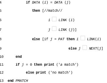
Finding a pattern--FIND, NFIND, PMATCH, FAIL 4.11 Initializing available space in FORTRAN-INIT 4.12 Initializing available space in PASCAL-INIT 4.12
FORTRAN node routines--COEP, SCOEF, EXP, SEXP, LINK, SLINK 4.12 CHAPTER 5--TREES
Inorder traversal--INORDER,INORDER1,2,3 5.4 Preorder traversal--PREORDER 5.4
Postorder traversal--POSTORDER 5.4 Copy a binary tree--COPY 5.5
Equivalence of binary trees--EQUAL 5.5
Traversing a threaded binary tree--TINORDER 5.6 Insertion in a threaded tree--INSERT-RIGHT 5.6 Disjoint set union--U, F, UNION, FIND 5.8 Decision trees--EIGHTCOINS 5.8
Game playing--VE,AB(alpha-beta) 5.8 CHAPTER 6--GRAPHS
Depth first search--DFS 6.2 Breadth first search--BFS 6.2
Connected components--COMP 6.2 Minimum spanning tree--KRUSKAL 6.2
Shortest path, single source--SHORTEST-PATH 6.3 Shortest paths, ALL__COSTS 6.3
TOPOLOGICAL-ORDER 6.4
The first m shortest paths--M-SHORTEST 6.5 CHAPTER 7--INTERNAL SORTING
Sequential search--SEQSRCH 7.1 Binary search--BINSRCH 7.1 Fibonacci search--FIBSRCH 7.1
Determining equality of two lists--VERIFY1, VERIFY2 7.1 Insertion sorting--INSERT, INSORT 7.2
Two-way merge sort--MERGE, MPASS, MSORT, RMSORT 7.5 Heapsort--ADJUST, HSORT 7.6
Radix sorting--LRSORT 7.7
Rearranging sorted records--LIST1, LIST2, TABLE 7.8 CHAPTER 8--EXTERNAL SORTING
K-way merging 8.2
K-way sorting--BUFFERING 8.2 Run generation--RUNS 8.2
Tape k-way merge--Ml, M2, M3 8.3 CHAPTER 9--SYMBOL TABLES Binary search trees--SEARCH 9.1
Minimum external path length--HUFFMAN 9.1 Optimal binary search tree--OBST 9.1
Binary search tree insertion--BST, AVL-INSERT 9.2 Hashing--LINSRCH, CHNSRCH 9.3
CHAPTER 10--FILES
Searching an m-way tree--MSEARCH 10.2 Inserting into a B-tree--INSERTB 10.2 Deletion from a B-tree--DELETEB 10.2 Tree searching--TRIE 10.2
1.1 OVERVIEW
The field of computer science is so new that one feels obliged to furnish a definition before proceeding with this book. One often quoted definition views computer science as the study of algorithms. This study encompasses four distinct areas:
(i) machines for executing algorithms--this area includes everything from the smallest pocket calculator to the largest general purpose digital computer. The goal is to study various forms of machine fabrication and organization so that algorithms can be effectively carried out.
(ii) languages for describing algorithms--these languages can be placed on a continuum. At one end are the languages which are closest to the physical machine and at the other end are languages designed for sophisticated problem solving. One often distinguishes between two phases of this area: language design and translation. The first calls for methods for specifying the syntax and semantics of a language. The second requires a means for translation into a more basic set of commands.
(iii) foundations of algorithms--here people ask and try to answer such questions as: is a particular task accomplishable by a computing device; or what is the minimum number of operations necessary for any algorithm which performs a certain function? Abstract models of computers are devised so that these properties can be studied.
(iv) analysis of algorithms--whenever an algorithm can be specified it makes sense to wonder about its behavior. This was realized as far back as 1830 by Charles Babbage, the father of computers. An algorithm's behavior pattern or
performance profile is measured in terms of the computing time and space that are consumed while the algorithm is processing. Questions such as the worst and average time and how often they occur are typical.
Definition: An algorithm is a finite set of instructions which, if followed, accomplish a particular task. In addition every algorithm must satisfy the following criteria:
(i) input: there are zero or more quantities which are externally supplied; (ii) output: at least one quantity is produced;
(iii) definiteness: each instruction must be clear and unambiguous;
(iv) finiteness: if we trace out the instructions of an algorithm, then for all cases the algorithm will terminate after a finite number of steps;
(v) effectiveness: every instruction must be sufficiently basic that it can in
principle be carried out by a person using only pencil and paper. It is not enough that each operation be definite as in (iii), but it must also be feasible.
In formal computer science, one distinguishes between an algorithm, and a program. A program does not necessarily satisfy condition (iv). One important example of such a program for a computer is its operating system which never terminates (except for system crashes) but continues in a wait loop until more jobs are entered. In this book we will deal strictly with programs that always terminate. Hence, we will use these terms interchangeably.
An algorithm can be described in many ways. A natural language such as English can be used but we must be very careful that the resulting instructions are definite (condition iii). An improvement over English is to couple its use with a graphical form of notation such as flowcharts. This form places each processing step in a "box" and uses arrows to indicate the next step. Different shaped boxes stand for different kinds of operations. All this can be seen in figure 1.1 where a flowchart is given for obtaining a Coca-Cola from a vending machine. The point is that algorithms can be devised for many common
activities.
Have you studied the flowchart? Then you probably have realized that it isn't an algorithm at all! Which properties does it lack?
our own role in the universe. While this may be an unrealistic demand on a definition even from a technical point of view it is unsatisfying. The definition places great emphasis on the concept of algorithm, but never mentions the word "data". If a computer is merely a means to an end, then the means may be an algorithm but the end is the transformation of data. That is why we often hear a computer referred to as a data processing machine. Raw data is input and
algorithms are used to transform it into refined data. So, instead of saying that computer science is the study of algorithms, alternatively, we might say that computer science is the study of data:
(i) machines that hold data;
(ii) languages for describing data manipulation;
(iii) foundations which describe what kinds of refined data can be produced from raw data;
(iv) structures for representing data.
Figure 1.1: Flowchart for obtaining a Coca-Cola
become possible when we realize that we can organize the data as we wish. We will discuss many more searching strategies in Chapters 7 and 9.
Therefore, computer science can be defined as the study of data, its
representation and transformation by a digital computer. The goal of this book is to explore many different kinds of data objects. For each object, we consider the class of operations to be performed and then the way to represent this object so that these operations may be efficiently carried out. This implies a mastery of two techniques: the ability to devise alternative forms of data representation, and the ability to analyze the algorithm which operates on that structure . The
pedagogical style we have chosen is to consider problems which have arisen often in computer applications. For each problem we will specify the data object or objects and what is to be accomplished. After we have decided upon a
representation of the objects, we will give a complete algorithm and analyze its computing time. After reading through several of these examples you should be confident enough to try one on your own.
There are several terms we need to define carefully before we proceed. These include data structure, data object, data type and data representation. These four terms have no standard meaning in computer science circles, and they are often used interchangeably.
A data type is a term which refers to the kinds of data that variables may "hold" in a programming language. In FORTRAN the data types are INTEGER, REAL, LOGICAL, COMPLEX, and DOUBLE PRECISION. In PL/I there is the data type CHARACTER. The fundamental data type of SNOBOL is the character string and in LISP it is the list (or S-expression). With every programming
language there is a set of built-in data types. This means that the language allows variables to name data of that type and provides a set of operations which
meaningfully manipulates these variables. Some data types are easy to provide because they are already built into the computer's machine language instruction set. Integer and real arithmetic are examples of this. Other data types require considerably more effort to implement. In some languages, there are features which allow one to construct combinations of the built-in types. In COBOL and PL/I this feature is called a STRUCTURE while in PASCAL it is called a
Data object is a term referring to a set of elements, say D. For example the data object integers refers to D = {0, 1, 2, ...}. The data object alphabetic
character strings of length less than thirty one implies D = {",'A','B', ...,'Z','AA', ...}. Thus, D may be finite or infinite and if D is very large we may need to devise special ways of representing its elements in our computer.
The notion of a data structure as distinguished from a data object is that we want to describe not only the set of objects, but the way they are related. Saying this another way, we want to describe the set of operations which may legally be applied to elements of the data object. This implies that we must specify the set of operations and show how they work. For integers we would have the
arithmetic operations +, -, *, / and perhaps many others such as mod, ceil, floor, greater than, less than, etc. The data object integers plus a description of how +, -, *-, /-, etc. behave constitutes a data structure definition.
To be more precise lets examine a modest example. Suppose we want to define the data structure natural number (abbreviated natno) where natno = {0,1,2,3, ...} with the three operations being a test for zero addition and equality. The
10 EQ(ZERO, SUCC(y)) :: = false
EQ(SUCC(x), SUCC(y)) :: = EQ(x, y) 11 end
end NATNO
In the declare statement five functions are defined by giving their names, inputs and outputs. ZERO is a constant function which means it takes no input
arguments and its result is the natural number zero, written as ZERO. ISZERO is a boolean function whose result is either true or false. SUCC stands for
successor. Using ZERO and SUCC we can define all of the natural numbers as: ZERO, l = SUCC(ZERO), 2 = SUCC(SUCC(ZERO)), 3 =
SUCC(SUCC(SUCC(ZERO))), ... etc. The rules on line 8 tell us exactly how the addition operation works. For example if we wanted to add two and three we would get the following sequence of expressions:
ADD(SUCC(SUCC(ZERO)),SUCC(SUCC(SUCC(ZERO)))) which, by line 8 equals
SUCC(ADD(SUCC(ZERO),SUCC(SUCC(SUCC(ZERO))))) which, by line 8 equals
SUCC(SUCC(ADD(ZERO,SUCC(SUCC(SUCC(ZERO)))))) which by line 8 equals
SUCC(SUCC(SUCC(SUCC(SUCC(ZERO)))))
Of course, this is not the way to implement addition. In practice we use bit strings which is a data structure that is usually provided on our computers. But however the ADD operation is implemented, it must obey these rules. Hopefully, this motivates the following definition.
In the previous example
The set of axioms describes the semantics of the operations. The form in which we choose to write the axioms is important. Our goal here is to write the axioms in a representation independent way. Then, we discuss ways of implementing the functions using a conventional programming language.
An implementation of a data structure d is a mapping from d to a set of other data structures e. This mapping specifies how every object of d is to be
represented by the objects of e. Secondly, it requires that every function of d
must be written using the functions of the implementing data structures e. Thus we say that integers are represented by bit strings, boolean is represented by zero and one, an array is represented by a set of consecutive words in memory.
1.2 SPARKS
The choice of an algorithm description language must be carefully made because it plays such an important role throughout the book. We might begin by
considering using some existing language; some names which come
immediately to mind are ALGOL, ALGOL-W, APL, COBOL, FORTRAN, LISP, PASCAL, PL/I, SNOBOL.
Though some of these are more preferable than others, the choice of a specific language leaves us with many difficulties. First of all, we wish to be able to write our algorithms without dwelling on the idiosyncracies of a given language.
Secondly, some languages have already provided the mechanisms we wish to discuss. Thus we would have to make pretense to build up a capability which already exists. Finally, each language has its followers and its detractors. We would rather not have any individual rule us out simply because he did not know or, more particularly, disliked to use the language X.
Furthermore it is not really necessary to write programs in a language for which a compiler exists. Instead we choose to use a language which is tailored to describing the algorithms we want to write. Using it we will not have to define many aspects of a language that we will never use here. Most importantly, the language we use will be close enough to many of the languages mentioned
before so that a hand translation will be relatively easy to accomplish. Moreover, one can easily program a translator using some existing, but more primitive higher level language as the output (see Appendix A). We call our language SPARKS. Figure 1.2 shows how a SPARKS program could be executed on any machine.
Figure 1.2: Translation of SPARKS
Structured Programming: AReasonably Komplete Set or
Smart Programmers Are Required To Know SPARKS.
SPARKS contains facilities to manipulate numbers, boolean values and characters. The way to assign values is by the assignment statement variable expression.
In addition to the assignment statement, SPARKS includes statements for conditional testing, iteration, input-output, etc. Several such statements can be combined on a single line if they are separated by a semi-colon. Expressions can be either arithmetic, boolean or of character type. In the boolean case there can be only one of two values,
true or false.
In order to produce these values, the logical operators and, or, not
are provided, plus the relational operators
A conditional statement has the form
if cond then S1 if cond then S1 or
else S2
We will assume that conditional expressions are evaluated in "short circuit" mode; given the boolean expression (cond1 or cond2), if condl is true then cond2 is not evaluated; or, given (condl and cond2), if cond1 is false then cond2 is not evaluated.
To accomplish iteration, several statements are available. One of them is
while cond do
S
end
where cond is as before, S is as S1 before and the meaning is given by
It is well known that all "proper" programs can be written using only the
assignment, conditional and while statements. This result was obtained by Bohm and Jacopini. Though this is very interesting from a theoretical viewpoint, we should not take it to mean that this is the way to program. On the contrary, the more expressive our languages are, the more we can accomplish easily. So we will provide other statements such as a second iteration statement, the repeat-until,
repeat
S
until cond
which has the meaning
In contrast to the while statement, the repeat-until guarantees that the statements of S will be executed at least once. Another iteration statement is
loop
S
which has the meaning
As it stands, this describes an infinite loop! However, we assume that this statement is used in conjunction with some test within S which will cause an exit. One way of exiting such a loop is by using a
go tolabel
statement which transfers control to "label." Label may be anywhere in the procedure. A more restricted form of the go to is the command
exit
which will cause a transfer of control to the first statement after the innermost loop which contains it. This looping statement may be a while, repeat, for or a loop-forever. exit can be used either conditionally or unconditionally, for instance
loop
S1
if cond then exit
S2
forever
which will execute as
The last statement for iteration is called the for-loop, which has the form
for vble start to finish by increment do
S
Vble is a variable, while start, finish and increment are arithmetic expressions. A variable or a constant is a simple form of an expression. The clause "by
increment" is optional and taken as +1 if it does not occur. We can write the meaning of this statement in SPARKS as
vble start
fin finish
incr increment
while (vble - fin) * incr 0 do
S
vble vble + incr
end
Another statement within SPARKS is the case, which allows one to distinguish easily between several alternatives without using multiple if-then-else
statements. It has the form
where the Si, 1 i n + 1 are groups of SPARKS statements. The semantics is easily described by the following flowchart:
The else clause is optional.
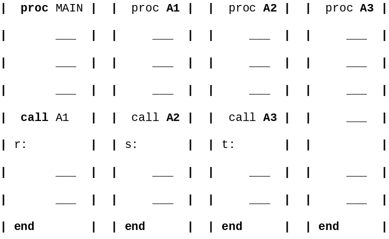
A complete SPARKS procedure has the form
procedure NAME (parameter list)
S
end
return (expr)
where the value of expr is delivered as the value of the procedure. The expr may be omitted in which case a return is made to the calling procedure. The
execution of an end at the end of procedure implies a return. A procedure may be invoked by using a call statement
call NAME (parameter list)
Procedures may call themselves, direct recursion, or there may be a sequence resulting in indirect recursion. Though recursion often carries with it a severe penalty at execution time, it remains all elegant way to describe many computing processes. This penalty will not deter us from using recursion. Many such
programs are easily translatable so that the recursion is removed and efficiency achieved.
A complete SPARKS program is a collection of one or more procedures, the first one taken as the main program. All procedures are treated as external, which means that the only means for communication between them is via parameters. This may be somewhat restrictive in practice, but for the purpose of exposition it helps to list all variables explicitly, as either local or parameter. The association of actual to formal parameters will be handled using the call by reference rule. This means that at run time the address of each parameter is passed to the called procedure. Parameters which are constants or values of expressions are stored into internally generated words whose addresses are then passed to the
procedure.
For input/output we assume the existence of two functions read (argument list), print (argument list)
Arguments may be variables or quoted strings. We avoid the problem of defining a "format" statement as we will need only the simplest form of input and output. The command stop halts execution of the currently executing procedure.
Comments may appear anywhere on a line enclosed by double slashes, e.g. //this is a comment//
lower and upper bounds. An n-dimensional array A with lower and upper bounds li, ui, 1 i n may be declared by using the syntax declareA(l1:u1, ...,ln:un). We have avoided introducing the record or structure concept. These are often useful features and when available they should be used. However, we will persist in building up a structure from the more elementary array concept.
Finally, we emphasize that all of our variables are assumed to be of type INTEGER unless stated otherwise.
Since most of the SPARKS programs will be read many more times than they will be executed, we have tried to make the code readable. This is a goal which should be aimed at by everyone who writes programs. The SPARKS language is rich enough so that one can create a good looking program by applying some simple rules of style.
(i) Every procedure should carefully specify its input and output variables. (ii) The meaning of variables should be defined.
(iii) The flow of the program should generally be forward except for normal looping or unavoidable instances.
(iv) Indentation rules should be established and followed so that computational units of program text can more easily be identified.
(v) Documentation should be short, but meaningful. Avoid sentences like ''i is increased by one."
(vi) Use subroutines where appropriate.
1.3 HOW TO CREATE PROGRAMS
Now that you have moved beyond the first course in computer science, you should be capable of developing your programs using something better than the seat-of-the-pants method. This method uses the philosophy: write something down and then try to get it working. Surprisingly, this method is in wide use today, with the result that an average programmer on an average job turns out only between five to ten lines of correct code per day. We hope your productivity will be greater. But to improve requires that you apply some discipline to the process of creating programs. To understand this process better, we consider it as broken up into five phases: requirements, design, analysis, coding, and
verification.
(i) Requirements. Make sure you understand the information you are given (the input) and what results you are to produce (the output). Try to write down a rigorous description of the input and output which covers all cases.
You are now ready to proceed to the design phase. Designing an algorithm is a task which can be done independently of the programming language you eventually plan to use. In fact, this is desirable because it means you can
postpone questions concerning how to represent your data and what a particular statement looks like and concentrate on the order of processing.
(ii) Design. You may have several data objects (such as a maze, a polynomial, or a list of names). For each object there will be some basic operations to perform on it (such as print the maze, add two polynomials, or find a name in the list). Assume that these operations already exist in the form of procedures and write an algorithm which solves the problem according to the requirements. Use a notation which is natural to the way you wish to describe the order of
processing.
(iii) Analysis. Can you think of another algorithm? If so, write it down. Next, try to compare these two methods. It may already be possible to tell if one will be more desirable than the other. If you can't distinguish between the two, choose one to work on for now and we will return to the second version later.
objects (a maze as a two dimensional array of zeros and ones, a polynomial as a one dimensional array of degree and coefficients, a list of names possibly as an array) and write algorithms for each of the operations on these objects. The order in which you do this may be crucial, because once you choose a representation, the resulting algorithms may be inefficient. Modern pedagogy suggests that all processing which is independent of the data representation be written out first. By postponing the choice of how the data is stored we can try to isolate what operations depend upon the choice of data representation. You should consider alternatives, note them down and review them later. Finally you produce a complete version of your first program.
It is often at this point that one realizes that a much better program could have been built. Perhaps you should have chosen the second design alternative or perhaps you have spoken to a friend who has done it better. This happens to industrial programmers as well. If you have been careful about keeping track of your previous work it may not be too difficult to make changes. One of the criteria of a good design is that it can absorb changes relatively easily. It is usually hard to decide whether to sacrifice this first attempt and begin again or just continue to get the first version working. Different situations call for
different decisions, but we suggest you eliminate the idea of working on both at the same time. If you do decide to scrap your work and begin again, you can take comfort in the fact that it will probably be easier the second time. In fact you may save as much debugging time later on by doing a new version now. This is a phenomenon which has been observed in practice.
The graph in figure 1.3 shows the time it took for the same group to build 3 FORTRAN compilers (A, B and C). For each compiler there is the time they estimated it would take them and the time it actually took. For each subsequent compiler their estimates became closer to the truth, but in every case they underestimated. Unwarrented optimism is a familiar disease in computing. But prior experience is definitely helpful and the time to build the third compiler was less than one fifth that for the first one.
Figure 1.3: History of three FORTRAN compilers
program you should attempt to prove it is correct. Proofs about programs are really no different from any other kinds of proofs, only the subject matter is different. If a correct proof can be obtained, then one is assured that for all
possible combinations of inputs, the program and its specification agree. Testing is the art of creating sample data upon which to run your program. If the
program fails to respond correctly then debugging is needed to determine what went wrong and how to correct it. One proof tells us more than any finite amount of testing, but proofs can be hard to obtain. Many times during the proving
process errors are discovered in the code. The proof can't be completed until these are changed. This is another use of program proving, namely as a
methodology for discovering errors. Finally there may be tools available at your computing center to aid in the testing process. One such tool instruments your source code and then tells you for every data set: (i) the number of times a statement was executed, (ii) the number of times a branch was taken, (iii) the smallest and largest values of all variables. As a minimal requirement, the test data you construct should force every statement to execute and every condition to assume the value true and false at least once.
One thing you have forgotten to do is to document. But why bother to document until the program is entirely finished and correct ? Because for each procedure you made some assumptions about its input and output. If you have written more than a few procedures, then you have already begun to forget what those
assumptions were. If you note them down with the code, the problem of getting the procedures to work together will be easier to solve. The larger the software, the more crucial is the need for documentation.
The previous discussion applies to the construction of a single procedure as well as to the writing of a large software system. Let us concentrate for a while on the question of developing a single procedure which solves a specific task. This shifts our emphasis away from the management and integration of the various procedures to the disciplined formulation of a single, reasonably small and well-defined task. The design process consists essentially of taking a proposed
approach. Inversely, the designer might choose to solve different parts of the problem directly in his programming language and then combine these pieces into a complete program. This is referred to as the bottom-up approach.
Experience suggests that the top-down approach should be followed when creating a program. However, in practice it is not necessary to unswervingly follow the method. A look ahead to problems which may arise later is often useful.
Underlying all of these strategies is the assumption that a language exists for adequately describing the processing of data at several abstract levels. For this purpose we use the language SPARKS coupled with carefully chosen English narrative. Such an algorithm might be called pseudo-SPARKS. Let us examine two examples of top-down program development.
Suppose we devise a program for sorting a set of n 1 distinct integers. One of the simplest solutions is given by the following
"from those integers which remain unsorted, find the smallest and place it next in the sorted list"
This statement is sufficient to construct a sorting program. However, several issues are not fully specified such as where and how the integers are initially stored and where the result is to be placed. One solution is to store the values in an array in such a way that the i-th integer is stored in the i-th array position, A(i)
Note how we have begun to use SPARKS pseudo-code. There now remain two clearly defined subtasks: (i) to find the minimum integer and (ii) to interchange it with A(i). This latter problem can be solved by the code
The first subtask can be solved by assuming the minimum is A (i), checking A(i) with A(i + 1), A(i + 2), ... and whenever a smaller element is found, regarding it as the new minimum. Eventually A(n) is compared to the current minimum and we are done. Putting all these observations together we get
procedure SORT(A,n) 1 for i 1 to n do
2 j i
3 for k j + 1 to n do
4 if A(k) < A(j) then j k
5 end
6 t A(i); A(i) A(j); A(j) t
7 end end SORT
The obvious question to ask at this point is: "does this program work correctly?" Theorem: Procedure SORT (A,n) correctly sorts a set of n 1 distinct integers, the result remains in A (1:n) such that A (1) < A (2) < ... < A(n).
Proof: We first note that for any i, say i = q, following the execution of lines 2 thru 6, it is the case that A(q) A(r), q < r n. Also, observe that when i
becomes greater than q, A(1 .. q) is unchanged. Hence, following the last execution of these lines, (i.e., i = n), we have A(1) A(2) ... A(n). We observe at this point that the upper limit of the for-loop in line 1 can be changed to n - 1 without damaging the correctness of the algorithm.
From the standpoint of readability we can ask if this program is good. Is there a more concise way of describing this algorithm which will still be as easy to comprehend? Substituting while statements for the for loops doesn't
language standard
IF (N. LE. 1) GO TO 100 NM1 = N - 1
DO 101 I = 1, NM1 J = I
JP1 = J + 1
DO 102 K = JP1, N
IF (A(K).LT.A(J)) J = K 102 CONTINUE
T = A(I) A(I) = A(J) A(J) = T 101 CONTINUE 100 CONTINUE
FORTRAN forces us to clutter up our algorithms with extra statements. The test for N = 1 is necessary because FORTRAN DO-LOOPS always insist on
executing once. Variables NM1 and JP1 are needed because of the restrictions on lower and upper limits of DO-LOOPS.
Let us develop another program. We assume that we have n 1 distinct integers which are already sorted and stored in the array A(1:n). Our task is to determine if the integer x is present and if so to return j such that x = A(j); otherwise return
j = 0. By making use of the fact that the set is sorted we conceive of the following efficient method:
upper, to indicate the range of elements not yet tested."
At this point you might try the method out on some sample numbers. This method is referred to as binary search. Note how at each stage the number of elements in the remaining set is decreased by about one half. We can now attempt a version using SPARKS pseudo code.
procedure BINSRCH(A,n,x,j)
initialize lower and upper
while there are more elements to check do
let A(mid) be the middle element
case
: x > A(mid): set lower to mid + 1
: x < A(mid): set upper to mid - 1 : else: found
end
end
not found
end BINSRCH
The above is not the only way we might write this program. For instance we could replace the while loop by a repeat-until statement with the same English condition. In fact there are at least six different binary search programs that can be produced which are all correct. There are many more that we might produce which would be incorrect. Part of the freedom comes from the initialization step. Whichever version we choose, we must be sure we understand the relationships between the variables. Below is one complete version.
procedure BINSRCH (A,n,x,j) 1 lower 1; upper n
3 mid (lower + upper) / 2 4 case
5 : x > A(mid): lower mid + 1 6 : x < A(mid): upper mid - 1 7 : else: j mid; return
8 end
9 end
10 j 0
end
To prove this program correct we make assertions about the relationship between variables before and after the while loop of steps 2-9. As we enter this loop and as long as x is not found the following holds:
lower upper andA (lower) x A (upper) and SORTED(A, n)
Now, if control passes out of the while loop past line 9 then we know the condition of line 2 is false
lower > upper.
This, combined with the above assertion implies that x is not present.
Recursion
We have tried to emphasize the need to structure a program to make it easier to achieve the goals of readability and correctness. Actually one of the most useful syntactical features for accomplishing this is the procedure. Given a set of
instructions which perform a logical operation, perhaps a very complex and long operation, they can be grouped together as a procedure. The procedure name and its parameters are viewed as a new instruction which can be used in other
programs. Given the input-output specifications of a procedure, we don't even have to know how the task is accomplished, only that it is available. This view of the procedure implies that it is invoked, executed and returns control to the appropriate place in the calling procedure. What this fails to stress is the fact that procedures may call themselves (direct recursion) before they are done or they may call other procedures which again invoke the calling procedure (indirect recursion). These recursive mechanisms are extremely powerful, but even more importantly, many times they can express an otherwise complex process very clearly. For these reasons we introduce recursion here.
Most students of computer science view recursion as a somewhat mystical technique which only is useful for some very special class of problems (such as computing factorials or Ackermann's function). This is unfortunate because any program that can be written using assignment, the if-then-else statement and the while statement can also be written using assignment, if-then-else and recursion. Of course, this does not say that the resulting program will necessarily be easier to understand. However, there are many instances when this will be the case. When is recursion an appropriate mechanism for algorithm exposition? One instance is when the problem itself is recursively defined. Factorial fits this category, also binomial coefficients where
can be recursively computed by the formula
Another example is reversing a character string, S = 'x1 ... xn' where SUBSTRING (S,i,j) is a function which returns the string xi ... xj for
strings (as in PL/I). Then the operation REVERSE is easily described recursively as
procedure REVERSE(S)
n LENGTH(S)
if n = 1 then return (S)
else return (REVERSE(SUBSTRING(S,2,n))
SUBSTRING(S,1,1))
end REVERSE
If this looks too simple let us develop a more complex recursive procedure. Given a set of n 1 elements the problem is to print all possible permutations of this set. For example if the set is {a,b,c}, then the set of permutations is {(a, b,c), (a,c,b), (b,a,c), (b,c,a), (c,a,b), (c,b,a)}. It is easy to see that given n
elements there are n ! different permutations. A simple algorithm can be achieved by looking at the case of four elements (a,b,c,d). The answer is obtained by printing
(i) a followed by all permutations of (b,c,d) (ii) b followed by all permutations of (a,c,d) (iii) c followed by all permutations of (b,a,d) (iv) d followed by all permutations of (b,c,a)
The expression "followed by all permutations" is the clue to recursion. It implies that we can solve the problem for a set with n elements if we had an algorithm which worked on n - 1 elements. These considerations lead to the following procedure which is invoked by call PERM(A,1,n). A is a character string e.g. A ='abcd', and INTERCHANGE (A,k,i) exchanges the k-th character of A with the i-th character of A.
procedure PERM(A,k,n)
B A
for i k to n do
call INTERCHANGE(A,k,i)
call PERM(A,k + 1,n) A B
end
end PERM
Try this algorithm out on sets of length one, two, and three to insure that you understand how it works. Then try to do one or more of the exercises at the end of this chapter which ask for recursive procedures.
Another time when recursion is useful is when the data structure that the
algorithm is to operate on is recursively defined. We will see several important examples of such structures, especially lists in section 4.9 and binary trees in section 5.4. Another instance when recursion is invaluable is when we want to describe a backtracking procedure. But for now we will content ourselves with examining some simple, iterative programs and show how to eliminate the iteration statements and replace them by recursion. This may sound strange, but the objective is not to show that the result is simpler to understand nor more efficient to execute. The main purpose is to make one more familiar with the execution of a recursive procedure.
Suppose we start with the sorting algorithm presented in this section. To rewrite it recursively the first thing we do is to remove the for loops and express the algorithm using assignment, if-then-else and the go-to statement.
procedure SORT(A,n)
i 1
Ll: if i n - 1 // for i 1 to n - 1 do//
L2: if k n //for k j + 1 to n do//
then [if A(k) < A(j)
then j k
k k + 1; go to L2]
t A(i); A(i) A(j); A(j) t i i + 1; go to L1]
end SORT
Now every place where we have a label we introduce a procedure whose parameters are the variables which are already assigned a value at that point. Every place where a ''go to label'' appears, we replace that statement by a call of the procedure associated with that label. This gives us the following set of three procedures.
procedure SORT(A,n)
call SORTL1(A,n,1)
end SORT
procedure SORTLl(A,n,i)
if i n - 1
then [j i; call MAXL2(A,n,j,i + 1)
t A(i); A(i) A(j); A(j) t
call SORTL1(A,n,i + 1)]
end SORTL1
procedure MAXL2(A,n,j,k)
then [if A(k) < A(j) then j k
call MAXL2(A,n,j,k + 1)]
end MAXL2
We can simplify these procedures somewhat by ignoring SORT(A,n) entirely and begin the sorting operation by call SORTL1(A,n,1). Notice how SORTL1 is directly recursive while it also uses procedure MAXL2. Procedure MAXL2 is also directly reculsive. These two procedures use eleven lines while the original iterative version was expressed in nine lines; not much of a difference. Notice how in MAXL2 the fourth parameter k is being changed. The effect of
increasing k by one and restarting the procedure has essentially the same effect as the for loop.
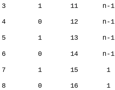
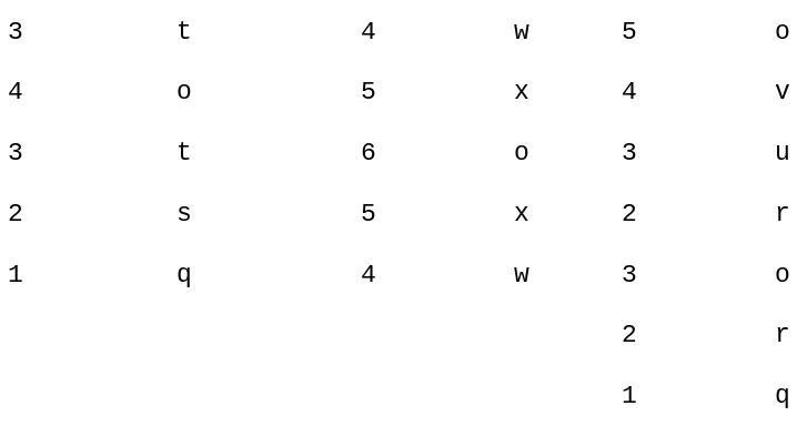
Now let us trace the action of these procedures as they sort a set of five integers
When a procedure is invoked an implicit branch to its beginning is made. Thus a recursive call of a program can be made to simulate a go to statement. The
parameter mechanism of the procedure is a form of assignment. Thus placing the argument k + 1 as the fourth parameter of MAXL2 is equivalent to the statement
k k + 1.
1.4 HOW TO ANALYZE
PROGRAMS
One goal of this book is to develop skills for making evaluative judgements about programs. There are many criteria upon which we can judge a program, for instance:
(i) Does it do what we want it to do?
(ii) Does it work correctly according to the original specifications of the task? (iii) Is there documentation which describes how to use it and how it works? (iv) Are subroutines created in such a way that they perform logical sub-functions?
(v) Is the code readable?
The above criteria are all vitally important when it comes to writing software, most especially for large systems. Though we will not be discussing how to reach these goals, we will try to achieve them throughout this book with the programs we write. Hopefully this more subtle approach will gradually infect your own program writing habits so that you will automatically strive to achieve these goals.
There are other criteria for judging programs which have a more direct
relationship to performance. These have to do with computing time and storage requirements of the algorithms. Performance evaluation can be loosely divided into 2 major phases: (a) a priori estimates and (b) a posteriori testing. Both of these are equally important.
First consider a priori estimation. Suppose that somewhere in one of your programs is the statement
We would like to determine two numbers for this statement. The first is the amount of time a single execution will take; the second is the number of times it is executed. The product of these numbers will be the total time taken by this statement. The second statistic is called the frequency count, and this may vary from data set to data set. One of the hardest tasks in estimating frequency counts is to choose adequate samples of data. It is impossible to determine exactly how much time it takes to execute any command unless we have the following
information:
(i) the machine we are executing on: (ii) its machine language instruction set;
(iii) the time required by each machine instruction;
(iv) the translation a compiler will make from the source to the machine language.
It is possible to determine these figures by choosing a real machine and an existing compiler. Another approach would be to define a hypothetical machine (with imaginary execution times), but make the times reasonably close to those of existing hardware so that resulting figures would be representative. Neither of these alternatives seems attractive. In both cases the exact times we would
determine would not apply to many machines or to any machine. Also, there would be the problem of the compiler, which could vary from machine to machine. Moreover, it is often difficult to get reliable timing figures because of clock limitations and a multi-programming or time sharing environment. Finally, the difficulty of learning another machine language outweighs the advantage of finding "exact" fictitious times. All these considerations lead us to limit our goals for an a priori analysis. Instead, we will concentrate on developing only the frequency count for all statements. The anomalies of machine configuration and language will be lumped together when we do our experimental studies. Parallelism will not be considered.
Consider the three examples of Figure 1.4 below.
. for i 1 to n do
. for j 1 to n do
x x + l x x + 1
. x x + 1 . end
. end end
(a) (b) (c) Figure 1.4: Three simple programs for frequency counting.
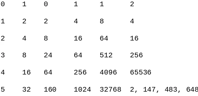
In program (a) we assume that the statement x x + 1 is not contained within any loop either explicit or implicit. Then its frequency count is one. In program (b) the same statement will be executed n times and in program (c) n2 times (assuming n 1). Now 1, n, and n2 are said to be different and increasing orders of magnitude just like 1, 10, 100 would be if we let n = 10. In our analysis of execution we will be concerned chiefly with determining the order of magnitude of an algorithm. This means determining those statements which may have the greatest frequency count.
To determine the order of magnitude, formulas such as
often occur. In the program segment of figure 1.4(c) the statement x x + 1 is executed
Simple forms for the above three formulas are well known, namely,
To clarify some of these ideas, let us look at a simple program for computing the
n-th Fibonacci number. The Fibonacci sequence starts as 0, 1, 1, 2, 3, 5, 8, 13, 21, 34, 55, ...
Each new term is obtained by taking the sum of the two previous terms. If we call the first term of the sequence F0 then F0 = 0, F1 = 1 and in general
Fn = Fn-1 + Fn-2, n 2.
The program on the following page takes any non-negative integer n and prints the value Fn.
1 procedure FIBONACCI
2 read (n)
3-4 if n < 0 then [print ('error'); stop] 5-6 if n = 0 then [print ('0'); stop] 7-8 if n = 1 then [print ('1'); stop] 9 fnm2 0; fnm 1 1
10 for i 2 to n do
11 fn fnm1 + fnm2 12 fnm2 fnm1
13 fnm1 fn
14 end
15 print (fn) 16 end FIBONACCI