Raffaella Bernardi
In this paper we look at the interpretation of Quantifier Phrases from the perspective of Symmetric Categorial Grammar. We show how the apparent mismatch between the syntactic and semantic behaviour of these expressions can be resolved in a typelogical system equipped with two Merge relations: one for syntactic units, and one for the evaluation contexts of the semantic values associated with these syntactic units.
Keywords: Symmetric Categorial Grammar, Terms and Contexts, Continuation Semantics, Quantifiers.
1
The Logic behind Natural Languages
“The Mathematics of Sentence Structures”, the title of (Lambek, 1958), clearly summarizes the ambitious challenge Jim Lambek has launched to researchers interested on formal approaches to natural language. It could also be read as asking “which is the logic that captures natural language composition?”, which can be rephrased as “which are the models of natural language composition?”, “which are its formal properties?”. Since (Montague, 1974), theλ-calculus was used by linguists to build the meaning representation of sentences compositionaly. The high expectations on the line of research pioneered by Lambek were even increased by Johan van Benthem’s results (van Benthem, 1987) on the correspondence between the iden-tified logic (known as Lambek calculus) and theλ-calculus. However, though all the questions above, and even more, were answered pretty soon (see (Lambek, 1961; Moortgat, 1988) among others), the an-swers found hold only for a fragment of natural language. What remains outside of the defined logic (and hence model and proof system) seemed to be those structures containing non-local dependencies and scope operators. The proof of the lack of expressivity of the Lambek calculus was given by the results on the correspondence of the proposed logics with Context Free Language, since it is known that natural language is out side this class of formal languages. Through the years, many proposals have been made to over-come these well defined limitations, but these proposals departed in a way or another from the original line of research Lambek had launched, e.g. they strive for wide coverage of the parser rather than for logical completeness of the system (Steedman, 2000).
In this paper, we go back to 1961 and start from there again, but with the new knowledge put at our disposal by research on algebra, logic, programming languages and linguistics. We show that the time is ready to recover the original enthusiasm on the possibility to solve Lambek’s original challenge. In particular, we focus on scope operators and the mismatch that they might create between syntactic and semantic structures. The original questions regarding the model, the proof systems, and the meaning representation of the structures recognized by the logic we will present are formally answered in (Kurtonina & Moortgat, 2007; Bernardi & Moortgat, 2007; Moortgat, 2007; Bernardi & Moortgat, 2009; Moortgat, 2009); here we give a more gentle introduction to the system we propose and focus on its contribution to the linguistic research on scope in natural language.
Lambek brought to the light the mathematical apparatus behind Categorial Grammar (CG) showing that CG was based on half of the residuation principle and illustrated the advantages that one would gain by considering the whole mathematical principle given below.
(RES) A⊆B/C iff A⊗C⊆B iff C⊆A\B
In more familiar term, the Lambek calculus, or calculus of residuation, consists of function application and abstraction rules, which are used to prove the grammaticality of a given sentence. For instance, given
thatAlexbelongs to the category of determiner phrases (dp) andleftto the one of intransitive verbs(dp\s) (i.e. a function missing adpon the left to yield a sentences), the expressionAlex leftis proved to belong to the categoryssimply by function application:
If Alex ∈ dp
left ∈ dp\s Then Alex left ∈ s
which is the proof of the following theorem:
(1) (a) dp⊗(dp\s)⊢s
While function application was already used in CG, Lambek showed that the residuation calculus in-cludes also abstraction which is needed, for instance, to prove the statement below, i.e. the type lifting rule used by linguists.
(2) (b) dp⊢s/(dp\s)
We propose to extend the expressivity of the logical grammar by moving to a symmetric calculus, i.e. a calculus in which each rule has a dual. The concept ofdual rulesanddual theoremswas introduced by Schr¨oder (Schr¨oder, 1980) who noticed that the rules of propositional logic could be formulated in pairs corresponding to De Morgan dual operators, e.g. the rules about∧are dual to rules about∨and so are the theorems below involving them:
A∧(B∨C)⊢(A∧B)∨(A∧C) dually (C∨A)∧(B∨A)⊢(C∧B)∨A
The logic language of the Lambek calculus consists of residuated operators ((A\B),(A⊗B),(B/A)). We extend it with their duals, viz. ((B⊘A),(B⊕A),(A;B)) and claim that besides the residuation principle (RES) the mathematics of sentence structures includes its dual principle (DRES),
(DRES) B⊘A⊆C iff B ⊆C⊕A iff C;B⊆A
together with the properties governing the interaction between residuated and dual residuated operators. These interaction properties were first studied by V. N. Grishin (Grishin, 1983). We call the new system Lambek Grishin (LG ) (See Section 3).
In the Lambek calculus the theorems dp⊗dp\s ⊢ sand dp ⊢ s/(dp\s) are proved by function application and abstraction, in the extended system also their duals hold:
(3) (a′) s⊢(s⊘dp)⊕dp (b′) (s⊘dp);s⊢dp
and are proved by co-application and co-abstraction, i.e. the dual rules of application and abstraction. In this new framework, we can distinguish categories standing for linguistic expressions and categories standing for the contexts of those expressions: contexts of categoryAare structures with anA-hole. The
⊗-relation merges linguistic expressions and the⊕-relation merges contexts where these expressions can be plugged in. For instance,dp\sstands forleftandknows mary, whereass⊘dpstands for the contexts of leftandknows mary, viz. the tree with a hole for that expression; for atomic formulas, we should distinguish between e.g.dp, standing formary, anddpcstanding for the context of adp. We can avoid marking this
difference at the level of atomic formulas since the merging relation used disambiguate them.
We briefly discuss the Quantifying In mechanism proposed in (Montague, 1974) and its variation, Quantifier Raising, proposed by linguists to describe the behavior of quantifiers (May, 1977; Reinhart, 1997) (Section 4). The logic obtained is in the Curry Howard Correspondence with theλµ¯ µ-calculus.e
The meaning representation of the parsed structures are built thanks to this correspondence. For reason of space, in this paper we won’t discuss this part; the reader interested in the issue is referred to (Bernardi & Moortgat, 2007, 2009); the only aspect to highlight here is that this extended lambda calculus has a way to represent and compose “context” too and to shift from one merging relation to the other.
between the Lambek calculus and its dual. The new framework sheds new lights that we believe could be of interest for other frameworks too:
1. besides having categories standing for words, there is the need of having categories standing for the words’ contexts;
2. hence, besides the merging relation, that builds a new syntactic unit from adjacent syntactic objects, natural language structures need also its dual relation, viz. the relation that merges contexts. (See (44) and (49) in Section 3.) Therefore, we can distinguish syntactic trees and context trees, the two types of trees can interact but their structure should not be modified once built. (See (51) in Section 3.)
3. non-local scope operators, like quantifiers, consist of a syntactic and a semantic component tied to each other. Thanks to the interaction between the two merging relations, the syntactic component stays in the syntactic structure or constituent-domain (c-domain) while the semantic component can jump out of it to reach the semantic-domain (s-domain), viz. the structure on which the QP has scope. (See (38) in Section 2 and Section 4.)
4. the c-domain is governed by the merging relation, whereas the s-domain is governed by the relation governing contexts. (See (62) and (74) in Section 4.)
5. a syntactic structure containing scope operators can be built in different ways: the order in which scope operators are activated determine the readings of the structure. (See (67), (71) in Section 4.)
2
Preliminary Background
Logic is about entailment of a conclusion from some premises. We might want to know whether it holds that whenever it is true thatIf Alex swims then Alex gets wet(p→q) and thatAlex swims(p) then it is also true thatAlex gets wet(q), which is formalized by the entailment below.
(4) {p→q, p} ⊢q
But as the objects of the reasoning vary, so it may vary the logic one needs. Our objects are natural language structures; hence we are interested in (a) tailoring the logic of natural language syntactic com-position and (b) capturing its correlation with the semantic representation. We want to grasp the fragment of logic that suits our needs, and use a logic as a grammar. This approach is known as the “parsing as deduction” approach.
Since the number and order of occurrence of formulas (words) and their structure are important when dealing with natural language the premise of our entailment is not a set as in propositional logic but a structure. In propositional logic, both{p→q, p, p} ⊢qand{p→(p→q), p} ⊢qhold, whereas we need a logic sensitive to the number and the order of the formulas.
As for (a), employing a logic as a grammar to analyse natural language expressions means to assign atomic or complex formulas to words and let their logical rules check that a given string of words is of a certain category and return its syntactic structure. Given the lexical entriesw1. . . wn, the system will
take the corresponding syntactic categoriesA1. . . Anand prove which structures they can receive so as to
derive a given categoryB, i.e., check whether a tree-structure of categoryB can be assigned to the given string of words.
(5) A1
|{z}
w1
· · · ·|{z}An wn
⊢B
To be more precise, syntactic categories are sets of expressions: those expressions that belong to a given category, i.e.dp\setc. are category labels: names for such sets. In short, we are dealing with e.g.:
{john, mary}
| {z }
np
×
|{z}
⊗
{left, knows lori
| {z }
np\s
} ⊆
|{z}
⊢
{john left, mary left, john knows lori, mary knows lori}
| {z }
We take the liberty to use the term “category” to refer to a category label. Similarly, the structure built out of the syntactic categories is a name for the sets of phrases that belong to that structure.
Since the introduction of theChomsky Hierarchy, the attention of formal linguists has focused on un-derstanding where natural languages fit in the hierarchy and hence, which formal grammars have the proper generative power to handle natural language structures. Similarly, when assuming a logical perspective the main question to address is which logic has the right expressivity to reason on natural language structures avoiding both under-generation and over-generation problems. In this perspective, the first question to ask is “which operators do we need to reason on natural language resources?”. Since Frege, the idea of in-terpreting words as functions and their composition as function application has been broadly accepted in Formal Semantics. Hence, implication (→) is an essential connective to have in our logical language. Yet, it remains to be understood which properties it should have, which other operators we would need and how they relate to each other.
A well known approach to our second goal (b) is the assumption of a Logical Form (Chomsky, 1976): the surface (syntactic) structure is input to a further set of rules which derive the Logical Form structure of the sentence. This latter structure is then interpreted by a semantic mechanism to obtain the meaning representation. Another well known solution is Montague’s (Montague, 1974) where syntax and seman-tics goes in parallel: for each syntactic rule there is a corresponding semantic rule that builds the mean-ing representation of the phrase analyzed syntactically. The correspondence is postulated for each rule. This step-by-step procedure in some intermediate steps, e.g. in the quantification step, may build meaning representations also for structures which are not syntactic constituents. Our approach is similar to Mon-tague’s in treating syntax and semantics in parallel, but it differs from it into two ways. A first important difference with Montague’s approach is that the correspondence between syntactic and semantic rules is defined at a general level: following (van Benthem, 1988), we exploit the correspondence introduced by Curry and Howard (Howard, 1980) between logical rules and lambda calculus; the proof of the derivation A1, . . . , An ⊢ B can be read as an instruction for the assembly of proof-termM with input parameters
x1, . . . , xn. In the “parsing as deduction” approach this turns out to mean thatlabelled derivationsprovide
also the schema to build the meaning representation of the structure under analysis:
(6) x1:|{z}A1
w1
· · · ·xn:|{z}An wn
⊢M :B
It’s important to emphasize that the correspondence holds between syntactic structures and semantic labels (proof terms). Recall the observation above that syntactic structures are labels for the set of expressions that belong to that structure. Once we instantiate the structure with a particular expression, we can also replace the semantic labels with the meaning representation of the words in the chosen expression. A second difference concerns the labelling of nodes: in LG only the syntactic constituents receive a semantic label.
Finally, there can be more than one way to prove that an entailment holds: different (normalized) derivations correspond to different readings of the same string of words. A given string can receive dif-ferent structures and difdif-ferent proof terms, but also difdif-ferent proof terms for the same structure. In this paper, we are interested in the latter case (see Section 4). For reason of space, we won’t discuss how a proof term is built by labelled derivations; however, since the linguistic phenomenon, we are interested in, lays on the interface of syntax and semantics of natural language, we introduce those concepts of Formal Semantics that are going to play a role in our analysis of quantifier phrases. The interested reader is referred to (van Benthem, 1987) for an introduction to the use of labelled derivations for building meaning represen-tation of parsed strings, and to (Bernardi & Moortgat, 2007, 2009) for the discussion of the Curry-Howard correspondence for the logic presented in this paper withλµ¯ µ-calculus and its translation intoe λ-terms.
2.1
Syntax-Semantics interface in Natural Language
E={lori,alex,sara,pim}; let[[w]]indicate the interpretation ofw.
(7) [[lori]] = lori;
[[alex]] = alex;
[[sara]] = sara;
[[pim]] = pim;
[[student]] = {alex, sara, lori};
[[teacher]] = {pim};
[[sing]] = {alex, sara, lori, pim};
[[trust]] = {halex, alexi};
[[know]] = {hlori, alexi,hlori, saraihlori, lorii};
[[left]] = {lori};
[[every student]] = {Y ⊆E|[[student]]⊆Y}.
This amounts to saying that, for example, the relation knowis theset of pairshα, βiwhere “αknows β”; or thatstudentis the set of all those elements which are a student. The case ofevery studentis more interesting: it denotes the set of properties that every student has.
(8) [[every student]] ={Y ⊆E|[[student]]⊆Y} = {{alex, sara, lori},{alex, sara, lori, pim}} = {[[student]],[[sing]]}
Alternatively, the words above can be seen as functions from the elements of their set to truth values. For instance, an intransitive verb likeleftcan be seen as a function that, given an entityeas argument, will return a truth valuet(left(lori)= true,left(alex)= false). The standard way of representing functions is by means of lambda terms: each word can be assigned a lambda term representing its meaning. For instance, a transitive verb like,knowsortrust, is represented as a function with two arguments (or a function taking the ordered pair of the element in the sets above). To see expressions as functions allows to consider natural language expressions as built by means of function application. Richard Montague introduced the idea that the step that put together the syntactic structure are associated with the ones that give instructions for assembling meaning representations: the syntactic and semantic rules in his grammar work in parallel. Here, we introduce those concepts of Montague Grammar that are essential for the understanding of our proposal, namely Categorial Grammar and the connection between syntax and semantics.
Syntax-Semantics In Categorial Grammar (CG) syntactic categories can be atomic or complex. The
latter are assigned to those expressions that are interpreted as functions and are designed to distinguish whether the argumentAmust occur to the left (A\B) or the right (B/A) of the function. Hence, function application comes in two versions, a Forward Application (FA) and a Backward Application (BA):
(9) (FA) B
B/A A
(BA) B
A A\B
The possibility to express whether the argument must occur on the left or the right of the function is important, for instance, in the case of the two arguments taken by the transitive verb: In English the object occurs on its right and the subject on its left. Having in mind the observation made above, viz. that a category is a name for the set of expressions that belong to it, we can look at function application in more precise terms. Given the categoriesA, B, CandDsuch thatC ⊆AandB ⊆D, i.e. every expression in Cis also inAand every expression inB is also inD, then if a functor category combines with elements ofA as an argument (i.e. it’s eitherA\·or ·/A), it also combines with elements ofC; the result of the application is an expression that belongs to the setB and hence to anyDof whichBis a subset. We will come back to this observation when looking at the dual Lambek Calculus in Section 3.
(10) (FA) B⊆D
B/A C⊆A
(BA) B ⊆D
word category type λ-term meaning
alex dp e alex alex
left dp\s e→t λxe.(leftx)t {lori}
trusts (dp\s)/dp e→(e→t) λxe.(λye.((trustsx)y)t) {halex, alexi}
student n e→t λxe.(studentx)t {alex, sara, lori}
every student (s/dp)\s (e→t)→t λY.∀λx.((studentx)⇒(Y x)) {Y ⊆E|[[student]]⊆Y}
Table 1: Syntactic categories and Semantic types
The whole picture of our little lexicon is summarized in Table 1, where for each word is given the syntactic categorial category, its corresponding semantic type as well as the lambda term of that type that represents the set theoretical meaning of the word given in the last column of the table. We indicate only one representative for each category.1,2
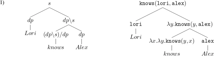
We can now look at an example highlighting the syntax-semantics link captured by CG and its connec-tion with theλ-calculus. The syntactic tree (tree on the left) is built by (FA) and (BA) and each step in it has a one-to-one correspondence with theλ-rules applied to assemble the semantic representation (the tree on the right).
(11) s
dp
Lori
dp\s
(dp\s)/dp
knows
dp
Alex
knows(lori,alex)
lori
Lori
λy.knows(y,alex)
λx.λy.knows(y, x)
knows
alex
Alex
2.2
The Mathematics of Sentence Structure (Lambek ’58 and ’61)
Lambek (Lambek, 1958) showed that the deduction theorem, that is the backbone of Logic, is also at the heart of linguistic structure composition. With this application in mind, the theorem says that if a linguistic structureΓcomposed with another constituent of syntactic categoryAis of categoryBthenΓis of category BgivenA, or alternatively, it is aBmissing aA
(12) If A,Γ⊢B then Γ⊢A→B
For instance, ifLori knows the studentis a sentence thenknows the studentis a sentence missing a deter-miner phrase –given thatLoriis of the latter category (dp).
(13) If Loridp,[knows the student]⊢s then [knows the student]⊢dp→s
The connection above between the comma and the implication is known in algebra as residuation principle and it’s an “iff”. This principle is also behind the more familiar mathematical operators of multiplication (×) and division (−):
(14) x×y≤z iff y≤ z
x
The reader can compare the similar behaviour shown by the×and−with respect to the≤with the one of the , and→ with the ⊢. To learn from this comparison, one can observe that the multiplication is characterized by some well known properties like commutativity, associativity and distributivity over the
+:
Similarly, we are interested in knowing which are the properties of the “comma” above when the con-catenated elements are words. In the approach we follow, the “comma” is taken to be not-commutative and not-associative to avoid over-generation problems. (For other choices, see (Steedman, 2000), among others).
As the comma’s behavior varies, so does the conditional’s. In particular, when rejecting commutativity of the comma the implication splits into left implication (A\B, “ifAon the left thenB”) and right impli-cation (B/A, “B ifAon the right”), since the order of occurrences of the formulas matters. Hence, the residuation principle becomes:
(16)
(a1) A⊗C⊢B iff C⊢A\B
(a2) C⊗A⊢B iff C⊢B/A
The difference with the comma is emphasised by using the⊗operator in its place.
NL (Non-associative Lambek calculus), introduced in (Lambek, 1961), is the pure calculus of residua-tion since it is characterized by only these two rules (besides transitivity, viz., ifA ⊢BandB ⊢C, then A⊢C, and reflexivity, viz.A⊢A, of the⊢).
As we have observed when introducing CG, distinguishing the left and right implication turns out to be relevant when formulas stand for syntactic categories of words. By applying the residuation principle we obtain the category of a verb phrase as well as the one of a transitive verb.
(17)
(a1) Loridp⊗[knows the student]⊢s iff [knows the student]⊢dp\s
(a2) [knows]tv⊗[the student]dp⊢dp\s iff [knows]tv ⊢(dp\s)/dp
Furthermore, the object of our toy example is adpconsisting of a noun (student) that is assigned the atomic categorynand an article (the). Its category is determined in the, by now, usual way:
[the]⊗[student]n⊢dp iff [the]⊢dp/n
Forward and Backward function applications are theorems of this calculus:
(18) B/A⊗A⊢B and A⊗A\B⊢B
The Lambek Calculus is the logic of themergingrelation represented by the⊗(See (Vermaat, 2005) for a detailed comparison of this relation with the Merge relation of the Minimalist Framework):
(19) If there are two expressionse1 ∈ B/A, e2 ∈ As.t. Merge(e1, e2, e3), i.e. e3 is the result
of merging e1ande2, then by definition of⊗, e3 ∈ B/A⊗A, and, hencee3 ∈ B, since
B/A⊗A ⊢ B. An expressione1belongs to a functor categoryB/Aiffor allexpressions
e2, e3such thatMerge(e1, e2, e3)ande2∈A, thene3∈B.
2.3
“Parsing as Deduction”: Sequent Calculus
A logic can be presented in several proof-system styles. Natural Deduction is the most well known one among linguists familiar with Logic. Other systems are Gentzen Sequent Calculus, Tableaux, Proof nets. Here we will use Sequent Calculus since it is the most suitable for introducing the concept of dual proofs and symmetric calculus that are at the heart of our proposal. It is a “decision procedure” and we use it to determine whether a phrase is a well-formed expression of a given category (and to assign it a meaning representation in the process of checking this.)
Gentzen Sequents Sequent Calculus is a proof system introduced by Gentzen to reason on structures. A
sequenthas the form
where bothΣandΓare sequences of logical formulas (i.e., both the number and the order of the occurring formula matter). The symbol⊢ is usually referred to as turnstile and is often read, suggestively, as “yields” or “proves”; it is not a symbol in the language, rather it is a symbol in the metalanguage used to discuss proofs. In the sequent above,Σis called the antecedent andΓis said to be the succedent of the sequent. A sequent derivation starts from the sequent to be proved and by application of the inference rules reduces it into simpler sequents (roughly, a sequent with a lower number of operators). In other words, inference rules are precise instructions to build the derivation of a given sequent. The choice of which inference rule to apply is dictated by the main operators of the formulas in the sequent. As we will show later, in same cases more choices are possible. A derivation is concluded when axiom links are reached.
The properties of the calculus determines the actual inference rules which are written with a list of se-quents above (premises) and below a line (conclusion). Each operator has an inference rule that eliminates it from the left of the turnstile and an inference rule that eliminates it from the right.3 For instance, the logical rule that eliminates∧of propositional logic from the left of the turnstile is represented as following
(21)
Γ[A]⊢∆
Γ[A∧B]⊢∆ (∧L)
The rule says: the structureΓcontaining the formulaA∧Byields the structure∆, ifΓcontainingA can be proved to yield∆, i.e. the problem of proving the sequent in the conclusion is reduced to a simpler problem by eliminating the∧.
Non-associative Lambek Calculus In the case of the Non-associative Lambek calculus (NL ) the property
encoded into the inference rules is the residuation principle discussed above. Here we do not go into the details of how this principle is captured by the inference rules of the Sequent proof system, and refer the reader interested in the issue to (Areces & Bernardi, 2004). Since in NL the sequence can be seen as tree-structure, to help understanding the austere sequent notation for each inference rule of the calculus we give a tree representation as well. In NL the succedent of sequents is not a structure but a formula:
(22)
Σ⊢A
∑
•
A
This statement expresses the judgement that the tree structureΣis of categoryA. Thinking of categories as labels for sets of expressions, the sequent can be read as a proof of the fact that every expression inΣis also inA. We will thus take the liberty of saying that the sequent proves that the structureΣis of category A.
Recall, that trees are bracketed strings of formulas. The smallest tree is just a single formulaA. Com-posite trees are formed by taking two treesΓand∆together as immediate daughters of a binary branching structure. In the sequent notation, we write(Γ,∆). Graphically,
•
•
x x x x x
x •
GGG GGGG
Γ ∆
)) ) ))
)) ))
** **
** **
**
A
•
A
where we write the formula at the left-hand side of⊢below the node•, and the formula at the right-hand side above it.
The axiom case deals with the simplest possible trees — trees consisting of one single formula. Next we need rules to reason about composite trees. Consider first the situation where we have a treeΓwhich has among its leaves a formulaB. Suppose we have arrived at the judgment that this tree is of categoryC. We can graphically depict this situation as
C • Γ • ** ** ** *** B
In the language of sequent calculus we writeΓ[B] ⊢ C. The square bracket notationΓ[Γ′]is used for picking out a distinguished sub-treeΓ′in a treeΓ. In this particular case, the sub-treeΓ′is the single-node treeB.
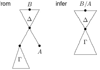
Suppose now that we also have a second tree∆which we can show to be of categoryB. In that case, substituting the tree∆for the nodeBinΓwill produce a tree that is still of categoryC. In other words: in a well-formed phrase of categoryC, we can replace any of its constituents by another constituent, as long as the replacement and the original constituent has the same category.
This grammaticality-preserving substitution yields the inference rule below, which is known as the Cut rule. from B • ∆ ** ** ** ** ** and C • Γ • ** ** ** *** B infer C • Γ • ** ** ** *** ∆ ** ** ** ***
In the concise sequent notation, we write4
∆⊢B Γ[B]⊢C
Γ[∆]⊢C (Cut)
Logical rules: The Axiom and the Cut rule do not mention particular category-forming operations: they hold in full generality for any formula. Let us turn then to the inference rules for the category-forming operations. For each of the connectives of our grammar logic,/,⊗,\, we need a rule that tells us how to deal with it when we find it right of the derivability sign⊢, or left of it. The first kind of rules are called rules of proof: they tell us how to arrive at a judgementΓ⊢Bin the case whereBis a complex formula: B/A,A\B, orA⊗B. The rules for the connectives left of⊢are calledrules of use: they tell us how we can put the treeΓtogether in accordance with the interpretation of the connectives/,⊗,\.
• • | | | | | | • 7777 7 B/A A
More generally (and using our substitution reasoning again), we obtain a tree of categoryBby com-biningB/Awith any sister tree∆on its right, provided we can show∆is of categoryA. Putting these steps together, we obtain the(/L)inference rule, introducing/in the antecedent tree structure.
from A • ∆ ** ** ** ** ** and C • Γ • ** ** ** *** B infer C • Γ • 11 11 11 11 11 • y y y y y y • GGGGGG G B/A ∆ && && && && && &
In sequent notation, we have:
∆⊢A
A⊢A B⊢B
B/A⊗A⊢B (/L) Γ[B]⊢C
Γ[B/A⊗A]⊢C (Cut)
Γ[B/A⊗∆]⊢C (Cut)
In other words, the function application rule can be applied within a tree and its compact formulation is as below.
(23)
∆⊢A Γ[B]⊢C
Γ[B/A⊗∆]⊢C (/L)
B
•
If A and C
Γ ∆ Γ ∆ • • B/A C
The elimination of the/from the left of the turnstile,(/L), is the application of a function of category B/Ato a structure∆, i.e. the sub-structureB/A⊗∆is proved to be of categoryB, if∆can be proved to be of categoryA. The application happens within a bigger structureΓ. Therefore, the sequent is reduced into two simpler sequents. In particular, in the premise in the right branch the sub-structureB/A⊗∆is replaced by its categoryB. In other words, the sequent in the conclusion holds if it can be proved that∆
yieldsAand the structureΓcontainingByieldsC. Notice that ifΓis a structure consisting only ofB/A and∆, then the right branch isB⊢C. Similarly for theA\Bcase.
the(/L)rule. We check, in other words, whether the transitive verb(dp2\s1)/dp3 indeed has a tree of
categorydpas its right sister. The atomic treedp4for the direct objectAlexqualifies. What remains to be
shown is that the subject verb-phrase combination(dp1,(dp2\s1))is indeed a tree of categorys.
(/L) s2
• • l l l l l l l l l l • PPPP PPPPP dp1 • { { { { { { { { { { { • 00 00 00 00
(dp2\s1)/dp3 dp4
if dp3
•
dp4
and s2
• • y y y y y y • NNNN NNNN dp1 (dp2\s1)
This is shown by applying the(\L)rule.
(\L) s2
• • y y y y y y • NNNN NNNN dp1 (dp2\s1)
if dp2
•
dp1
and s2 •
s1
This rather laborious graphical account of the derivation can be written down more compactly in the sequent notation:
dp4⊢dp3
dp1⊢dp2 s1⊢s2 (dp1,(dp2\s1))⊢s2
(\L)
(dp1
|{z}
[Lori
,(((dp2\s1)/dp3)
| {z }
[knows
, dp4
|{z}
Alex]]
))⊢s2 (/L)
The(/L)and(\L)rules provide instructions on how to use formulasB/A,A\B to build tree struc-tures. In sum, by application of inference rules, i.e. by structure simplification, we have reduced the whole structuredp1⊗((dp2\s1)/dp3⊗dp4)tos1which matches the top formulas2(s1 ⊢ s2). In the tree we
represent this match between thes-categories since it will play a role in the description of the QP analysis:
(24) s1⊢s2
dp1
|{z}
Lori (|dp2\s{z1)/dp3} knows
dp4
|{z}
Alex
Let us turn then to the rules that tell us how we can decide that a tree structureΓis of categoryB/A orA\B. Given the interpretation of the slashes, this will be the case ifΓtogether with a sister nodeAto its right or left, can be shown to be a tree of categoryB. For formulasB/A, we obtain the(/R)inference rule below. from B • • • ;; ;;; A Γ )) )) )) )) ))) infer B/A • Γ ,, ,, ,, ,, ,,
(Γ, A)⊢B
Γ⊢B/A (/R)
(A,Γ)⊢B
Γ⊢A\B (\R)
An interesting use of the right rules is the theoremA ⊢ C/(A\C), an instance of which is the type lifting rule known to linguists, viz. frometo(e→ t) →t. Any word of categorydpis proved to be of categorys/(dp\s). In other words, any expression that is in the category of determiner phrases is also in the category of quantifier phrases; any expression that is interpreted as an entity can be interpreted as the set of its properties (compare Table 1).
(25)
dp1⊢dp2 s2⊢s1
dp1⊗dp2\s2⊢s1 (\L)
dp1⊢s1/(dp2\s2)
(/R) dp1
s1/(d2\s2)
dp1 dp2\s2 s1
dp1 dp2
s2 s1
If If • and •
•
•
Since in the sequent in the conclusion there is only one main operator,/, and it occurs on the right of the turnstile, the only rule that can be applied is (/R), hence the sequent is reduced to a simpler sequent (a sequent with less implication operators), viz. dp1⊗dp2\s2 ⊢ s1. This sequent holds if dp1 ⊢ dp2
ands2 ⊢ s1, since both are axioms we are done. Notice thats/(dp\s)6⊢ dp, as one would expected by
thinking of the domains of interpretation of the corresponding functions, viz. it is not true that whatever can be interpreted as a set of properties can be interpreted as an entity.
This theorem is an essential part of the proofs of “Argument Lowering”, B/(C/(A\C)) ⊢ B/A, and “Value Raising”,B/A ⊢ (C/(B\C))/A, used by Hendriks (Hendriks, 1993) to account for scope ambiguities. We give the sequent derivation, the reader is invited to translate them into a tree notation.
(26) ....
A⊢C/(A\C) B ⊢B B/(C/(A\C))⊗A⊢B (/L)
B/(C/(A\C))⊢B/A (/R)
A⊢A
.. .. B⊢C/(B\C)
B/A⊗A⊢(C/(B\C)) (/L)
B/A⊢(C/(B\C))/A (/R)
Hendriks uses also a third rule called “Argument Raising”: this rule is not a theorem of the Logic, since as we have mentioned aboveC/(A\C)does not deriveAand hence the proof fails to reach all axioms.5 (See (Bastenhof, 2007) for a detailed discussion on Argument Raising.)
FAILED .. ..
C/(A\C)⊢A A⊢A B/A⊗C/(A\C)⊢B (/L) B/A⊢B/(C/(A\C)) (/R)
Bottom-up vs. Top-down parsing strategies Let us now consider the sentenceThe student who knows
Sara left. The relative pronounwhoworks as a bridge between a sentence missing adpin subject position, knows Sara, and the nounstudentthat the relative clause modifies, viz.who∈ (n\n)/(dp\s)as we can compute by means of the residuation principle:
(27)
[who]rel⊗[knows Sara]dp\s⊢n\n iff [who]rel⊢(n\n)/(dp\s)
This example will help us bringing in another important observation regarding parsing strategies. In the examples seen so far, at each step there was only one possible inference rule that could have been applied. However, it can happen that a sequent could be proved in more than one way. For instance, it contains more than one complex formula either in the antecedent or the succedent position. One can choose to follow either a (i) bottom-up or a (ii) top-down strategy as we will illustrate with the example below.
(28)
(n\n)/(dp\s)
| {z }
who (|dp\{zs)/dp}
knows
dp
|{z}
Sara
At each inference step, we follow a bottom-up strategies: We start from the bottom of the tree. In the leaves, there are two complex formulas that could be activated, hence there are two possible inference rules to apply as a first step: we could simplify the sequent either (i) by applying the function(dp2\s2)/dp3to
dp4or (ii) by applying the function(n\n)/(dp\s)to the sub-structure((dp2\s)/dp3⊗dp4). In a
bottom-up approach the choice is guided by the atomic categories in the leaves, hence, in this case bydp4. The
function to activate first is, therefore, the one of the transitive verb whose argument matches the atomic leave. The other inference steps are applied using these same criteria. In the tree notation, we leave the last two trees unfolded. The reader can check by herself the last steps that lead to the axiom links indicated in the sequent.
(29) Bottom-up strategy:
dp4⊢dp3
dp1⊢dp2 s2⊢s1
dp1⊗dp2\s2⊢s1 (\L)
dp2\s2⊢dp1\s1 (\R)
n3⊢n1 n2⊢n4
n3⊗n1\n2⊢n4 (\L)
n1\n2⊢n3\n4 (\R)
(n1\n2)/(dp1\s1)⊗dp2\s2⊢n3\n4
(/L)
(n1\n2)/(dp1\s1)
| {z }
[who
⊗((dp2\s2)/dp3
| {z }
[knows
⊗ dp4
|{z}
Sara]]
)⊢n3\n4 (/L)
If dp4 dp3 and (n1\n2)/(dp1\s1) dp2\s2 n3\n4 if dp2\s2 dp1\s1 and n1\n2 n3\n4 • • • •
The top-down strategy is illustrated below both in the sequent and in the tree notation. The starting point is the top-formulan3\n4, that can be simplified by(\R). The next step is the inference rules whose
result matches the new top formula, i.e.n4. Hence, the function activated first is the category of who.
Again we leave to the reader the unfolding of the last trees into the axiom links.
(30) Top-down strategy:
dp4⊢dp3
dp1⊢dp2 s2⊢s1
dp1⊗dp2\s2⊢s1 (\L)
dp2\s2⊢dp1\s1 (\R)
(dp2\s2)/dp3⊗dp4⊢dp1\s1
(/L) n3⊢n1 n2⊢n4
n3⊗n1\n2⊢n4 (\R)
n3⊗((n1\n2)/(dp1\s1)⊗((dp2\s2)/dp3⊗dp4))⊢n4 (/L)
(n1\n2)/(dp1\s1)
| {z }
[who
⊗((dp2\s2)/dp3
| {z }
[knows
⊗ dp4
|{z}
Sara]]
)⊢n3\n4 (\R)
(n1\n2)/(dp1\s1) n4
(dp2\s2)/dp3 dp4
if dp1\s1 and n4
n3 n1\n2 If
• •
The first toy example shows that NL captures the composition principle involved in kernel sentences —sentences consisting of local dependencies only (dependencies among juxtaposed constituents). It also illustrates how the concepts of dependency and constituent, so important when looking at natural language, are encoded in the derivation. The dependency between the verb and its arguments are captured by the axiom links involving the determiner phrases, on the other hand the brackets put around the structure at each step in the derivation build the constituents out of the single words. The last example shows that NL also properly handles extraction when it happens from a peripheral (accessible) position.
2.4
Lambek Calculus limitations
Since in NL function application can happen only on juxtaposed structures, abstraction only from periph-eral position, and there is no way of re-bracketing the tree once built. As a consequence, the system fails to recognize long distance dependencies and cross-dependencies, and does not capture the behavior of in-situ binders, like natural language quantifiers. Let’s look at their case now.
An important concept to introduce regards the notion of “scope” of quantifiers. Like in logic, the scope of a quantifier is the part of the expression on which it performs its action; the quantifier binds the variable xof categorydpin its scope, e.g. the action of∀below is to check all the possible assignments of values to the variablexit binds.
(31) s
s/(dp\s)
| {z }
everyone
dp\s
(dp\s)/dp
| {z }
knows
dp |{z}
Lori
∀λz.(knows(z,lori))
λY.∀λz.(Y z) λx.knows(x,lori)
λy.λx.knows(x, y) Lori
The category that we have shown to be derivable fromdpand that is mapped into the semantic type
(e→t)→tworks properly in NL when in subject position. However, this category does not capture the behaviour of QP in general, e.g. it already causes a failure of the proof when assigned to a QP in object position, as marked by the question marks in the syntactic tree.
(32)
s4
dp1
|{z}
Lori
??
(dp2\s1)/dp3
| {z }
knows
(s2/dp4)\s3
| {z }
everyone
∀λz.(knows(lori, z))
λx.knows(lori, x)
knows(lori, x)
lori λz.knows(z, x)
λy.λz.knows(z, y) x
λY.∀λz.(Y z)
NL is not expressive enough to account for this behaviour of QP. Our goal is to understand which are the formal properties that characterize this behaviour.
If one wants to mimic the semantic tree at the syntactic level, she could assign to QPs a second category,
(s/dp)\sthat is also mapped into(e→t)→tand would need to be able to obtain the following tree on the left, which by function application is reduced to the two simpler trees on the right:
(33)
s4
dp1
|{z}
Lori
(dp2\s1)/dp3
| {z }
knows
(s2/dp4)\s3
| {z }
everyone
If s2/dp4
dp1
|{z}
Lori
(dp2\s1)/dp3
| {z }
knows
and s4 •
s3
This can be proved by abstraction
(34)
s2/dp4
dp1
|{z}
Lori
(dp2\s1)/dp3
| {z }
knows
If s2
dp1
|{z}
Lori
(dp2\s1)/dp3
| {z }
knows
dp4
We have arrived to a tree that cannot be simplified further by means of the Lambek calculus’ inference rules. One would first need to re-bracket it,
(35)
s2
dp1
|{z}
Lori (|dp2\s{z1)/dp3} knows
dp4
The tree obtained can then be simplified by function applications, arriving at the following matches of atomic formulas:
(36)
dp2 •
dp1
dp3 •
dp4
s2 •
s1
The re-bracketing corresponds to applying the associativity rule as shown in the sequent below where the corresponding inference step is marked by (Ass); the reader can check the correspondence of each inference rule with the above trees.
(37)
dp1⊢dp2 dp4⊢dp3 s1⊢s2
.. .. D..
..
dp1⊗((dp2\s1)/dp3⊗dp4)⊢s2 (dp1⊗(dp2\s1)/dp3)⊗dp4⊢s2
(Ass)
dp1⊗(dp2\s1)/dp2⊢s2/dp4 (/R)
s3⊢s4 (dp1
|{z}
[Lori
⊗((dp2\s1)/dp2
| {z }
[knows
⊗(s2/dp4)\s3
| {z }
everyone]]
The derivation above proves that the structure [Lori [knows everyone]] belongs tos4. However, adding
associativity (Ass) to NL , i.e. going back to the Lambek’s ’58 paper, and using two different categories for quantifier in subject and object position is still not a general solution: the QP won’t be able to jump out from any position, but only from those that can become peripheral by associativity, e.g [Lori [thinks [Alice read a book ] while she was ill ] ] would receive only one reading.
Still it is interesting to reflect on the two examples with QP in subject and object position to grasp proof-theoretical insights on the syntax-semantic interface of natural language structures involving scope operators.
Syntax-Semantics seen from the axiom links The above example suggests that we can read the scope of
the functions in the parsed structure out of the axiom links of thes-atomic formulas: the fact thatEveryone has scope over the whole-structure (has wide scope) is captured by the axiom links3 ⊢ s4; the fact that
the transitive verb is in the immediate scope of the quantifier is captured by the the axiom links1 ⊢ s2.
Furthermore, the fact that the quantifier binds the variable taken as object by the transitive verb is captured by the axiom linkdp4⊢dp3.
We can elaborate further what we have just observed by saying that a quantifier could intuitively be considered as consisting of two components tied to each other: adpand a function that takes the sentential domain to produce a sentence. The syntactic component (dp) should stay in the embedded position where it works as argument of a verb, and the scope component should be free to travel through the tree so to reach its top level, without modifying the constituent structure. Below we focus on the scope component and represent it schematically assval/sarg(compare(sarg/dp)\svalandsval/(dp\sarg)).6 Generalizing,
we consider a structure with two scope-operators (OP1, OP2) and give the two possible scoping order
possibilities.
(38)
sval1⊢sgoal
OP1: sval1/sarg1 sval2⊢sarg1
OP2: sval2/sarg2 s⊢sarg2
dp2. . . dp1
sval2⊢sgoal
OP2: sval2/sarg2 sval1 ⊢sarg2
OP1: sval1/sarg1 s⊢sarg1
dp2. . . dp1
The trees are consistent with the standard idea that the later a quantifier is introduced in the semantic structure the wider its scope. In Section 4, we discuss the formal properties that characterize the function sval/sargand its connection with thedpcomponent as well as the composition relation holding between it
and the structure over which it takes scope.
In short, the QP category that can be assigned using residuated operators gives raise to the following problems: (i) it requires multiple category assignments for the QP in subject and object position; it fails to produce both (ii) local and (iii) non-local scope ambiguity. We show that using dual residuated operators, QP can be assigned one category that overcomes these three problems. Reasoning with natural language structure requires some categories tojump outof the structure where they sit leaving, however, the structure of the other components unchanged. We show that this ability is captured by the calculus consisting of residuation, dual residuation and the distributivity principles.
3
“The Mathematics of Sentence Structure” Revised
The reader may recall the De Morgan’s laws, i.e. rules relating pairs of dual logical operators in a systematic manner expressed in terms of negation. For instance,
(39) ¬(A∧B) =¬A∨ ¬B
which in words says: Since it is false that two things together are true, at least one of them must be false. Saying that this equality holds for propositional logic means that ¬(A∧B) ⊢ ¬A∨ ¬B and
¬A∨ ¬B⊢ ¬(A∧B)are theorems of the Logic.
In (Schr¨oder, 1980) it is introduced the concept of dual rules, for instance, the two rules below are duals. Their duality is expressed in terms of the sequent-turnstile, the two rules are perfectly symmetric with respect to the turnstile:
(40)
Γ[A]⊢∆
Γ[A∧B]⊢∆ (∧L) dually
Γ⊢∆[A]
Γ⊢∆[B∨A] (∨R).
Similarly, one can think of dual theorems. For instance, one could express either the distributivity of the∧over the∨or dually the one of the∨over the∧.
(41)
A∧(B∨C)⊢(A∧B)∨(A∧C) dually (C∨A)∧(B∨A)⊢(C∧B)∨A;
(A∧B)∨(A∧C)⊢A∧(B∨C) dually (C∧B)∨A⊢(C∨A)∧(B∨A).
¬is one of the logical operators of propositional logic, whereas it is not part of the logical language of the Lambek calculus. Hence, we cannot define duality in De Morgan’s style at the object-language level. However, we can still define it at the meta-level in terms of the behaviour of the operators w.r.t. the turnstile.
Residuation and Dual Residuation The logical operators of the Lambek Calculus are(\,⊗, /); we
in-troduce new operators(⊘,⊕,;)and define them as duals of the former in terms of their behaviour with respect to the⊢. The dual residuation principle was studied by V. N. Grishin (Grishin, 1983) and further investigated by Lambek in (Lambek, 1993) and Rajeev Gor´e in (Gor´e, 1997).
We remind the residuation principle by copying it in (a1) and (a2). Their duals are in (b1) and (b2) respectively.
(42)
(a1) A⊗C⊢B iff C⊢A\B and (a2) C⊗A⊢B iff C⊢B/A
(b1) B⊢C⊕A iff B⊘A⊢C and (b2) B ⊢A⊕Ciff A;B⊢C
In Section 2.2, while introducing the merge relation,⊗, and the directional implications,\, /, we saw that multiplication and fraction obey the residuation principle too. Similarly, there are familiar mathemati-cal operations that obey the dual residuation principle, namely addition,+, and difference−.
y≤z+x iff y−x≤z
We also discussed that while×enjoys associativity and commutativity,⊗does not and the lack of the latter causes having two functional implications\and/. Similarly, while+has these two properties⊕
does not and hence two “difference” operators exist⊘and;.
Let us pause on the new type of functions we have introduced with the Dual calculus and the new relation among expressions. We have the dual function (or co-function) application:
(43) B/A⊗C⊢D if C⊢A and B⊢D
dually dually dually
The backward application and the dual backward application are in the same duality relation.
As we said, the Lambek calculus is the logic formergingtwo expressions into a new one; dually the Dual Lambek calculus is the logic for merging contexts into a new one. Hence, we will call the new relation
Mergec.
(44) Ifc3 ∈B, thenc3 ∈ A⊕(A;B), sinceB ⊢ A⊕(A;B); then, by definition of⊕, for
all contextsc1, c2 ifMergec(c1, c2, c3), viz. c3 is the context resulting by the merge of the
contextsc1andc2, thenc1∈Aorc2∈A;B. A contextc2belongs to a co-function category
A;Bif there are two contextsc1andc3such thatMergec(c1, c2, c3),c16∈Aandc3∈B.
Taking the dual perspective is as if we look at structures in a mirror and hence left and right are swapped around. For instance, the example used to explain residuation in Section 2.2, repeated below as (a), would be seen as in (b).
(45)
(a) dp
|{z}
[Lori
⊗((dp\s1)/dp⊗(dp/n⊗n))
| {z }
[knows [the student]]
⊢s2 dually (b)s2⊢((n⊕(n;dp))⊕((dp;s1)⊘dp))
| {z }
[[student the] knows]
⊕ dp
|{z}
Lori]
(a) by means of function applications the whole structure in the antecedent is reduced tos1which matches
the top formulas2. Dually (b) by means of dual function applications the whole structure on the succedent
is reduced tos1that is matched bys2. Notice that in this view, we are reading the entailment in (b)
right-to-left, from the succedent to the antecedent. Another way to say this is that both in (a) and in (b) the “focus” is ons2that is built out of the other formulas. When necessary for the understanding of the explanation we
will mark the left-to-right and right-to-left reading of the entailment as⊢and⊢, respectively, where the triangle points towards the focused formula.
To emphasize the difference between the structure connected by⊗and the one connected by⊕, in the tree notation we will represent the latter as upside down trees. The two trees could also be thought as the result of merging structures into a new one and the expansion of a structures into parts, respectively.
(46)
Lori... student
student...Lori
s1!s2
s2!s1
As shown by this example, the sequents of the Lambek calculus have a structure on the succedent, and a formula on the antecedent:Σ⊢A; dually, the sequents of the Dual Lambek Calculus have the structure on the antecedent and a logical formula on the succedent of the turnstile.
(47) A⊢Σ A
∑
Lambek Grishin By taking together the Lambek Calculus and its Dual, we obtain sequents of the follow-ing shape:
(48) Σ⊢∆
∑ ∆
•
Since the structure in the antecedent,Σ, consists of formulas connected by⊗we call them⊗-structure. Similarly, we call the structure in the succedent,∆,⊕-structure. The two logics communicate via the Cut rule that creates an unfocused entailment as illustrate by the example below. Observe that,
(49) (B/A)⊗A⊢C⊕(C;B)
for every structure if it belongs to(B/A)⊗A, then it belongs toC⊕(C;B)too. Step-wise this can be explained via the communication established between the two merging relations by the Cut rule:
(B/A)⊗A⊢B B⊢C⊕(C;B) (B/A)⊗A⊢C⊕(C;B) (Cut)
The left premise is read left-to-right (), it’s governed by the relation merging two expressions into an
expressions of categoryBwhereas the right premise is read right-to-left (), it’s governed by the relation
that merges contexts into a new one of categoryBc, hence we reach a tree of categoryBand a tree with
an hole of categoryB, the former can hence be plugged into the latter reaching and unfocused entailment (marked by the absence of the triangle on the turnstile). In the sequel, we will omit the focus label since we won’t go into any proof theoretical details.
The Sequent style function application and co-function application of LG are below. As the reader can see the only difference with respect to the one discussed in Section 2.2 is the presence of a structure in the succedent position, as we have just explained. The (;R) rule is just the dual of (/L).
(50)
∆⊢A Γ[B]⊢Σ
Γ[B/A⊗∆]⊢Σ (/L) dually
A⊢∆ Σ⊢Γ[B] Σ⊢Γ[∆⊕(A;B)] (
;R)
Still, neither the Lambek calculus nor the dual Lambek calculus allows a category to jump out of an embedded position. What is still missing are the distributivity properties of the ⊗ and⊕over the co-implications (⊘,;) and the implications (\, /), respectively. These properties were first studied by Grishin (Grishin, 1983). We call the system consisting of the residuation and dual residuation principles and the distributivity principles below, LG , Lambek Grishin. The distributivity rules are a form of mixed-associativity (MA) and mixed-commutativity (MC) since the former leaves the formulas in their position while changing the brackets, and the latter commutes the formulas while leaving the brackets unchanged.7 The term Mix stands for the fact that each principle involves operators from the two families: the residuated triple(\,⊗, /)and its dual(⊘,⊕,;). Below we give the principles for;and/, similar principles, modulo directionality, hold for their symmetric operators⊘and\.
(51) (⊗MA) (B ⊘ C)⊗A⊢B ⊘ (C⊗A) dually (⊕MA) (A⊕C)/B⊢A⊕(C/B) (⊗MC) A⊗(B ⊘ C)⊢B ⊘ (A⊗C) dually (⊕MC) (C⊕A)/B⊢(C/B)⊕A
are structure preserving, in the sense that they respect the non-commutativity and non-associativity of the operations they combine.
In the Sequent system, we compile the distributivity principles into the abstraction and co-abstraction inference rules.8
(52)
Γ⊗A⊢∆[B]
Γ⊢∆[B/A] (/R) dually
∆[B]⊢A⊕Γ ∆[A;B]⊢Γ (
;L)
Let’s compare the new abstraction rules with the one given in Section 2.2: thanks to the compiled distributivity principles, abstraction can happen within a structure∆, which is a⊕-structure. Similarly, co-abstraction happens within a⊗-structure, ie. the one where a quantifier is sitting in and needs to jump out from. It becomes clear already from the sequent rules how a category can now jump out from an embedded position, but we are going to look them at work in the next section.
The tree representations given in Section 2 need to be modified so to take the structure in the succedent position into account. We give the one of the abstraction rule (/R) that is the most interesting to be considered: from B • ∆ • 00 00 00 0 • • 11 11 111 A Γ ---- -infer B/A • ∆ • 33 33 33 33 Γ
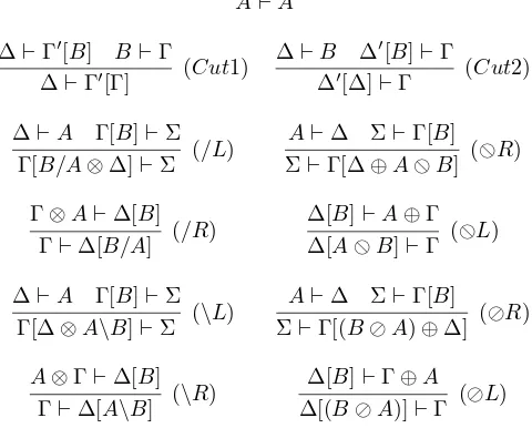
--Figure 1 summarizes the Lambek Grishin calculus in the sequent notation which encodes the mathemat-ical principles represented in Figure 2 that we claim characterize Natural Language Structure. In Figure 2, the symbol∼marks that the principles of mix-associativity and mix-commutativity are the symmetric ver-sion of those without it, i.e. they are about\and⊘instead of/and;, respectively. As mentioned above, the axiom stands for the reflexivity (REF) of the⊢. The cut rule encodes the transitivity (TRAN) of the⊢
in the sequent notation by taking into account the fact that the formulasB can occur within structures (Γ′ and∆′) andAandCcan be structures, i.e.∆andΓ, respectively. (See (Bernardi & Moortgat, 2009) for the precise sequent derivation, here we overlook some proof theoretical issues.) The abstractions(/R,\R)
and co-abstractions (⊘L,;L) encode one side of the residuation and dual residuation rule; the other side of residuation is compiled into the function and co-function applications, (/L,\L)and (⊘R,;R). The reader is referred to (Areces & Bernardi, 2004) for a detailed explanation of the relation between the encoding of the mathematical principles into the sequent system.
4
Case study: Quantifier Phrases
A⊢A
∆⊢Γ′[B] B⊢Γ
∆⊢Γ′[Γ] (Cut1)
∆⊢B ∆′[B]⊢Γ
∆′[∆]⊢Γ (Cut2)
∆⊢A Γ[B]⊢Σ Γ[B/A⊗∆]⊢Σ (/L)
A⊢∆ Σ⊢Γ[B] Σ⊢Γ[∆⊕A;B] (;R)
Γ⊗A⊢∆[B] Γ⊢∆[B/A] (/R)
∆[B]⊢A⊕Γ ∆[A;B]⊢Γ (
;L)
∆⊢A Γ[B]⊢Σ Γ[∆⊗A\B]⊢Σ (\L)
A⊢∆ Σ⊢Γ[B] Σ⊢Γ[(B⊘A)⊕∆] (⊘R)
A⊗Γ⊢∆[B] Γ⊢∆[A\B] (\R)
∆[B]⊢Γ⊕A
∆[(B⊘A)]⊢Γ (⊘L)
Figure 1: LG: Sequent Calculus
(REF) A⊢A
(TRAN) if A⊢Band B⊢C,then A⊢C
(RES)C⊢A\B iff A⊗C⊢B iff A⊢B/C
(DRES)(B⊘A)⊢C iff B⊢C⊕A iff C;B⊢A
(⊗MA) (B ⊘ C)⊗A⊢B ⊘ (C⊗A) (⊕MA) (A⊕C)/B⊢A⊕(C/B)
(⊗MC) A⊗(B ⊘ C)⊢B ⊘ (A⊗C) (⊕MC) (C⊕A)/B⊢(C/B)⊕A
(⊗MA∼) A⊗(C⊘B)⊢(A⊗C)⊘B (⊕MA∼) B\(C⊕A)⊢(B\C)⊕A
(⊗MC∼) (C⊘B)⊗A⊢(C⊗A)⊘B (⊕MC∼) B\(A⊕C⊢A⊕(B\C)
occurring in the complement sentence in (2) of (53). Again, the two interpretations differ in the scope relation (>) betweenthinkandevery man, while the syntactic structure is shared.
Natural language offers also cases of bounded scope: structures that delimit the scope of the operators that cannot express their action outsides those boundaries, as illustrated by the scope possibility in (3a) that is not suitable for (3) Finally, it has been shown (Szabolcsi, 1997) that quantifiers differ in their scope behaviour as exemplified in (4).
(53)
(1) [Someone[knows everyone]vp]s
a. There exists someone that everyone knows [someone>everyone]
b. For everyone there is someone that he knows [everyone>someone]
(2) [Loridp[thinks[every man is immortal]s]vp]s
a. Lori thinks that being immortal is characteristic of men. [thinks>every man]
b. Lori thinks of every actual man that he is immortal. [every man>think]
(3) Two politicians spy on [someone from every city]
a. *every city>two politicians>someone
(4) Lori [didn’t [read QP]]
a. Lori didn’t read a book [Not>A], [A>Not]
b. Lori didn’t read every book [Not>Every], [*Every>Not]
As clearly explained in (Szabolcsi, 2008), this mismatch between syntax and semantics exhibited by quantifiers might call for a distinction between syntactic domain and semantic scope, where the former has been defined in terms of c-command, maximal projection, feature inheritance, or other similar notions, while the latter is the part of the structure on which the operator performs its action, its scope. The hypoth-esis below, originally proposed in (Reinhart, 1979), has found many supporters among linguists. Basically, the claim is that syntactic structure “determines” semantic scope.
(54) “The scope of a linguistic operator coincides with its domain in some syntactic representation that the operator is part of.”
The reader interested in an up-to-date overview of the QP problem and to the several solutions proposed in the literature is referred to (Szabolcsi, 2008) and (Ruys & Winter, 2009). Here we mention the two well known solutions of the quantifiers puzzle proposed in (May, 1977) and in (Hendriks, 1993), since they will help highlighting some important aspects of our proposal.
May’s approach produces semantic constituent structures in abstract level. May proposes that syntax does not end with producing the surface string. Instead, a movement rule, called “Quantifier raising” (QR) continues to operate at an abstract level, called the “Logical Form” (LF), and attach each phrase containing a quantifier to its domain by splitting the node S of the surface structure into two nodes. The rule leaves a virtual tracetcoindexed with the moved QP. Its earliest formulation operates as shown below.
(55)
S
. . . QP . . .
⇒ S
QPi S
QR may derive from one given surface structure several different LFs with different scope relations. The structures at the LF level are then interpreted obtaining the meaning representations.
In the solution we propose the syntactic tree is not re-written into a semantic tree, rather the QP category splits into two parts: the syntactic-component,dp, that actually stays in the syntactic structure – where in May’s LF there is a virtual tracet– and it’s only the scope-component that moves out and reaches the top S-node of the sentence where the QP performs its action.
Hendriks dissociates scope from pure syntax in that it allows one to maintain whatever constituent structure seems independently motivated and still delivers all imaginable scope relations: all the possible scope relations can be obtained by means of three type-change rules: “Argument Raising”, “Value Raising”, and “Argument Lowering”. As we have seen in (26), the last two are already theorems of NL , whereas “Argument Raising” is not. A relevant instance of it is instead a theorem in LG : the argument of a transitive verb can be raised to the higher order category of quantifiers, as we show in (61). See (Bastenhof, 2007) for further details.
As emphasized in (Szabolcsi, 2008), an important task for researchers working on the syntax-semantic interface is “to determine whether the Reinhart’s hypothesis is correct and if yes, exactly what kind of syntactic representation and notion of domain bears it out”. In the logic perspective, the question reads as saying which are the logical operators that capture this connection between the two components of quantifiers, while allowing to scope over the top part of a tree and still remain in the original position as a dp. NL does not provide us with the required tools. It is the minimum logic to model local dependency and the assembly of direct scope constructors, but it is too weak to account for long-distance dependency, cross-dependencies and inverse scope effects. Hence, the need of a more expressive logic that goes behind these limitations. Below we show how LG properly captures the QP unbounded scope behaviour exhibited in the examples (1) and (2) above. We believe that the different scope distribution of QPs ((4) in (53)) can be accounted for by adding unary modalities to LG following (Bernardi, 2002; Bernardi & Szabolcsi, 2008). Following (Barker & Shan, 2006), we conjecture that the cases of bounded scope ((3) in (53)) are properly handled by delimited continuations which belong to the framework we have presented here. For reason of space we cannot go into the details of continuation semantics; in Section 5 we sketch its connection with LG and refer the reader to (Bernardi & Moortgat, 2009; Bastenhof, 2009a).
The “parsing as deduction” view on QP Let us use an example to guide our analysis of QPs. Take the
sentenceAlex thinks everyone left. The proof of its grammaticality corresponds to the following sequent where we leave the QP category undefined.
(56) dp
|{z}
alex
⊗((dp\s)/s
| {z }
[thinks
⊗( QP
|{z}
[everyone
⊗dp\s
| {z }
left]]
))⊢s
Our task, now, is to understand which is the category to be assigned to QP. Recall the conclusion we reached while observing the quantifiers’ semantic constituent tree ((38) in Section 2.4): a quantifier consists of a syntactic and a semantic component (thedpand a function fromstos), such that (a) thedpshould stay in the embedded position where it works as an argument of a verb, and (b) the scope component should be free to travel through the tree so to reach its top level, without modifying the constituent structure. In other words, we start from a structure containing a QP, that isΓ[QP], which is proved to be of categorys, if the simpler structureΓ[dp]is of categorysand the semantic components of the QP reaches the top of the structure. In the following, we will explain what it means for the QP to “reach the top” of the structure and how it does it. This behaviour is captured by the co-abstraction rule which happens within an⊗-structure
Γcontaining the QP that, for the moment, we represent asB;dp– whereBis the category to be assigned to the QP semantic component and which still needs to be specified.
(57)
Γ[dp]⊢B⊕s
Γ[B;dp]⊢s (;L)
(58) s⊢B⊕s
We want to know what could be the proper category to replaceB. By dual residuation (DRES in Figure 2), we obtain that the semantic component of a QP is the co-functor category(s⊘s). We repeat in (59) the if-part of DRES we use below:
(59) (DRES) C⊢B⊕A iff C⊘A⊢B
(60) s⊢B⊕s iff (s⊘s)⊢B
Hence, the whole category of a quantifier should be(s⊘s);dp, where the value-sand argument-sare the first and second one, respectively, viz.(sarg⊘sval);dp.9 Before going to look at some linguistic
examples, it’s worth underline the following two facts.
First of all, as the reader can check by herself,(s⊘s);dp⊢s/(dp\s): every expression that belongs to the non-local scope category, belongs to the local category too; whereass/(dp\s) 6⊢ (s⊘s);dp. Moreover, whereas the “Argument Raising” is not a theorem of LG (see (26) in Section 2), the argument of a transitive verb can be raised to the QP category as shown below. In (Bastenhof, 2007), this theorem is used to handle the interaction of QPs with intentional verbs.
(61)
.. ..
dp⊗((dp\s)/dp⊗dp)⊢(s⊘s)⊕s dp⊗((dp\s)/dp⊗((s⊘s);dp))⊢s (;L) dp⊗((dp\s)/dp⊗(((s⊘s);dp)))⊢s
(dp\s)/dp⊗((s⊘s);dp)⊢dp\s (\R)
(dp\s)/dp⊢(dp\s)/(((s⊘s);dp)) (/R)
Looking at the categories obtained in terms of the two merging relations, saying thatQP ∈(s⊘s);dp means that there are two partsyandxsuch thatMergec
(y, QP, x),y6∈(s⊘s)andx∈dp. In other words, we obtain the syntactic componentxby extracting the semantic componentzfrom the QP. The syntactic componentx ∈ dpwill stay in the⊗-structure where it can merge with other expressions, whereas the semantic component will go to the⊕-structure.
Let’s check how this category behaves by looking at direct and inverse scope caused by a QP in sub-ject (62) and obsub-ject position (63), respectively. As the reader can check by herself, the application of the
(\L)(and(/L)) in (62) (resp. (63)) builds a derivation that does not end with axiom links –hence it fails to prove that the sequent holds. The only other possible first step is the application of(;L).
(62)
dp1⊢dp2
s3⊢s1 s2⊢s4
s3⊢(s1⊘s2)⊕s4 (⊘R)
dp1⊗(dp2\s3)⊢(s1⊘s2)⊕s4 (\L)
((s1⊘s2);dp1)
| {z }
everyone
⊗(dp2\s3)
| {z }
left
⊢s4 (;L)
(63)
s1⊢s2 s3⊢s4
s1⊢(s2⊘s3)⊕s4 (⊘R)
.. ..
dp1⊗((dp2\s1)/dp3⊗dp4))⊢(s2⊘s3)⊕s4
dp1
|{z}
[Alex
⊗((dp2\s1)/dp3
| {z }
[knows
⊗((s2⊘s3);dp4)
| {z }
everyone]]
)⊢s4 (;L)
With the first inference step, the co-abstraction (;L), the scope-component of the QP (sarg⊘sval) is sent to the succedent of the⊢leaving on the antecedent a standard⊗-structure, the syntactic constituent structure of the sentence, containing adp in the place of the QP. By function application steps, this structure is reduced to the categorys carried by its head, the verb, (s3 in (62) ands1 in (63)) – in (64), we will
reachessarg (s3 ⊢ s1in (62), ands1 ⊢ s2 in (63)) andsvalreachessgoal (s2 ⊢ s4in (62) ands3 ⊢ s4
in (63)).
As introduced in (46) of Section 3, we use a tree for the left side of the sequent and a mirror upside down tree for its right side; we obtain the division of labor below, where the upside down tree represents the semantic constituent structure (which plays the role of May’s LF) and the usual tree the syntactic structure. The first inference step (;L) in the two sequents corresponds to the schematic trees in (64) below.
(64)
QP
•
s
goalIf
•
⊗
⊕
dp
⊗
s
arg!
s
vals
goalTo ease the comparison with the sequents above, we can represent the tree on the right in (64) as following:
(65)
dp
⊗
⊕
s
goals
vhd!
s
args
arg!
s
valwhere thesvhdstands for thessub-formula of the category representing the head of the predicate argument
structure, viz. thesvalue of the main verb.
The tree, containing thedpcomponent of QP, is reduced tosvhdwhich reaches (⊢) thesargof the QP’s
scope component and thesvalreaches thesgoal.
It is interesting to compare (65) with the QR schema (55); we repeat it in (66) with the annotation of the S-nodes to help grasping the similarity between the two solutions: LG captures the mathematical principles behind QR.
(66)
Sgoal
. . . QP . . .
⇒ Sgoal
QPi Svhd
. . . ti. . .
The “parsing as deduction” view on Scope Ambiguity The simplest case with scope ambiguity is the one with QPs both in subject and object positions [Someone [knows everyone]]. The sequent to prove is:
(67) ((s1⊘s2);dp1)
| {z }
[someone
⊗((dp2\s3)/dp3
| {z }
[knows
⊗((s4⊘s5);dp4)
| {z }
everyone]]
)⊢s6
There are three main functional connectives (two ;and one/) in the antecedent of the sequent that could be activated, hence three inference rules could be applied. As the reader can check by herself, the application of the(/L)rule builds a derivation that does not end with axiom links –hence it fails to prove that the sequent holds. The other two possibilities are(;L)applied to the;of the subject or of