Competitive Moment Matching
of a New-Keynesian and an Old-Keynesian Model:
Extended Version, First Draft
Reiner Frankea,∗
May 2012
aUniversity of Kiel, Germany
Abstract
The paper considers two rival models referring to the new macroeconomic consensus: a standard three-equations model of the New-Keynesian variety and dynamic adjustments of a business and an inflation climate in an ‘Old-Keynesian’ tradition. Over the two subperiods of the Great Inflation and Great Moderation, both of them are estimated by the method of simulated moments. An innovative feature is here that it does not only include the autocovariances up to eight lags of quarterly output, inflation and the interest rate, but optionally also a measure of the raggedness of the three variables. In short, the performance of the Old-Keynesian model is very satisfactory and similar to, unless better than, the New-Keynesian model. In particular, the Old-Keynesian model is better suited to match the new moments without deteriorating the original second moments too much.
JEL classification: C52; E32; E37.
Keywords: Sentiment dynamics; new macroeconomic consensus; method of simulated moments; Great Inflation, Great Moderation.
∗ Corresponding author.
1. Introduction
The paper brings together two strands of economic research on small-scale modelling in the context of the so-called new macroeconomic consensus. First, there is the New-Keynesian approach with its extensive estimation literature. While Bayesian likelihood methods have become dominant here in the past decade, a smaller number of studies has alternatively used moment matching procedures. They seek for parameter values such that a set of model-generated summary statistics, or ‘moments’, comes as close as possible to their empirical counterparts. The goodness-of-fit of a model, or a trade-off between the merits and demerits in matching specific moments, can thus also be assessed in finer detail than by just referring to the optimization of a single and relatively abstract objective function.
In particular, this method has recently been applied to a hybrid three-equations model with forward- and backward-looking elements, which focusses on the quarterly output gap, the inflation gap and the interest gap (i.e., the deviations of these variables from a constant or possibly time-varying trend). Within mainstream macroeconomics, the model represents a sort of common-sense middle ground that preserves the insights of standard rational expectations with some sort of sluggish behaviour, while allowing for better empirical fit by dealing directly with a well-known empirical deficiency of the purely forward-looking models. As a result, this class of models has been widely used in applied monetary policy analysis, with the policy implications depending importantly on the values of the coefficients on the expected and lagged variables, respectively.
When estimating the New-Keynesian model, the moments to be matched were the auto- and cross-covariances of the three variables with lags up to eight quarters. Admit-ting sufficiently backward-looking behaviour (in some contrast to the ordinary likelihood literature), the performance of these estimations on US data for the two sub-periods of the so-called Great Inflation and Great Moderation was so good that they were said to constitute a challenging yardstick for any macroeconomic model of a similar complexity (Franke, 2011a; Franke et al., 2011).
The second strand of research that we address are macroeconomic theories that refuse the paradigm of the optimizing representative agents and their rational expectations. To face the task of providing strong alternatives, two new types of models have been advanced within the three-variables framework that put special emphasis on translating the idea of the famous ‘animal spirits’ into a formal canonical framework. They can thus be briefly characterized as models of sentiment dynamics (Franke, 2008 and 2011a; De Grauwe, 2010). Their cycle-generating properties have been demonstrated by numerical simulations with suitably calibrated parameters, but so far these models have not yet been subjected to econometric procedures.
the individual firms switch between an optimistic and a pessimistic investment attitude. In addition, entering the Phillips curve is an inflation climate the adjustments of which are influenced by a parameter that represents the general credibility of the central bank. For a better contrast, this model is called an Old-Keynesian model. Because of its intrin-sic nonlinearities, the second moments for the estimation can no longer be analytically computed as in the linear New-Keynesian case but have to be simulated over a long time horizon (which introduces the problem of sample variability). The obvious question is, of course, whether the general match of the Old-Keynesian model can compete with the New-Keynesian model (NKM).
Three different versions of the Old-Keynesian model are studied. The first one is deterministic and the exact discrete-time analogue of Franke (2011a), except that it slightly extends the Taylor rule in order to have the same specification with interest rate smoothing as in NKM. The persistent cyclical behaviour in this model is mainly brought about by a sufficiently strong herding mechanism; it renders the long-run equilibrium unstable, while the nonlinearities prevent the dynamics from exploding. The goodness-of-fit that can here be achieved deserves already some respect, although it will clearly fall behind the stochastic NKM.
Versions two and three of our model are stochastic, which, incidentally, will deempha-size the role of herding in the estimations. They introduce the analogous quarterly ran-dom shocks from NKM, i.e. demand shocks, supply shocks and monetary policy shocks, all of them being serially uncorrelated. In the second version they only take direct effect in an output equation, the Phillips curve and the Taylor rule, respectively. Being inspired by NKM where in the reduced-form solution each shock acts on each of the three vari-ables, our third version additionally allows the demand shock to act on the adjustments of the inflation climate and the cost push shock to act on the adjustments of the firms’ investment attitude.
When estimating the models with the second moments mentioned above one will note that the general pattern of the simulated time series exhibits a similar level of noise. This is in contrast to the empirical series where the quarterly inflation rates are much noisier than the other two variables. As an innovative feature we specify a measure of raggedness of the time series and add these statistics to the other moments. By and large it turns out that the Old-Keynesian model is better suited to match the new moments without deteriorating the original second moments too much. A short and succinct characteriza-tion of the overall matching quality will then be that the second version is fairly similar to that of NKM, whereas the third version is markedly superior. The paper thus shows that, in the framework indicated, there is indeed an alternative ‘Old-Keynesian’ model that can well bear comparison with the workhorse model of orthodox macroeconomics.
in Sections 4 and 5, where Section 4 deals the period of the Great Inflation and Section 5 with the Great Moderation. Section 4 is actually the main part of the paper as it also contains the discussion of many specification details when they are first applied. Section 6 concludes. Several more technical issues are relegated to a number of appendices.
2. The estimation approach
2.1. The minimization problem
The approach to estimate our New- and Old-Keynesian models is concerned with their dynamic properties in general. They are quantitatively described by a number of sum-mary statistics, also called ‘moments’, and the estimation seeks to identify numerical parameter values such that the model-generated moments come as close as possible to their empirical counterparts. In linear models such as the log-linearized New-Keynesian rational expectations models, all or a larger set of the moments can be computed ana-lytically. If this is not possible, which because of its nonlinearity will be the case for the Old-Keynesian model, the moments can still be computed from numerical simulations of the model. Hence, briefly, we are using the method of moments (MM) or the method of simulated moments (MSM), respectively.
The crucial point is, of course, the choice of the moments, which by some critics is branded as arbitrary. Here the approximate nature of modelling should be taken into account. Since any structural model focusses on a specific purpose, it is only natural that it would be able to match, at best,someof the ‘stylized facts’ of an actual economy. MM and MSM, then, require the researcher to definitely make up his or her mind about the dimensions along which the model should be most realistic. Correspondingly, one can look at the single moments and find out which of them are more adequately matched than others. This will also provide more detailed diagnostics about the particular merits and demerits of a model than an objective function that summarizes many (and perhaps infinitely many) features in a single value. In our view, it is the explicit choice of the moments and, in practice, their easy interpretation that are strong arguments just in favour of the moment matching approach.1
Generally, there arenm moments that are collected in a column vectorm∈IRnm. The
moments that are obtained from an empirical sample of T observations are designated mempT . The model-generated moments depend on the numerical values of a vectorθofnθ
structural parameters, which are confined to a (rectangular) set Θ⊂IRnθ. If analytical
expressions for these moments are available (which are the asymptotic moments), we could unambiguously writem=m(θ). If the moments have to be simulated, the
tion size should be made explicit, i.e., the effective number of periods S over which the model is simulated. As an approximation to the infinite simulation size that would be needed for the asymptotic moments, the final estimations of our discrete-time, quarterly models will be based on S= 10,000 quarters.2
The long time horizon reduces, but does not completely eliminate, the sample variabil-ity from different random number sequences that are underlying the simulations when the models are stochastic. These sequences may be identified by a natural numberc∈IN, which corresponds to their random seed. In sum, a model-generated vector of moments is thus determined asm=m(θ;c, S).
The distance between the vectors of the theoretical and empirical moments is measured by a quadratic functionJ that is characterized by an (nm×nm) weighting matrixW. The
value of this loss function is to be minimized, where it goes without saying that across different parameters θ only simulations with the same random seed are comparable.3 Accordingly, the model is estimated by the following set of parameters:
b
The problem of how to treat the variability arising from different random seeds c is addressed below.4
Minimization of (1) is not a straightforward matter. Given the relatively high number of parameters in our applications, there is for functions of type (1), just as it is the case for likelihood functions, a great danger of a larger number of local extrema, possibly also located at a farther distance from each other. Our search therefore proceeds in two steps. First, in order to reduce the risk of being trapped in a wrong region of the parameter space, we use simulated annealing as a globally effective procedure.5
2 “Effective” simulation size means that, starting from the steady state position, the models are simulated over 200+Squarters and the first 200 quarters are discarded to rule out any transient effects (which proves to be more than sufficient).
3 For our random variables, which are of the form ε
t ∼ N(0, σ2), this means that in period
t always the same random number ˜εt is drawn from the standard normal N(0,1) and then, depending on the specific value ofσunder examination,εtis set equal toεt=σε˜t.
4 If in the course of the minimization search procedure for (1) some parameter leaves an ad-missible interval, it is temporarily reset to the boundary value, the loss J of the thus resulting moments is computed, and then a sufficiently strong penalty is added toJ that proportionately increases with the extent of the original violation. In this way also corner solutions to (1) can be safely identified.
Since, with different initial conditions and different random sequences for the stochas-tic search, the algorithm does not always settle down in the same region, it is necessary to carry out several minimization runs and identify from them a parameter region with the lowest losses. A situation typically encountered is that two or four out of ten runs fail to find sufficiently low values of the loss function, while the remaining trials yield fairly close values in the same region.6
In a second stage, we choose the optimal parameter vector from the stage of simu-lated annealing and take it as a starting vector for another minimization procedure, the Nelder-Mead simplex search algorithm (see Press et al., 1986, pp. 289–293).7 Even when
repeatedly restarting it upon convergence until no more noteworthy improvement in the minimization occurs, this algorithm is faster than simulated annealing (it takes a few minutes). Combining the two search strategies, we can be rather confident that for all practical purposes the global minimum of (1) has indeed been found.
Turning to the weighting matrix W that sets up the loss function in (1), an obvious since asymptotically optimal choice would be the inverse of an estimated moment covari-ance matrix Σbm (Newey and McFadden, 1994, pp. 2164f). Unfortunately, the moments
underlying our estimations will not be independent of each other, so that such a matrix would be nearly singular and its inverse could not be relied on. The usual option, then, is to employ a diagonal weighting matrix the entries of which are given by the reciprocals of the variances of the single moments.
There are several methods to estimate these variances from the empirical data. Here we employ a bootstrap procedure. It is in detail somewhat different from an ordinary block bootstrap but seems more appropriate to us for the present problem (the details are described in Appendix A1). This being understood, we have
Wii = 1/ Var(d mempT,i ), i= 1, . . . nm (2)
(and of course Wij = 0 if i6= j). Clearly, the less precisely a moment is estimated
from the data, that is, the higher is its variance, the lower is the weight attached to it in the loss function. Since the width of the confidence intervals around the empirical momentsmempT,i is proportional to the square root of these variances, it may be stated that the model-generated moments obtained from the estimated parameters lie “as much as possible inside these confidence intervals” (Christiano et al., 2005, p. 17). Nevertheless, a formulation of this kind, which with almost the same words can also be found in several other applications, should not be interpreted too narrowly. In particular, a minimum of
subsequently Boltzmann’s formula exp(−M/To) = 0.50 is solved forTo.
6 A shorter simulation horizon ofS = 2,000 proves to be sufficient for these global investigations. The reduction is helpful here since on average one such run takes about 25 minutes on a standard personal computer.
the loss function in (1) need not simultaneously imply a minimal number of moments outside the confidence intervals.8
As useful feature of the approach of moment matching is that it does not only provide a measure of the model’s overall goodness-of-fit, it also allows us to locate potential shortcomings in single moments. A convenient since directly available measure to evaluate how serious the deviations of a model-generated moment from the empirical moment may be can be obtained by relating them to the standard errors of the latter. With respect to a moment i, this is the t-statistic
ti = [mi(θ;c, S) − mempT,i ]/ q
d
Var(mempT,i ) , i= 1, . . . nm (3)
(reference ofti tocandSis omitted as it will be understood from the context). Although
statistically not exactly justified, we would be satisfied with the matching of a moment if itst-statistic will be less than two in absolute value; otherwise we would have to admit that the model has a certain weakness in this respect. It may also be noted in passing that, with the diagonal weighting matrix from (2), estimation means nothing else than minimizing the sum of the squared t-statistics, which is a fairly intuitive criterion.
After thus establishing the econometric framework, we have to turn to the specific moments on which we want to base our estimations. In the course of discussing the results, we will demand more from the models and correspondingly extend the set of these moments. For the time being, we make the matching criterion explicit from which we start out. It is meant to characterize the fundamental dynamic relationships between the observable variables of the model. For this purpose the second moments are well suited, that is, the nine profiles of the unconditional contemporaneous and lagged auto-and cross-covariances of (the gaps of) output (y), inflation (π) and the interest rate (i).9
It may be emphasized that we fix these moments in advance and that their number will not be too small, either.10 In detail, we are concerned with the nine profiles of
Cov(pt, qt−h) forp, q=i, y, π andh= 0,1, . . . up to some maximal lagH (the hat over
iorπ for the New-Keynesian model below may be omitted here). Given that the length of the business cycles in the US economy varies between (roughly) five and ten years, the estimations should not be based on too long a lag horizon. A reasonable compromise is a length of two years, so that we will work with H = 8 quarters. In this way we have a total of 78 moments to match: 9 profiles with (1+8) lags, minus 3 moments to avoid double counting the zero lags in the cross relationships. To distinguish it from the
8 An example for this can be found in Franke et al. (2011, p. 11, Table 1).
9 The second moments provide similar information to the impulse-response functions of the three types of shocks in the models, in which (or just one of them) many New-Keynesian studies take a greater interest.
extended versions below, we denote this loss function by J(78). For a definite reference, we repeat
J(78): loss function constituted by the 78 moments Cov(pt, qt−h)
and the corresponding weightsWii from (2),
forp, q=i, y, π and h= 0,1, . . . ,8
(4)
2.2. Confidence intervals and J test
Under standard regularity conditions, the parameter estimatesθbfrom (1) are consistent and asymptotically follow a normal distribution around the (pseudo-) true parameter vector. There is moreover an explicit formula for estimates of the corresponding covari-ance matrix, from which the standard errors of θb are obtained as the square roots of its diagonal elements (Lee and Ingram, 1991, p. 202). In the present case, however, this approach faces two problems. First, it may turn out that locally the loss function J may react only very weakly to the changes in some of the parameters. Hence these stan-dard errors become extremely large and, beyond this qualitative message, are not very informative. The second point is that one of the regularity conditions will be violated if the minimizing parameter vector is a corner solution of (1) or close to an upper- or lower-bound of some parameter; trivially, for some componentsithe distributions of the estimated parameters cannot be symmetrically centred around the point estimates θbi
then.
These problems can be avoided by having recourse to a bootstrap procedure. Besides, it is also expedient for coping with the small sample problem. In this respect it is only natural to employ the bootstrap that already served to obtain the variances of the em-pirical moments in the weighting matrix W above. From there we have a large set of artificial moments on which, rather than on the single empirical moment vectormempT , a model can be re-estimated just as many times as we want. In this way we get a frequency distribution for each of the parameters and can easily compute the confidence intervals from them (see below).
(DGP). Hence the distribution of the lossesJeincurred from them would lend us a test criterion for a possible rejection of the model, which we would have to do if the previously estimated value J[θb(c, S);mempT , c, S] exceeds the 95% quantile of theseJe.
Although this concept is straightforward, the precise specification of the re-estimation problem requires a little care. Denoting the distribution of the bootstrapped moment vectors by {meT} and omitting the reference to c and S for a moment, it has to be
taken into account that, except for special circumstances, there is no set of parametersθ ensuringE[m(θ)−meT] = 0 (as there are more moments than parameters in the model).
This fact becomes important for the first-order validity of the bootstrapped J test, for which a null hypothesis must be imposed.11 To this end we first observe thatE(me
T) =
mempT should prevail. Furthermore, different (hypothetical) realizations of the real-world DGP would give rise to a distribution of the estimated parameters bθand corresponding moment vectorsm(θb), while the parameters eθthat are re-estimated on the bootstrapped moments give rise to a distribution m(θe). These two moment distributions should have the same mean values, too; that is, E[m(θe)] =E[m(θb)] is supposed to hold true. Taken together, we get the equation E{[m(θe)−meT] − [m(θb)−mempT ]}= 0. Writing it in this
form makes it clear that the moment conditions for the bootstrap version of the J test are to be demeaned by the second term in square brackets.
The corresponding MSM re-estimations take two types of variability into account. First, we allow for the variability in the generation of the data. To this end we apply the procedure in Appendix A1 that we already referred to above, which gives us a collection {mb
T}Bb=1 of B moment vectors bootstrapped from the empirical time series of length
T. Second, we allow for the sample variability in the model simulations by carrying out each estimation with a different seed c. Thus, practically, each bootstrap sample b has associated with it a random seed c=c(b).
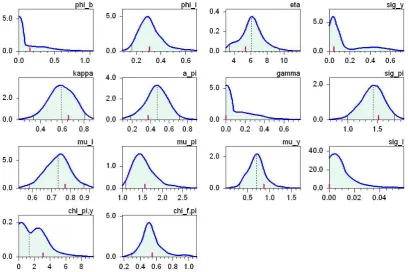
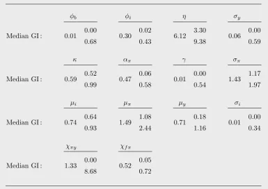
In addition, suppose that we have a large number of original estimations (1) on the empirical moment vectormempT . Then, let us settle down on the random seed ¯cthat yields their median loss. That is,θb(¯c, S) is our benchmark point estimate of the model. On this basis, the collection of the parameter re-estimates θbb is obtained as follows:
b
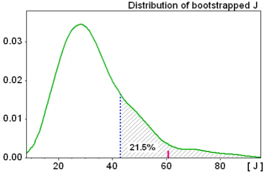
For the bootstrapped J test it remains to consider the distribution of the values Jb g =
Jg(θbb;b). At the conventional significance level, the model with estimate θb(¯c, S) would
have to be rejected as being inconsistent with the data if the corresponding loss Jb= J[θb(¯c, S);mempT ,¯c, S)] from (1) exceeds the 95% quantile of the distribution {Jb
g},
wise the model would have passed the test. In this way we can also readily construct a p-value of the model. It is given by the value ofp that equates the (1−p)-quantile of the distribution {Jb
g} to Jb, which says that if Jbwere employed as a benchmark for model
rejection, then p is the error rate of falsely rejecting the null hypothesis that the model is the true DGP. Hence, in short, the higher thisp-value the better the fit. Certainly, it may not be forgotten that, besides sample variability, this evaluation is conditional on the specific choice of the moments that the model is required to match.12
Regarding the confidence intervals that, from the re-estimations, can be built for the i-th component of the originally estimated parameter vector bθ(¯c, S), two versions can be set up: the standard percentile interval and Hall’s percentile confidence interval. Hall’s method has the advantage that it is asymptotically correct, but it may violate the admissible range of a parameter. Therefore we use Hall’s interval if no such violation occurs and the standard interval otherwise. The details are spelled out in Appendix A2, equations (A1) and (A2).
Having available a reliable estimate θb(¯c, S), the minimizations in (5) can safely do without further global explorations. That is, we can directly use the simplex algorithm for them and let it start from a simplex around θb(¯c, S). Nevertheless, although a single minimization with several re-initializations does not take very long, the computational effort for, say, a battery of 1000 re-estimation accumulates considerably. For this reason we will only make use of this method for our ‘showcase’ estimations. For the other versions we content ourselves with the point estimations based on the same random seed ¯cas the median loss of the best model version. They will not be perfect but good enough to indicate the basic tendencies to us.
3. The two Keynesian approaches
3.1. The New-Keynesian model
The elementary New-Keynesian models are constituted by three equations determining output, inflation and the rate of interest. It should be made clear from the beginning that we are concerned with these variables in gap form, that is, with their deviations from some trend values.13 The exact specification of the latter depends on the partic-ular microfoundation from which the equations are derived. In the simpler versions at a textbook level, the ‘trend’ is just a fixed steady state value, which for the inflation
12An application of this bootstrap approach to another New-Keynesian model is F`eve et al. (2009), although they only estimate a subset of the parameters. Their moments are given by the impulse-response functions to a monetary policy shock, so that they can be analytically computed and thep-value is not plagued with the sample variability fromc=c(b).
rate will furthermore be equal to zero. More generally, the trend may be given by some moving frictionless output equilibrium or by time-varying target rates of inflation and interest set by the central bank. To allow for a wider range of theoretical interpreta-tions, we will treat the trend as a purely exogenous issue.14 It can therefore remain in the background, so that, with respect to period t, the formulation of the model directly refers to the output gap yt, the inflation gapbπt, and the interest rate gapbit.15 On this
basis the New-Keynesian model, labelled ‘NK’, that we are going to estimate reads:
yt = φyEtyt+1 + (1−φy)yt−1 − τ(bit−Etbπt+1) + vy,t (0≤φy ≤1) b
πt = φπβ Etπbt+1 + (1−φπ)βbπt−1 + κ yt + vπ,t (0≤φπ ≤1) bit = µrbit−1 + (1−µr) (µπbπt + µyyt) + εr,t
vπ,t = ρπvπ,t−1 + επ,t
vy,t = ρyvy,t−1 + εy,t
(NK)
As already mentioned, the underlying time unit is one quarter. All of the parameters are supposed to be nonnegative, but regarding the order of magnitude of some of them it should be pointed out that the rates of inflation and interest will be annualized. Clearly, (NK) is a hybrid model with forward-looking as well as backward-looking elements in the dynamic IS relationship (the first equation) and the Phillips curve (the second equation, where β is the usual discount factor). As it is standard in this framework, the third equation is a Taylor rule with interest rate smoothing and contemporaneous reactions to inflation and output. It goes without saying that the smoothing coefficientµris contained
in the unit interval.
The same property for φπ and φy in the first two equations of (NK) is less obvious,
which is the reason why it is explicitly scheduled in the equation block. As a matter of fact, the common specifications of the IS equation are based on a habit persistence parameter χ between 0 and 1 that would give rise to a composite coefficientφy = 1/(1+χ)≥1/2.
Concerning the Phillips curve, the two main proposals to establish a positive coefficient on lagged inflationbπt−1 are an introduction of rule-of-thumb price setters (following Gal´ı
and Gertler, 1999), or of an indexation rule on the part of the firms that currently are not permitted to re-optimize their price (following Smets and Wouters, 2003, and Christiano et al., 2005). In both cases the resulting coefficientφπ on expected inflation must exceed
one-half (roughly), too.16
14Ireland (2007) and, more ambitiously, Cogley and Sbordone (2008) are two proposals of an en-dogenous determination of the central bank’s moving inflation target. Ireland (p. 1864), however, concludes from his estimations that still “considerable uncertainty remains about the true source of movements in the Federal Reserve’s inflation target”.
15In the verbal discussions we may nevertheless omit mentioning the ‘gap’ and, for instance, simply speak of inflation.
While the standard microfoundations are based on zero inflation and the absence of output growth in the steady state, there is more recent work relaxing these assumptions. The price to be paid for this step towards realism are (much) more complicated rela-tionships.17 System (NK) in its desirable clarity could nevertheless still be viewed as an approximation to the more ambitious generalizations in this field of macroeconomic theory, arguing that a good understanding of its properties should come in handy before engaging in more specialized versions.
The only microfounded approach we know of that admits a dominance of backward-looking behaviour, in the sense thatφπ orφy are also permitted to be less than one-half,
is that of Branch and McGough (2009).18 Their paper sets up an economy in which
rational expectations coexist with boundedly rational expectations. Introducing a set of axioms for consistent heterogenous expectations and their aggregation, the authors derive a purely forward-looking Phillips curve and IS equation where, however, the ex-pectation operator is a weighted average of the two types of exex-pectations. Thus, in the present notation, φπ and φx can be interpreted as the population shares of the firms
and households, respectively, that entertain rational expectations.19 Moreover, the ex-act form in (NK) with just one lagged inflation rate and output gap on the right-hand side is obtained if the group of the non-rational agents is supposed to have static expec-tations, that is, if (perhaps for lack of a better or more reliable idea) they do not expect the value of the variable from their last observation to change until the next quarter.
The foundation proposed by Branch and McGough (2009) appears to be an attractive alternative to motivate a general formulation like (NK); in particular, if estimations would prefer lower values of φπ or φy outside the conventional range. Note that (NK) would
even be well-defined ifφπ orφy were zero and all of the firms or households, respectively,
were purely backward-looking. On the other hand, besides the fact that this economy is still stationary and does not allow for long-run inflation, and besides thinking of less naive than just static expectations, a critical point of the approach is a justification of why the population sharesφπ andφy should remain fixed over time. Extensions of (NK)
taking this issue into account are easily conceivable but beyond the scope of the present
standards of New-Keynesian modelling. Two examples of well-established authors who rather characterize them as an ad hoc amendment are Fuhrer (2006, p. 50) and Rudd and Whelan (2005, pp. 20f), which is the more detailed version of Rudd and Whelan (2007, p. 163, fn 7). 17Contributions with positive trend inflation are Bakshi et al. (2003), Sahuc (2006), Ascari and Ropele (2007), Ireland (2007), and Cogley and Sbordone (2008), among others. Mattesini and Nistic`o (2010) incorporate positive trend growth.
18Fuhrer (2006) is a study of a Phillips curve similar to that in (NK) which likewise does not require, or imply, thatφπ (in the present notation) is positively bounded away from zero. In his discussion of the inflation persistence effects that strongly favours low values ofφπ, however, the author does not care about a rigorous structural interpretation of these situations.
paper.20
Turning to the stochastic pert of the model, each of the three core equations is aug-mented by an exogenous shock process. In the Phillips curve, serial correlation in the random shocks is included as a possible additional source of inflation persistence. This is in contrast to a common estimation practice that from the outset assumes either white noise shocks in a hybrid Phillips curve, or purely forward-looking price setting behaviour in combination with autocorrelated shocks.21 Here we refrain from this prior decision and try to find out whether the data indicate a certain tendency.
For symmetry, the IS equation should be treated in the same way (although this point seems to have been somewhat neglected in the literature). The shocks in the interest rate reaction function, i.e. the Taylor rule, are i.i.d. and, as it is standard in the three-equations framework, persistence is only supposed to be brought about by the lagged rate of interest. The white noise innovationsεz,t, forz=i, π, y, are mutually uncorrelated and
normally distributed with variance s2z. Certainly 0≤ρπ, ρy <1 in the AR(1) processes
in the last two equations of (NK).
Over the relevant range of the numerical parameters, determinacy of (NK) will prove to be no problem.22 Under this condition, there are two uniquely determined matrices Ω,Φ ∈ IR3×3
(Ω being a stable matrix) such that, with respect to x = (i, y, π)′
, v = (vi, vy, vπ)′, ε= (εi, εy, επ)′ and N ∈ IR3×3 the diagonal matrix with entries (0, ρy, ρπ),
the reduced-form solution to (NK) is given by an ordinary ‘backward-looking’ stochastic difference equations system:
xt = Ωxt−1 + Φvt
vt = N vt−1 + εt
(6)
Calculation of the matrices Ω and Φ is a routine matter in New-Keynesian economics, the details of which can therefore be omitted. Equation (6) is here quoted for a better comparison with the structure of our Old-Keynesian model, which is presented next.
20In another paper, Branch and McGough (2010), the population shares are modelled as en-dogenously changing over time according to a measure of evolutionary fitness, which includes a (relatively higher) cost of forming rational expectations. It is, however, another question beyond the scope of the present paper whether this conceptual progress would also yield a significantly better econometric performance.
21In similar models to ours, examples of i.i.d. shocks in a hybrid Phillips curve are Lind´e (2005), Cho and Moreno (2006) or Salemi (2006), while the purely forward-looking models studied by, e.g., Lubik and Schorfheide (2004), Del Negro and Schorfheide (2004), Schorfheide (2005) permit some persistence in the shock process. These references have been chosen from the discussion in Schorfheide (2008; see p. 421, Table 3).
3.2. The Old-Keynesian model
The Old-Keynesian model that we want to put forward as an alternative to the New-Keynesian model (NK) abjures the representative and intertemporally optimizing agents and their rational expectations. The central notion is rather that of an average business sentiment of firms that either have an optimistic or pessimistic attitude towards the fixed capital investment decisions they face. Jointly with the dynamic law that is to govern its changes over time, this sentiment variable is meant to capture some of the meaning of Keynes’ famous ‘animal spirits’ in a highly stylized manner. These issues and the specification details of this and other model elements are discussed in greater depth in Franke (2011a). Here we content ourselves with a short recapitulation of the model. In addition, we introduce a few extensions in order to put it on a similar footing to the New-Keynesian model.
The present model will deviate from Franke (2011a) in three ways: (i) the continuous-time formulation is transformed into discrete continuous-time, where the continuous-time unit is again a quarter; (ii) the Taylor rule is the same as in (NK), which slightly extends the version without interest rate smoothing in Franke (2011a); (iii) this model, which is still deterministic, will be investigated first, but subsequently random shocks will be included as well.
To begin with the model description, it has already been indicated that the central dynamic variable is the business sentiment, or the business climate, in the firm sector. Denoting it by bt, it is predetermined in period t and given by the difference between
the optimistic and pessimistic firms in this period, scaled by their total number. Hence −1 ≤ bt ≤ 1; the extreme values −1 and +1 are attained if all firms are pessimistic
and optimistic, respectively; and bt = 0 if there are as many optimists as pessimists.
The optimistic firms let their capital stock increase at a given and common high rate of growth, the pessimistic firms at a given and common low rate of growth. This yields the aggregate capital growth rate as a linearly increasing function of the business climate variable.
Total output (or the output-capital ratio) is determined by fixed investment (or the aggregate capital growth rate, respectively)viaa multiplier relationship in a temporary IS equilibrium. Specifying the output gapyt as the percentage deviations of this
output-capital ratio from the value that would prevail in a balanced state bt= 0, yt is easily
seen to be directly proportional to bt with a proportionality factor η > 0. Lastly, for
the general case, we add a normally distributed demand shock εy,t to this relationship.
Since the core of the model should contain sufficient mechanisms to generate any desired degree of persistence, we forego the option of serial correlation in this and the other shock processes. Thus, givenbt in periodt, we have
yt = η bt + εy,t (7)
quarter but to a so-called inflation climate πc
t, which is the firms’ general aggregated
assessment of inflation over a longer time horizon.23 This inflation climate is treated as a predetermined variable, too. Complementing it with supply or cost push shocks επ,t,
the Phillips curve thus reads,
πt = πct + κ yt + επ,t (8)
Output and inflation being determined by (7) and (8), the nominal interest rate it is
subsequently obtained from the Taylor rule with interest rate smoothing. Just as the Phillips curve, we write it here in level form. To this end, we now explicitly introduce the central bank’s target rates of inflation and interest, π⋆ and i⋆, which are supposed
to be constant. This gives us
it = µiit−1 + (1−µi) [i⋆ + µπ(πt−π⋆) + µyyt] + εi,t (9)
A little bit sloppily, eqs (7) – (9) can be said to constitute the static part of the model. The second part describes the updating of the two climate variablesbt andπct. To begin
with the simpler rule, the inflation climate is assumed to adjust, instantaneously or with some delay, to a benchmark that is given by a weighted average of current inflation and target inflation,
πtc+1 = πct + απ[γ π⋆+ (1−γ)πt − πct] + χπyεy,t (10)
Certainly, both the adjustment speed απ and the weight γ are contained in the unit
interval, 0≤απ, γ≤1. The higherγ, the stronger the confidence of firms that inflation
will soon return to its target. For this reason, and for a more formal argument given in Franke (2007, p. 22) or Franke (2011a, Section 3), the parameterγ can be interpreted as representing the credibility of the central bank.24
Another influence on the inflation climate in (10) may be exerted by the demand shocks. That is, positive demand shocksεy,t in (7) could also induce the firms to expect
generally higher inflation rates, not necessarily immediately but with some delay.25 As a
23Franke (2007) discusses the ideas underlying this variable at greater length and also compares its ‘microfoundations’ with heterogenous firms to the New-Keynesian way of deriving a Phillips curve.
24Complementarily, (1−γ) can be interpreted as measuring the inflation persistence in the Phillips curve; see Franke (2007), p. 22. Assimilating an idea from de Grauwe’s (2010) bounded rationality version of the New-Keynesian three-equations model, a more ambitious modelling could introduce two types of inflation attitude between which the firms may switch according to some rule. If one attitude is given byπ⋆ and the other by π
t−1, the role of the coefficientγ in (10) would be taken over by a long-run time average of the share of target inflation believers. The charm of this generalization is that such a central bank credibility would be endogenously determined. On the other hand, for the present model we will be interested in ‘what the data say’ on a specific numerical value of our fixedγ.
consequence, the actual rate of inflationπtis now affected by two shocks, directly byεπ,t
in the Phillips curve and indirectly, from the previous periodviathe climate variableπc t,
by χπyεy,t−1. It may also be said that positive values of χπy indicate ‘crossover effects’
of the demand shocks, from output to inflation.
The motivation for this higher flexibility of the model springs from the structure of system (6), which solves the New-Keynesian model. If the present model, when com-pleted, is analogously decomposed into a deterministic part and a linear stochastic part of the form Φeεt for a suitable matrix Φ with some zero rows, the 3e ×3 nonzero core
of Φ would be a diagonal matrix whene χπy= 0, whereas the entries in the matrix Φ in
(6) are all nonzero. It could thus be said that the shock-free version of eq. (10) puts the stochastic structure of the present model at a certain disadvantage in comparison with its New-Keynesian competitor. Admitting χπy >0 is meant to make up for this. In this
respect it may be noted that in the matrix Φ many zero entries would still remain; one the other hand, the nine entries in Φ are not all independent, either. Nonetheless, in the end we will leave it to the estimations whether or not they call for a positive value of χπy.
The adjustments of the business climatebt are conceptually more involved. They are
based on the uniform transition probabilities prob−+
t and prob+
−
t with which, within
the current quarter t, a single pessimistic (optimistic) firm switches to an optimistic (pessimistic) investment attitude. Assuming a sufficiently large number of firms, the probabilistic elements become negligible at the macro level. The changes in the business climate bt are then easily seen to be described described by the following deterministic
adjustment equation,
bt+1 = bt + (1−bt) probt−+ − (1+bt) prob+t− (11)
The probabilities in (11) are functions of a so-called feedback index ft, where higher
values offt increase the probability of switching from pessimism to optimism. Assuming
symmetry and linearity with respect to relative changes, the transition probabilities of the firms are given by
The coefficient αb measures the general responsiveness of the transition probabilities to
the arrival of new information, as it is summarized byft. It may thus be characterized as
a flexibility parameter (Weidlich and Haag, 1983, p. 41). Note that even in the absence of active feedback forces in the indexft, or when the different feedback variables behind
ft neutralize each other such that ft = 0, the individual firms will still change their
attitude with a positive probability. These reversals, which can occur in either direction,
are ascribed to idiosyncratic circumstances, and their probability per quarter is given by prob−+
t = prob+
−
t = αb > 0.
In the determination of the feedback indexft, two components are distinguished. The
first grasps the idea of herding, saying that the probability of switching from pessimistic to optimistic increases as the population share of the firms that are already optimistic increases. The second component can be conceived of as a counterpart of the central stabilizing effect in the so-called new macroeconomic consensus, which is the real interest rate transmission mechanism of monetary policy. It is correspondingly assumed that optimism in the investment decisions tends to decline as the real interest rate increases. Combining the components in a linear way, we have ft = φbbt −φi(it−πt−ρ⋆) so far,
where φb, φi ≥ 0 andρ⋆ is the long-run equilibrium real rate of interest (from which i⋆
in the Taylor rule derives asi⋆ =ρ⋆+π⋆).
In addition, we want to allow for a possible influence of the random shocksεπ,t in the
Phillips curve. Viewing them as cost pushes, positive shocks somewhat darken the pros-pects of the firms’ future profitability and so tend to weaken their optimism. Introducing another coefficient χf π ≥0 and augmenting the equation above by this effect, which in
the end is a crossover random effect from inflation to output, the following functional expression for the feedback indexft is postulated:
ft = φbbt − φi(it−πt−r⋆) − χf πεπ,t (13)
Equation (13) completes the description of the general model. It has a simple recursive structure. There are three predetermined variables at the beginning of period t: bt, πct
andit−1. From them, eqs (7), (8), (9) compute successively the output gap, the inflation
rate, and the interest rate for that quarter. Subsequently, the climate variables for the next quarter are obtained: πc
t+1 from (10) andbt+1 from, in that order, (13), (12), (11).
In the following we will speak of model (7) – (13) as a model of sentiment dynamics and use the acronym SD for that.26 Our estimations will be concerned with three different
versions: the deterministic one; a stochastic versions with only the diagonal shocks, so to speak; and the model in its full generality, which includes the crossover shock effects. For easier reference, we denote these cases as:
SD–1 : eqs (7) – (13) with εz,t ≡ 0 (z=i, π, y) ;
SD–2 : eqs (7) – (13) with εz,t ∼ N(0, σ2z) , χπy = χf π= 0 ;
SD–3 : eqs (7) – (13) with εz,t ∼ N(0, σ2z) , χπy, χf π ≥ 0 .
(SD)
The option of incorporating herding with φb > 0 is certainly an alluring feature of the
model, especially if high values of φb destabilize the steady state position and it is the
nonlinear component in eq. (12) that keeps the dynamics within bounds (see Franke,
2011a, for a detailed analysis of this property). However, the socio-psychological dimen-sions behind the herding coefficient let its assumed constancy appear somewhat doubtful. It seems perhaps more likely thatφbis varying over the business cycle and, in particular,
it may be heavily affected by special exogenous events. Of course,φb is treated here as a
constant for the sake of simplicity, but it is an open question if, or what kind of, formal estimations would be able to identify a time-varying coefficient, even if it indeed played a stronger role over certain episodes in the real world.
In this perspective we may distinguish between a strong and a weak version of the model. The strong version prevails ifφb is markedly positive, so that we could informally
speak of a “significant” contribution of herding to the dynamics. A confirmation of this Old-Keynesian disequilibrium component with its appeal to the ‘animal spirits’ would be a conceptually attractive result. On the other hand, a model without herding, i.e. with φb equal or close to zero, may be labelled a weak version of (SD). Here the only direct
feedback on the business sentiment and thus the output gap is the real rate of interest, which together with a Taylor rule and a sort of expectations-augmented Phillips curve is the central stabilizing feedback channel in the so-called new macroeconomic consensus (NMC). Apart from the different treatment of expectations, (SD) is then on a similar footing to the New-Keynesian model. In this case the main question is for the relative moment matching performance of the rational expectations and our purely backward-looking variant of NMC.
4. Estimations of the Great Inflation period
4.1. Preliminaries
from 1960 to 2007.27 However, over these years one observes great changes in the general variability of the three variables and partly also in the qualitative profiles of their cross-covariances, which not only holds true for the variables in level but also in gap form. This makes it necessary to subdivide the period into two subsamples. They are commonly referred to as the periods of the Great Inflation (GI) and the Great Moderation (GM), where we specify the former by the interval 1960:1 – 1979:2 (78 observations) and the latter by 1982:4 – 2007:2 (99 observations). The time inbetween is excluded because of its idiosyncrasy (Bernanke and Mihov, 1998). The need of the subdivision becomes obvious from the autocovariance diagrams below. To give an immediate and sufficient example, the standard deviation of the annualized firm inflation gap in GI is twice as high as in GM: 2.12% versus 1.04%.
The estimations in the present section concentrate on the Great Inflation period. This section will be rather extensive since most of the additional methodological issue arising in the course of the discussion of the results will be dealt with here. Section 5, which covers the Great Moderation, can then be somewhat shorter.
The main focus of our investigations will be on the Old-Keynesian model, which has not been subjected to a formal estimation before. Concerning the deterministic part of this sentiment dynamics, there are 10 parameters to estimate: four determining the output gap dynamics (αb,φb,φi,η), three determining the inflation dynamics (κ,απ,γ),
and the three policy parameters in the Taylor rule (µi,µπ,µy). For the simple stochastic
version (SD–2), the standard deviations of the three shock variables are to be added, and for the more elaborate version with the cross-over shock effects there are two more coefficients, namely,χπy and χf π in eqs (10) and (13).
A first problem with the parameters should be considered right at the beginning. If prob−+
t , prob+
−
t in (12) were linear functions of the feedback index ft, the flexibility
parameter αb could not possibly be identified: multiplying it by an arbitrary number
and dividingφb,φi andχf πby the same number would not alter anything. Although the
exponential function introduces a nonlinearity in these transition probabilities, it is more of a global nature. Locally aroundft= 0 its curvature is not very pronounced, so that an
identification ofαb may remain an arduous task. We therefore prefer to fix this coefficient
exogenously. To this end, recall its interpretation in the remark on eq. (12), according to which in the hypothetical absence of other influences a firm, for idiosyncratic reasons, would switch its attitude with a probabilityαb per quarter. In this respect let us assume
that this kind of switching would occur every two years (8 quarters) on average. Hence,
αb = 1/8 = 0.125 (14)
Regarding the steady state parameters, target inflation π⋆ is set equal to 2.5% and the associated equilibrium rate of interest i⋆ equal to 5% (both rates being annualized as
already mentioned above), which is just a matter of scaling.
4.2. The deterministic version of the Old-Keynesian model
The estimations begin with the most elementary sentiment dynamics (SD–1) without any random forces. An obvious steady state position is given by y= 0, π=π⋆ and i=i⋆.
For the continuous-time model with the simplified Taylor rule (µi = 0), in Franke (2011a)
a broad range of parameters with a sufficiently high herding coefficientφb (in the present
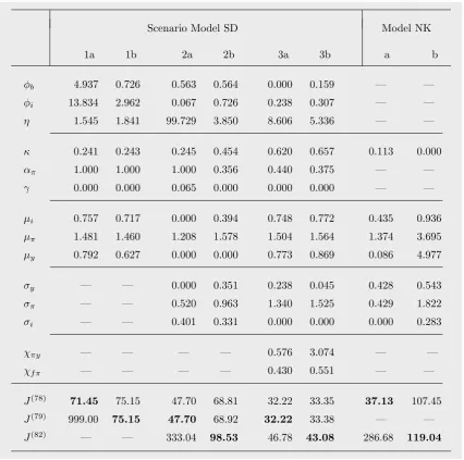
notation) was shown to exist that ensure uniqueness of this equilibrium, render it locally repelling, and give rise to a unique and globally attractive limit cycle. This feature carries over to the present formulation in discrete time and the slightly more general Taylor rule (9). Such a limit cycle can be viewed as the model’s representative business cycle.28 Our first MSM estimation then searches for a numerical parameter combination such that the 78 autocovariances from the list in (4) that it induces are as close as possible to their empirical counterparts. The solution of the corresponding minimization problem (1) with J =J(78) is reported as Scenario SD–1a in Table 1.
Before trying to assess whether a minimal loss of J(78) = 71.45 is more indicative of
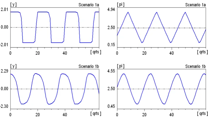
a good or a bad match, we should have a look at the cycles thus generated. The time series of the output gap yt and the inflation rate πt are shown in the upper two panels
in Figure 1. With a bit of more than five years, they may perhaps exhibit acceptable amplitudes and an acceptable period, but the pattern of the cyclical motions is clearly unsatisfactory. Output in reality simply does not crawl along a ceiling for roughly two years, then suddenly drops down on a floor and proceeds creeping there for another two years. It is thus also superfluous to comment on the tent-shape pattern of the inflation rate.
Responsible for this behaviour is the fact that the constraints in the transition prob-abilities, prob−+
t ,prob+
−
t ≤ 1 in (12), become binding over these stages. If we look at
the specification of the feedback index ft in eq. (13) then, owing to the high values of
the (stabilizing) coefficientφi on the real rate of interest and the (destabilizing) herding
coefficient φb, ft actually becomes so large in modulus that it takes quite a while for
it to return to more moderate values; and if it eventually does, it only takes two or three quarters until, with signs reversed, ft soars to similarly high levels again. Apart
from the unrealistic time series pattern, the resulting extreme probabilities are not very convincing, either.
These observations suggest introducing an additional moment m79 into the objective
function for the estimations. It considers the, as we may call them, “excess transition probabilities”αb exp(±ft) −1 from (12) and penalizes the occurrence of positive values
28To be more precise, there is a unique one-dimensional manifold P in the three-dimensional space towards which all (non-degenerate) trajectories converge in the sense that they move onP
Scenario Model SD Model NK
1a 1b 2a 2b 3a 3b a b
φb 4.937 0.726 0.563 0.564 0.000 0.159 — —
φi 13.834 2.962 0.067 0.726 0.238 0.307 — —
η 1.545 1.841 99.729 3.850 8.606 5.336 — —
κ 0.241 0.243 0.245 0.454 0.620 0.657 0.113 0.000
απ 1.000 1.000 1.000 0.356 0.440 0.375 — —
γ 0.000 0.000 0.065 0.000 0.000 0.000 — —
µi 0.757 0.717 0.000 0.394 0.748 0.772 0.435 0.936
µπ 1.481 1.460 1.208 1.578 1.504 1.564 1.374 3.695
µy 0.792 0.627 0.000 0.000 0.773 0.869 0.086 4.977
σy — — 0.000 0.351 0.238 0.045 0.428 0.543
σπ — — 0.520 0.963 1.340 1.525 0.429 1.822
σi — — 0.401 0.331 0.000 0.000 0.000 0.283
χπy — — — — 0.576 3.074 — —
χf π — — — — 0.430 0.551 — —
J(78) 71.45 75.15 47.70 68.81 32.22 33.35 37.13 107.45
J(79) 999.00 75.15 47.70 68.92 32.22 33.38 — —
J(82) — — 333.04 98.53 46.78 43.08 286.68 119.04
Table 1: Estimations of models SD and NK (Great Inflation).
Note: Bold face figures indicate the type of loss function for which the scenario is optimal. High values ofJ(79)are truncated at 999. Underlying NK–a, NK–b and the four stochastic scenarios of SD is the same random seed ¯c: among 1000 estimations with different random seeds, this ¯c
yields the median lossJ(82) for Scenario 3b.
so heavily that the loss minimization procedure better seeks to avoid them, even at the cost of a worse match of the other 78 moments. Formally we proceed in three steps. First, m79 is specified as the average excess transition probability over the simulation
horizonS (with respect to a given time path of the feedback indexft, which in turn, of
Figure 1: Time series yt, πtresulting from Scenario SD–1a and SD–1b.
weighting matrix W, for which a value of 1000 turns out to be perfectly suitable. Thus,
m79 = 1
S
S X
t=1
max{0, αb exp(ft)−1} + max{0, αb exp(−ft)−1}
mempT;79,79 = 0 (15)
W79,79 = 1000
The correspondingly augmented loss function is designated J(79),
J(79): loss function constituted by the 78 autocovariances and weights from (2), (4), plus momentm79 with weightW79,79 from (15)
(16)
Applying the new function J(79) to Scenario SD–1a quantifies its deficient time series features; the value we compute is so unacceptably high that in Table 1 we arbitrarily truncated it at 999.
The re-estimation of the deterministic model withJ(79), which forms our Scenario 1b,
confirms that the model can do better. As the table shows, adding the new criterion somewhat deteriorates the original matching, i.e. the lossJ(78)from the autocovariances
increases from 71.45 to 75.15. However, this seems a relatively low price for the total success concerning the excess transition probabilities, which have practically vanished (the 79th component of the loss is practically zero). Comparing the parameters in Sce-narios 1a and 1b it is seen that the general improvement is essentially brought about by considerably lower values of the two sentiment parametersφb and φi. They
the lower two panels of Figure 1. The slight asymmetry in the output gap proves that the nonlinearities in function (12) for the transition probabilities do take some effect in the outer regions of the state space.
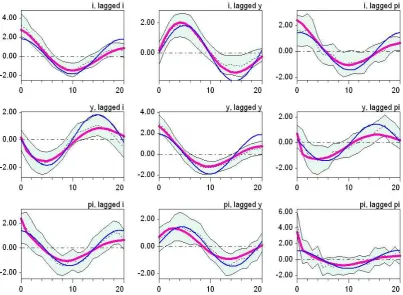
On this sound basis we can now ask what is behind the pure number of the minimized lossJ(79)= 75.15. Figure 2 presents the profiles of the nine auto- and cross-covariances of the three single variables it,yt, πt over a lag horizon of 20 quarters, which—it may
be taken into account—is longer than the eight quarters underlying the estimations themselves. The empirical covariances are given by the dotted lines with the shaded area of a 95% confidence band around them.29 The profiles generated by Scenario 1b
are plotted as the thin (blue) lines. At a glance and taking the confidence bands as a guideline, the matching can already be reckoned quite satisfactory. While there is a certain moderate tendency to leave the confidence band at the higher lags, within the first eight lags we observe only three cases with stronger deviations in this respect, all of which at a zero lag. That is, these are the simulated variances of the interest rate in the upper-left panel, of the output gap in the central panel, and of the inflation rate in the lower-right panel, where all of these moments are too low.
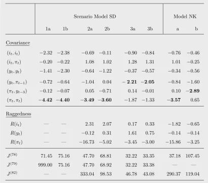
Table 2 reports selected t-statistics of our different estimations. With respect to Sce-nario 1b it shows that, in terms of this criterion, the first two “violations” are not very serious. The most critical point of the deterministic model is rather its inability to match the variance of the inflation rate or, more precisely, to trace out the sudden drop of Cov(πt, πt−h) from h= 0 to h= 1; since afterwards the changes in the autocovariances
remain relatively limited, the estimation decides to “sacrifice” the matching of the zero lag. It will have to be seen if the stochastic versions of the model can fare better in this respect.
As a secondary aspect we note in Table 2 that there is essentially one moment with which Scenario 1b pays for the more appropriate time series pattern vis-`a-vis Scenario 1a. This is the variance of the output gap with its deterioration toti =−2.30, which the
estimation of Scenario 1a had managed to keep inside the confidence interval. Regarding the autocovariances of the inflation rate, Scenario 1a and 1b share the same problem.
4.3. The simple stochastic version
In this subsection we activate the demand shocks εy,t in the output equation (7), the
cost push shocks επ,t in the Phillips curve (8), and the monetary policy shocks εi,t in
the Taylor rule (9). Hence the standard deviations σy, σπ, σi have to be estimated as
three additional parameters (the crossover effectsviaχπy andχf π are still switched off).
This also means that we have to choose a random seedc. As remarked on eq. (5) above,
Figure 2: Auto- and cross-covariance profiles of the sentiment dynamics (SD–1b) and (SD–3b) (GI).
Note: Thin (blue) lines indicate Scenario 1b, bold (red) lines Scenario 3b. Shaded areas are the bootstrapped 95% confidence bands around the empirical moments (dotted lines).
we adopt the same c = ¯c that will yield a median loss in our best estimation further below. The outcome from the minimization of our new loss functionJ(79) is reported as Scenario 2a in Table 1.
Comparing the loss J(79) = 47.70 to that of Scenario 1b, it is seen that the random
shocks can indeed achieve a nonnegligibly better match. More specifically, Table 2 with thet-statistics shows us a considerable improvement in the variances of the interest rate and the output gap, both of which are now inside the confidence intervals, and a more moderate improvement in the most critical moment, the variance of the inflation rate. Nonetheless, the latter is still clearly outside the confidence interval. Apart from that, note also that again there is no problem with excessively high transition probabilities as J(78)≈J(79) in Table 1.
If we look at the parameter estimates themselves, the extraordinarily high value of the proportionality factor η leaps to the eye. It is explained by the low value of φi
Scenario Model SD Model NK
1a 1b 2a 2b 3a 3b a b
Covariancge
(it, it) −2.32 −2.38 −0.69 −0.11 −0.90 −0.84 −0.76 −0.46 (it, πt) −0.20 −0.22 1.08 1.02 1.28 1.31 1.01 −0.25 (yt, yt) −1.41 −2.30 −0.64 −1.22 −0.37 −0.57 −0.34 −0.56 (yt, πt−1) −0.72 −0.64 −1.04 0.04 −2.21 −2.05 −0.84 −1.60 (πt, yt−3) −0.12 −0.07 0.05 −0.71 0.14 −0.01 0.10 −2.89 (πt, πt) −4.42 −4.40 −3.49 −3.60 −1.87 −1.33 −3.57 0.65
Raggedness
R(it) — — 2.31 2.07 0.17 0.33 −1.82 −0.65
R(yt) — — −0.12 0.31 1.61 0.75 −0.14 −0.14
R(πt) — — −16.73 −5.02 −3.45 −3.00 −15.86 −3.25
J(78) 71.45 75.16 47.70 68.81 32.22 33.35 37.18 107.45
J(79) 999.00 75.16 47.70 68.92 32.22 33.38 — —
J(82) — — 333.04 98.53 46.78 43.08 290.37 119.04
Table 2: Selected t-statistics of the estimations of models SD and NK (GI).
Note: Bold face figures indicate the most important shortcomings of the corresponding esti-mation.
extremely narrow fluctuations of the business climate bt(sinceft stays close to zero and
so prob−+
t and prob+
−
t in (11) differ only marginally). The high η then takes care that
the thus induced fluctuations of the output gap yt in eq. (7) are wide enough. While in
this way the motions of the observable variables may appear acceptable, the implausible behaviour of the nonobservable bt leaves an unpleasant aftertaste.
Instead of thinking about any immediate consequences of how to deal with this prob-lem, we widen the horizon for the empirical regularities that we want the model to repro-duce. The two middle panels in Figure 3 document the well-known fact that the empirical oscillations of the output gap yt as a level variable are relatively smooth, whereas the
sufficiently representative to illustrate that this scenario cannot account for the different time series patterns. It does not succeed in this respect even though the estimation gets along without any demand shocks (i.e.,σy= 0 in Table 1). The output gap is nevertheless
affected more indirectly by the monetary policy shocks, which take effect on the business climate viathe feedback index ft. They actually turn out to be so strong that the kind
of raggedness inytand πtlooks about the same. Thus, compared to the empirical series,
the simulatedyt seem to exhibit a similar degree of raggedness, and the simulatedπtare
clearly too smooth.
Figure 3: Empirical time series and yt, πt resulting from Scenarios 2a and 2b.
These verbal descriptions of what our eye perceives without further reflection lead us to
Clearly, this statistic is independent of the length and scale of the time series, and it can vary between unity and zero, indicating perfect raggedness and perfect smoothness, respectively. The indexN for the sample period T orS can be omitted in the following since it will be easily understood from the context.
As a time average, R(xt) is an ordinary summary statistic that can be effortlessly
added to the previous moments for a more ambitious moment matching. Also their variances can be bootstrapped from the empirical data in the same way as those in eq. (2) for our 78 autocovariances. Hence we may augment the present estimations by including the three moments
m80 = R(it), m81 = R(yt), m82 = R(πt) (18)
which gives rise to the loss functionJ(82),
J(82): loss function constituted byJ(79)plus moments m80, m81, m82
from (17) with their weights determined by (2) (19)
Endowed with a measure of raggedness, Table 2 now reassures us that the output gap in Scenario 2a displays an even perfect behaviour in this respect. The interest rate is less satisfactory, and the t-statistic of the inflation rate points out a serious failure.
The next question therefore is if the model can alleviate this mismatch by minimizing the augmented loss function J(82). The answer is given by the outcome of Scenario 2b. First of all, this estimation brings about a higher degree of raggedness for the inflation rate, although it is still markedly lower than in empirical inflation. On the other hand, the raggedness initandytis similar to Scenario 2a (see Table 2 and the illustration in the
two bottom panels in Figure 3). Unfortunately, this improvement comes at the cost of a sizeable deterioration in the matching of the autocovariances, withJ(78)= 68.81 versus
47.70 for Scenario 2a. Actually, Scenario 2b thus falls back to a level that is not very much better than in the deterministic model version. The deterioration is a relatively general phenomenon; there is no single moment that is mainly responsible for it (this does not only hold for the few moments shown in Table 2). In addition, the slightly higher value of J(79) versus J(78) for SD–2b indicates rare cases where the transition
probabilities prob−+
t or prob+
−
t hit their upper bound.
Turning to the estimated parameters in Table 1, we see a couple of differences from the previous estimations. First and most importantly, the high value in Scenario 2a forη
30Strictly speaking, the notationR
and the low value value forφiwith their dubious implications for the sentiment dynamics
do not carry over. Second, the slope parameter κ in the Phillips curve, which was very stable in the first three scenarios, has almost doubled. This goes along with a structural change in the adaptive inflation climate entering the Phillips curve. Before, we hadαπ= 1
and γ ≈0, so that the climate was (nearly) equal to the rate of inflation most recently observed,πc
t+1=πt, whereas now, withαπ ≈1/3, its adjustments occur in a truly gradual
manner. The credibility coefficientγ of the central bank remains nevertheless zero. Third, Scenario 2b has a moderate interest rate smoothing in the Taylor rule versus
no smoothing, µi= 0, in Scenario 2a and considerably stronger smoothing in the
deter-ministic cases. The zero responsiveness of the interest rate to output is maintained (even though it is again in stark contrast to the deterministic cases). Fourth, the present esti-mation differs from Scenario 2a in that it can no longer do without random perturbations on the demand side (σy >0), and it also requires stronger effects of the cost post shocks.
In sum, as far as the simple stochastic model is concerned, these features render Scenario 2b more trustworthy than Scenario 2a.
4.4. The stochastic version with crossover shock effects
Although Scenario 2b is more satisfactory than Scenario 2a, can we be happy enough with its overall goodness-of-fit? Instead of further meditating on this question, we postpone it. We rather take a next step and augment the model by admitting the crossover random shock effects. That is, we add the coefficients χπy in (10) and χf π in (13) to the list
of the parameters. This gives us model version SD–3 and a total of 14 parameters to estimate. We alternatively employ the loss functions J(79) and J(82), without and with the attempted matching of the raggedness in it,yt,πt, the minimization of which gives
rise to Scenario 3a and 3b, respectively.
The corresponding two columns in Table 1 reassure us that both coefficients χπy
and χf π come out with the correct positive sign, and they testify to a (very) strong
improvement of these two estimations over the simple stochastic version of the model. The two parameters are also both remarkable in that the much better match of the autocovariances that they produce simultaneously implies a good match of the raggedness statistics, too. That is, as evidenced by the small difference inJ(79)for Scenario 3a and 3b,
now only a very low price has to be paid in terms of a deterioration of the autocovariances if the model is additionally desired to reproduce the raggedness of the empirical time series.
Comparing the profiles of the autocovariances from Scenario 3b to those of the deter-ministic Scenario 1b in Figure 2, it can generally be stated that the former remain over longer lags in the empirical confidence bands, even though the estimation itself with its lag horizon of 8 quarters has not called for that. The most important achievement ofχπy