W O R K I N G PA P E R S E R I E S
N O . 5 1 0 / A U G U S T 2 0 0 5
FACTOR ANALYSIS
IN A NEW-KEYNESIAN
MODEL
In 2005 all ECB publications will feature a motif taken from the
€50 banknote.
W O R K I N G P A P E R S E R I E S
N O . 5 1 0 / A U G U S T 2 0 0 5
This paper can be downloaded without charge from http://www.ecb.int or from the Social Science Research Network electronic library at http://ssrn.com/abstract_id=750790.
FACTOR ANALYSIS
IN A NEW-KEYNESIAN
MODEL
1by Andreas Beyer,
2Roger E. A. Farmer,
3Jérôme Henry
4© European Central Bank, 2005 Address
Kaiserstrasse 29
60311 Frankfurt am Main, Germany
Postal address Postfach 16 03 19
60066 Frankfurt am Main, Germany
Telephone +49 69 1344 0
Internet http://www.ecb.int
Fax
+49 69 1344 6000
Telex 411 144 ecb d
All rights reserved.
Reproduction for educational and non-commercial purposes is permitted provided that the source is acknowledged.
C O N T E N T S
Abstract 4
Non-technical summary 5
1 Introduction 7
2 Single equation versus system approach 10
3 Robustness analysis 18
4 Enlarging the information set 21
4.1 The factor model 22
4.2 The role of the estimated factors 24 5 An analysis of identification and determinacy 25
5.1 An analysis of identification 25
5.2 An analysis of determinacy and
indeterminacy 28
6 33
References 35
39 44 51 Conclusions
European Central Bank working paper series Appendix A
Abstract
New-Keynesian models are characterized by the presence of ex-pectations as explanatory variables. To use these models for policy evaluation, the econometrician must estimate the parameters of expec-tation terms. Standard estimation methods have several drawbacks, including possible lack of identification of the parameters, misspecifi
-cation of the model due to omitted variables or parameter instability, and the common use of inefficient estimation methods. Several au-thors have raised concerns over the validity of commonly used instru-ments to achieve identification. In this paper we analyze the practical
relevance of these problems and we propose remedies to weak identifi
-cation based on recent developments in factor analysis for information extraction from large data sets. Using these techniques, we evaluate the robustness of recentfindings on the importance of forward looking
components in the equations of the New-Keynesian model.
JEL-Classification: E5, E52, E58
Key-words: New-Keynesian Phillips curve, forward looking
Non-technical Summary
This paper is about the estimation of New-Keynesian models of the mon-etary transmission mechanism. We evaluate a number of recent findings
obtained using single equation methods and we develop a system approach that makes use of additional identifying information extracted using factor analysis from large data sets.
A number of authors have used instrumental variable methods to estimate one or more equations of the New-Keynesian model of the monetary trans-mission mechanism. They used the New-Keynesian paradigm to explain the behavior of U.S. inflation as a function of its lag(s), expected lead(s), and the
marginal cost of production or the output gap. This work stimulated consid-erable debate, much of which has focused on the size and significance of future
expected inflation in the New-Keynesian Phillips curve. Similar arguments
have been made over the role of expected future variables in other equations of the New-Keynesian model such as Taylor rules in which expected future inflation appears as a regressor or models of the Euler equation for output in
which expected future output appears on the right-hand-side. The estimation of models that include future expectations has revived a debate that began in the 1970’s with the advent of rational expectations econometrics. The recent empirical literature on the New-Keynesian Model and in particular on estimating the New-Keynesian Phillips curve has highlighted four main problems with the single equation approach to estimation by GMM. First, parameter estimates may be biased due to correlation of the instruments with the error term. Second, an equation of interest could be mis-specified because
of omitted variables or parameter instability within the sample. Third, para-meters of interest may not be identified. Fourth, parameters may be weakly
argue, in this paper, that these issues can only be resolved by embedding the individual single equation models in a fully specified structural model.
We analyze the practical relevance of these problems, propose remedies for each of them, and evaluate whether the findings on the importance of the
forward looking component are robust when obtained within a more general econometric context. First we compare single equation and system methods of estimation for models with forward looking regressors. We then conduct a robustness analysis for a full forward looking system. In extending the information set we analyze the role of information extracted from large data sets to reduce the risk of specification bias and weak instruments problems.
Finally we conduct a formal analysis of identification and of issues related to
use of additional identifying information extracted using factor analysis from large data sets.
Following the influential work of Galí and Gertler (1999, GG), a number
of authors have used instrumental variable methods to estimate one or more equations of the New-Keynesian model of the monetary transmission mech-anism. GG used the New-Keynesian paradigm to explain the behavior of U.S. inflation as a function of its first lag, expected first lead, and the
mar-ginal cost of production. Their work stimulated considerable debate, much of which has focused on the size and significance of future expected inflation
in the New-Keynesian Phillips curve. Similar arguments have been made over the role of expected future variables in the other equations of the New-Keynesian model: for example Clarida, Galí and Gertler (1998) estimate a Taylor rule in which expected future inflation appears as a regressor and
Fuhrer and Rudebusch (2002) have estimated an Euler equation for output in which expected future output appears on the right-hand-side.
The estimation of models that include future expectations has revived a debate that began in the 1970’s with the advent of rational expectations econometrics. In this context, a number of authors have raised economet-ric issues that relate to the specification and estimation of single equations
with forward looking variables. For example, Rudd and Whelan (2001, RW) showed that the GG parameter estimates for the coefficient on future inflation
may be biased upward if the equation is mis-specified due to the omission of
relevant regressors that are instead used as instruments. With regard to the estimation of the coefficients of future variables they pointed out that this
1
Introduction
This paper is about the estimation of New-Keynesian models of the monetary transmission mechanism. We evaluate a number of recent findings obtained
variable from the right-hand-side and substitutes an infinite distributed lag
of all future expected forcing variables. RW use their analysis to argue in favor of Phillips curve specifications that favor backward lags of inflation over
the New-Keynesian specification that includes only expected future inflation
as a regressor.
Galí, Gertler and Lopez-Salido (2003, GGLS) have responded to the RW critique by pointing out that, in spite of the theoretical possibility of omitted variable bias, estimates obtained by direct and indirect methods are fairly close, and when additional lags of inflation are added as regressors in the
structural model to proxy for omitted variables, they are not significant.
While the Rudd-Whelan argument is convincing, the CGLS response is less so since other (contemporaneous) variables might also be incorrectly omitted from the simple GG inflation equation. Even if additional lags of inflation
were found to be insignificant, their inclusion could change the parameters
of both the closed form solution and the structural model. We argue, in this paper, that these issues can only be resolved by embedding the single equation New-Keynesian Phillips curve in a fully specified structural model.
Other authors, e.g. Fuhrer and Rudebusch (2002), Lindé (2003) and Jon-deau and Le Bihan (2003) have pointed out that the Generalized Method of Moment (GMM) estimation approach followed by GG could be less robust than maximum likelihood estimation (MLE) in the presence of a range of model mis-specifications such as omitted variables and measurement error,
typically leading to overestimation of the parameter of future expected infl
a-tion. GGLS correctly replied that no general theoretical results are available on the relative merits of GMM and MLE under mis-specification, that the
problem can yield differences between estimates that are based on the follow-ing two alternative estimation methods. The first (direct) method estimates
paper we hope to shed additional light on the efficiency and possible bias of GMM estimation by comparing alternative estimation methods on the same
data set and the same model specification.
A different and potentially more problematic critique of the GG approach comes from Mavroeidis (2002), Bårdsen, Jansen and Nymoen (2003), and Na-son and Smith (2003), building upon previous work on rational expectations by Pesaran (1987). Pesaran (1987) stressed that the conditions for identifi
-cation of the parameters of the forward looking variables in an equation of interest should be carefully checked prior to single equation estimation. To check identification conditions one must specify a model for all of the
right-hand-side variables. The articles cited above have shown that in a variety of alternative models, sensible specifications for the right-hand-side variables
lead to underidentification of the parameters of forward looking variables.
In the presence of underidentification, estimation by GMM yields unreliable
results.
Afinal and related argument against the indiscriminate use of single
equa-tion GMM estimaequa-tion of forward looking equaequa-tions relates to the quality of the instruments. This issue is distinct from that of underidentification since
an equation may be identified, but the instruments may be weakly correlated
with the endogenous variables, see in particular Mavroeidis (2002) for an ap-plication to the GG case. When the instruments are not particularly useful for forecasting the future expected variable, the resulting GMM estimators suffer from weak identification, which leads to non-standard distributions for
the estimators that can yield misleading inference, see e.g. Stock, Wright and Yogo (2002) for a general overview on weak instruments and weak iden-ti cation.
mation by GMM. First, parameter estimates may be biased due to correlation of the instruments with the error term. Second, an equation of interest could be mis-specified because of omitted variables or parameter instability within
the sample. Third, parameters of interest may not be identified. Fourth,
pa-rameters may be weakly identified if the correlation of the instruments with
the target is low.
In this paper we analyze the practical relevance of these problems, propose remedies for each of them, and evaluate whether the findings on the
impor-tance of the forward looking component are robust when obtained within a more general econometric context. In Section 2 we compare single equation and system methods of estimation for models with forward looking regres-sors. In Section 3 we conduct a robustness analysis for a full forward looking system. In Section 4 we analyze the role of information extracted from large data sets to reduce the risk of specification bias and weak instruments
prob-lems. In Section 5 we conduct a formal analysis of identification issues. In
Section 6 we summarize the main results of the paper and conclude.
2
Single Equation versus System Approach
We begin this Section with a discussion of the estimation of the New-Keynesian Phillips curve. This will be followed by a discussion of single-equation esti-mation of the Euler equation and the policy rule. We then contrast the single equation approach to a closed, three-equation, New-Keynesian model. We es-timate simultaneously a complete structural model which combines the three previously estimated single-equation models for the Phillips curve, the Euler equation and the policy rule and we compare system estimates of parameters with those of the three single-equation specifications.
esti-spired by the work of Galí and Gertler (GG 1999),
πt=α0+α1πet+1+α2xt+α3πt−1 +et, (1)
where πt is the GDP deflator, πet+1 is the forecast of πt+1 made in period t, xt is a real forcing variable (e.g. marginal costs as suggested by GG,
unemployment - with reference to Okun’s law - as in e.g. Beyer and Farmer (2003), or any version of an output gap variable). The error term et is
assumed to be i.i.d. (0, σ2
e) and is, in general, correlated with the
non-predetermined variables (i.e, with πe
t+1 and xt). Since we want to arrive
at the specification of a system of forward looking equations, we prefer to
use as a real forcing variable the unemployment rate or the output gap1,
measured as the deviation of real GDP from its one-sided HPfiltered version
as widely used in the literature.
To estimate equation (1) we replaceπe
t+1 withπt+1, such that (1) becomes πt =α0+α1πt+1+α2xt+α3πt−1+vt. (2)
Equation (2) can be estimated by GMM, with HAC standard errors to take into account the MA(1) structure of the error termvt=et+α1(πet+1−πt+1).2
All data is for the US, quarterly, for the period 1970:1-1998:4, where the constraint on the end date is due to the large data set we use in Section 4.
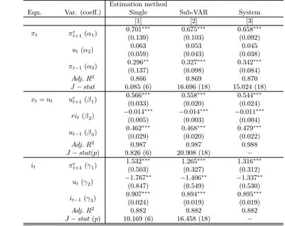
In the first panel of the first column of Tables 1 and 2 we report the
single-equation estimation results. In Table 1 xt represents unemployment 1The forward looking IS curve is usually speci
fied in terms of the output or
unemploy-ment gap.
2In particular, to compute the GMM estimates we start with an identity weighting
matrix, get afirst set of coefficients, use these to update the weighting matrix andfinally
iterate coefficients to convergence. To compute the HAC standard errors, we adopt the Newey West (1997) approach with a Bartlett kernel andfixed bandwidth. These
calcula-tions are carried out with Eviews 5.0.
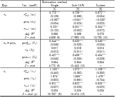
in-and in Table 2 it represents the output gap. As in GG (1999) in-and Galí et al. (2003), we find a larger coefficient on πe
t+1, about0.70, than on πt−1, about
0.30. The coefficient on the forcing variable is very small and not statistically significant at the 5% level, again in line with previous results.
There are at least two problems with this single equation approach: first,
the validity of the instruments cannot be evaluated and, second, the degree of over, just, or under-identification is undefined.
The issue of identification and the use of valid instruments in rational
expectations models is a very subtle one, see e.g. Pesaran (1987), Mavroeidis (2002) or Bårdsen et al. (2003). In linear backward looking models, such as conventional simultaneous equation models, rank and order conditions can be applied in a mechanical way (see e.g. Fisher, 1966). In rational expectation models, however, the conditions for identification depend on the
solution of the model, i.e. whether the solution of the model is determinate or indeterminate.
In our case, as it is common in this literature, we have used (three) lags of πt, xt and the interest rate, it as instruments where it is the 3-month US
Federal funds interest rate. However, since it does not appear in (1), both
πe
t+1 and xt may not depend on lags of it, which would make it useless as
an instrument. To evaluate whether or not lagged interest rates are suitable instruments, we estimated the following sub-VAR model:
xt = b0 +b1πt−1+b2xt−1+b3it−1+uxt,
it = c0+c1πt−1+c2xt−1+c3it−1+uct, (3)
whereuxt anduct are i.i.d. error terms, which are potentially correlated with
et. If b3 = 0, i.e., it does not Granger cause xt, then lags of it are not valid
instruments for the endogenous variables in (1).
one (i.e., πt−2, πt−3, xt−2 and xt−3) are valid instruments for πet+1 is also
questionable. If the solution for πt only depends onπt−1 andxt−1, which is
the case when the solution is determinate, then the additional lags are not valid instruments. However, in case of indeterminacy additional lags of πt
and xt matter, which re-establishes the validity of πt−2, πt−3, xt−2 and xt−3
as instruments. More details on this issue are provided in Section 5.
In the - for identification - “worst case” scenario of a determinate solution
and b3 = 0 in (3), we are left with only xt−1 as a valid instrument for πet+1
and xt (since πt−1 is a regressor in (1)), so that the structural equation is
underidentified. With a determinate solution and b3 6= 0, both xt−1 and it−1 are valid instruments for πet+1 and xt, which makes the model exactly
identified. With an indeterminate solution and b3 = 0, πt−2, πt−3, xt−1, xt−2 and xt−3 are in general valid instruments because often it is possible
to find an equivalent transformation of the rational expectations solution
that is free of expectations variables. Instead the solution has a higher order of dynamics, i.e. longer lags in the predetermined variables and moving average errors. (see e.g. Beyer and Farmer (2005)). In that case there are three overidentifying restrictions. Finally, with an indeterminate solution andb3 6= 0,πt−2,πt−3,xt−1, xt−2,xt−3,it−1,it−2 andit−3 are in general valid
instruments, which leads to six overidentifying restrictions.
As a consequence of the model dependence with respect to the number of valid instruments , the Hansen’sJ-statistic, a popular measure for the va-lidity of the instruments and overidentifying restrictions that we also present for conformity to the literature, can be potentially uninformative and even misleading when applied in a forward looking context.
Estimating (1) and (3) using only one lag of π, x, and i as instruments,
wefind thatb3 6= 0but the null hypothesisb3 = 0cannot be rejected. In this
resulting GMM estimators can suffer from weak identification. This might
lead to non-standard distributions for the estimators and can yield misleading inference, see e.g. Stock, Wright and Yogo (2002). Empirically, we find that
the size of the standard errors for the estimators of the parameters α1 and α2 in (1) matches the estimated values for α1 andα2.
However, when we estimate (1) and (3) using three lags ofπ, x, and ias
instruments, we find that b3 6= 0 but the null hypothesis b3 = 0 is strongly
rejected. The estimated parameters for (1) are reported in the first panel
in column 2 of Tables 1 and 2. Compared with the corresponding single equation estimates we find that the point estimates of the parameters are
basically unaffected (there is a non-significant decrease of about 5% in the
coefficient ofπe
t+1 and a corresponding increase in that ofπt−1). Yet, there is
a substantial reduction in the standard errors of 30-40%. Similar results are obtained when (3) is substituted for a VAR(3) specification. These findings
suggest that the model is identified, but the solution could be indeterminate.
Intuitively, indeterminacy arises because the sum of the estimated parameters
α1 andα3 in (1) is very close to one; a more formal analysis of identification
is provided in Section 5.
So far the processes for the forcing variables was assumed to be purely backward looking. As an alternative we consider a forward looking model also for xt. For example, Fuhrer and Rudebusch (2002) estimated a model
for a representative agent’s Euler equation (in their notation)
xt=β0+β∗1xet+1+β∗2(
1
k
k−1
X
j=0
(iet+j−πet+j+1)) +β∗3xt−1+β∗4xt−2+ηt, (4)
where xt is real output (detrended in a variety of ways), xet+1 is the forecast
of xt+1 made in periodt,it−πet+1 is a proxy for the real interest rate at time t, and ηt is an i.i.d. (0, σ2
η) error term. In our sample period, the second lag
model becomes
xt=β0+β1xet+1+β2(it−πet+1) +β3xt−1+ηt, (5)
and for x we use, again, either unemployment, or the GDP gap. Replacing the forecast with its realized value, we get
xt =β0+β1xt+1+β2(it−πt+1) +β3xt−1 +µt, (6)
where µt=β1(xe
t+1−xt+1) +β2(πet+1−πt+1).
As in the case of the New-Keynesian Phillips curve, this equation can be estimated by GMM, appropriately corrected for the presence of an MA component in the error term µt. As in our estimates of the New-Keynesian
Phillips curve, we use three lags of x, i and π as instruments. The results
are reported in the first column of the second panel of Table 1 (for xt as
the unemployment rate) and Table 2 (for xt as the output gap). In both
cases the coefficient on xe
t+1 is slightly larger than 0.5 and significant, and
the coefficient on xt−1 is also close to 0.5 and significant. These values are
in line with those in Fuhrer and Rudebusch (2002), who found lower values when using ML estimation rather than GMM and the positive sign of the real interest in the equation for the output gap is similar to the Fuhrer-Rudebusch results when they used HP de-trending.
As with the New-Keynesian Phillips curve, we estimate Equation (6) si-multaneously together with a sub-VAR(1) as in (3), but here for the forcing variables πt and it. Again, the significance of the coefficients in the VAR(1)
equations (in particular those for lagged πt in theit equation) lends support
In order to complete our building blocks for a forward looking system we
finally also model the interest rate with a Taylor rule as in Clarida, Galí and
Gertler (1998, 2000). Our starting point here is the equation
i∗t =i+γ1(πet+1−π∗t) +γ2(xt−x∗t), (7)
where i∗
t is the target nominal interest rate, i is the equilibrium rate, xt is
real output, and π∗t and x∗t are the desired levels of inflation and output.
The parameter γ1 indicates whether the target real rate adjusts to stabilize
inflation (γ1 > 1) or to accommodate it (γ1 < 1), while γ2 measures the concern of the central bank for output stabilization.
Following the literature, we introduce a partial adjustment mechanism of the actual rate to the target rate i∗ :
it= (1−γ3)i∗t +γ3it−1 +vt, (8)
where the smoothing parameter γ3 satisfies 0 ≤ γ3 ≤ 1, and vt is an i.i.d.
(0, σ2
v)error term. Combining (7) and (8), we obtain
it =γ0+ (1−γ3)γ1(πet+1−π∗t) + (1−γ3)γ2(xt−x∗t) +γ3it−1+vt (9)
where γ0 = (1−γ3)i, which becomes
it =γ0+ (1−γ3)γ1(πt+1−π∗t) + (1−γ3)γ2(xt−x∗t) +γ3it−1+ t, (10)
with t= (1−γ3)γ1(πet+1−πt+1) +vt, after replacing the forecasts with their
realized values
The results for single equation GMM estimation (with 3 lags as instru-ments) are reported in thefirst column of the third panel of Tables 1 and 2.
As in Clarida et al. (1998, 2000), the coefficient on future inflation is larger
Again, as in the cases of single equation estimations of the Phillips curve and the Euler equation, we are able to reduce the variance of our point estimates by adding sub-VAR(1) equations for the forcing variables πt and xt when
estimating the resulting system by GMM (see column 2). As above, for both approaches we have used up to three lags for the intrument variables.
We are now in a position to estimate the full forward looking system, composed of Equations (1), (5) and (9):
πt = α0+α1πet+1+α2xt+α3πt−1+et, (11)
xt = β0+β1xet+1+β2(it−πet+1) +β3xt−1+ηt,
it = γ0+ (1−γ3)γ1(πet+1−π∗t) + (1−γ3)γ2(xt−xt∗) +γ3it−1+vt
The results are reported in column 3 of Tables 1 and 2. For each of the three equations the estimated parameters are very similar to those obtained either in the single equation case or in the systems completed with VAR equations. Furthermore, the reductions in the standard errors of the estimated parame-ters are similar to those obtained with sub-VAR(1) specifications. Since the
VAR equations can be interpreted as reduced forms of the forward looking equations, this result suggests that completing a single equation of interest with a reduced form may be enough to achieve as much efficiency as within a full system estimation. However, the full forward looking system represents a more coherent choice from an econometric point of view, and the finding
that the forward looking variables have large and significant coefficients in
all the three equations lends credibility to the complete rational expectations model.
The nonlinearity of our system of forward looking equations makes the evaluation of global identification impossible. However, if we linearize the
model around the estimated parameters and focus on local identification, we
identi-fied. Exact identification holds when the point estimates imply a
determi-nate solution. The model would be potentially overidentified in case of an
indeterminate equilibrium.
3
Robustness analysis
While system estimation increases efficiency, the full forward looking model in (11) could still suffer from mis-specification problems. To evaluate this
possibility, we conducted four types of diagnostic tests. First, we ran an LM test on the residuals of each equation to check for additional serial correlation i.e. serial correlation beyond the one that is due to the MA(1) error struc-ture of the model. Second, we ran the Jarque and Bera normality test on the estimated errors. Although our GMM estimation approach is robust to the presence of non-normal errors,3 rejection of normality could signal other
problems, such as the presence of outliers or parameter instability. Third, we ran an LM test to check for the presence of ARCH effects; rejection of the null of no ARCH effects might more generally be a signal of changes in the variance of the errors. Finally, we checked for parameter constancy by running recursive estimates of the forward looking system.
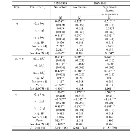
The results of our mis-specification tests are reported in the bottom lines
of each panel in Tables 3 and 4. For convenience, we also present in column 1 again the estimated parameters. When unemployment is used (Table 3) there are only minor problems of residual correlation in the inflation equation, but
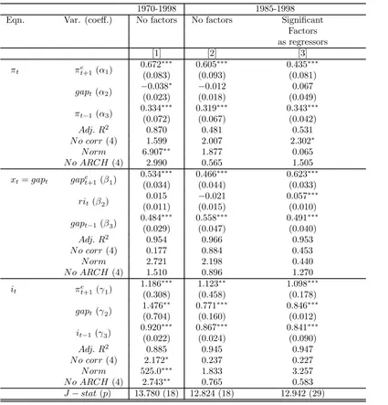
normality and no ARCH are strongly rejected in all of the three equations. The outcome of the tests is slightly better with the GDP gap (Table 4), but normality is still strongly rejected for the inflation and interest rate
equations, and the interest rate equation also fails the test for absence of
3Note that this is not the case for maximum likelihood estimation.
The rejection of correct specification could be due to parameter instability
in the full sample 1970:3 - 1998:4. Instability might be caused by a variety of sources including external events such as the oil shocks, internal events, such as the reduction in the volatility of output (e.g. McConnell and Perez-Quiros (2000)), or changes in the monetary policy targets. Since we had more faith in the second part of our sample, we implemented a backward recursion by estimating the system first for the subsample 1988:1-1998:4, and recursively
reestimating the system by adding one quarter of data to the beginning of the sample, i.e. our second subsample consisted of the quarters 1987:4—1998:4, our third was 1987:3 — 1998:4 and so on until 1970:3-1998:4.
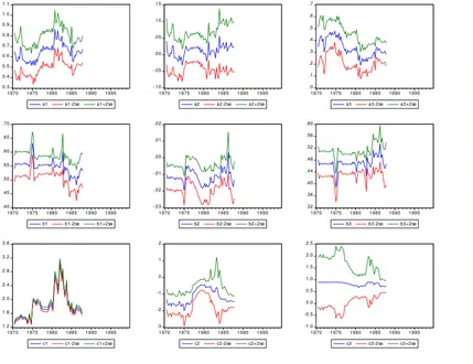
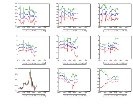
In Figures 1 and 2, we report recursive parameter estimates. These fi
g-ures confirm that the likely source of the rejection of ARCH, normality and
serial correlation tests is the presence of parameter change. Although the pa-rameter estimates are stable back to 1985:1, going further back than this is associated with substantial parameter instability in all three equations, and particularly in the estimated Taylor rule. Although parameter instability is more pronounced when we use unemployment as a measure of economic activity, it is also present in estimates obtained when using the output gap.
Overall, these mis-specification tests cast serious doubts on results
ob-tained for the full sample, and they suggest that a prudent approach would be to restrict our analysis to a more homogeneous sample. For this reason, in the subsequent analysis, we report results only for the subperiod 1985:1-1998:4.
coefficients of the Taylor rule differ substantially from the single equation estimates. Table 3 shows that (using unemployment as a measure of economic activity) restricting parameter estimates to the post 1985 subsample caused the estimated coefficient on future inflation to increase substantially. Table
4, (using the output gap) shows instead a marked decrease in the estimated coefficient on the output gap. In the post 1985 subsample we fail to reject the null hypothesis for all four of our diagnostic tests, thereby lending additional credibility to our estimation results.
The final issue we briefly consider is the role of the method of
estima-tion. Fuhrer and Rudebusch (2002), Lindé (2003) and Jondeau and Le Bi-han (2003) have suggested that GMM may lead to an upward bias in the parameters associated with the forward looking variables, while maximum likelihood (ML) produces more robust results. In case of exact identification
ML coincides with indirect least squares. We compared our estimates with the point estimates from GMM by computing the indirect least squares esti-mates from the reduced form. Using this approach, we find that our GMM
estimates are similar to the ML values.
For the subsample 1985-1998, using unemployment as the activity vari-able, the estimated coefficient on πe
t+1 in the inflation equation is 0.73 and
that on uet+1 in the unemployment equation is 0.64. The corresponding
val-ues using GMM are 0.73and0.51. Using the output gap, the ML estimates
become 0.76for the coefficient on πe
t+1 in the inflation equation and0.62for
that on future expected output gap in the Euler equation whereas the GMM estimates of these parameters are, respectively,0.61and0.47. The differences are slightly larger for the coefficient on future inflation in the Taylor rule, in
the range 2.1−2.4 with ML. Overall we are reassured that our finding of
significant coefficients on future expected variables is robust to alternative
4
Enlarging the information set
The analysis in Sections 2 and 3 supports the use of a system approach to the estimation of forward looking equations. For the 1985:1—1998:4 sample, our estimated system passes a wide range of mis-specification tests. Moreover,
the Hansen’s J-statistic, reported at the foot of Tables 3 and 4, is unable to
reject the null of valid instruments for this period (but it is worth recalling the caveats on the use of theJ-test in this context). However, there could still
be problems of weak instruments and/or omitted variables which are hard to detect using standard tests, (see e.g. Mavroeidis (2002)). This section proposes a method that can potentially address both of these issues.
Our approach is to augment our data by adding information extracted from a large set of 146 macroeconomic variables as described in Stock and Watson (2002a, 2002b, SW). We assume that these variables are driven by a few common forces, i.e. the factors, plus a set of idiosyncratic shocks. This assumption implies that the factors provide an exhaustive summary of the information in the large dataset, so that they may alleviate omitted variable problems when used as additional regressors in our small system. Moreover, the factors extracted from the Stock and Watson data are known to have good forecasting performance for the macroeconomic variables in our small dataset and they are therefore likely to be useful as additional instruments that may alleviate weak instrument problems, too.
of factors in our analysis is that, the inclusion of factors in small scale VARs has been shown to remove the “price puzzle” suggesting that factors may be used to reduce or eliminate the estimation bias, that arises from the omission of relevant right-hand-side variables.4
In the following subsection, we present a brief overview on the specifi
ca-tion and estimaca-tion of factor models for large datasets. Following this discus-sion, we evaluate whether the use of the estimated factors changes the size and or the significance of the coefficients of the forward looking components
in the New Keynesian model.
4.1
The factor model
Equation (12) represents a general formulation of the dynamic factor model
zt=Λft+ξt, (12)
where zt is an N×1 vector of variables and ft is an r×1 vector of common
factors. We assume that r is much smaller than N, and we represent the
effects offtonztby theN×rmatrixΛ. ξitis anN×1vector of idiosyncratic
shocks.
Stock and Watson require the factors,ft, to be orthogonal although they
may be correlated in time and with the idiosyncratic components for each factor.5 Notice that the factors are not identified since Equation (12) can be
rewritten as
zt =ΛGG−1ft+ξt =Ψpt+ξt,
where pt is an alternative set of factors andGis an arbitrary invertibler×r
matrix. This fact makes it difficult to form a structural interpretation of the
4For a definition and discussion of this issue the reader is referred to Christiano,
Eichen-baum and Evans (1999) pages 97—100. 5Precise moment conditions on ftand ξ
t, and requirements on the loading matrix Λ,
factors, but it does not prevent their use as a summary of the information contained in zt.
SW define the estimatorsfbt as minimizing the objective function
VN,T(f,Λ) =
1
NT
N
X
i=1
T
X
t=1
(zit−Λift)2.
Under the hypothesis of r common factors, they show that the optimal
es-timators of the factors are the r eigenvectors corresponding to the r largest eigenvalues of the T ×T matrix N−1PN
i=1ziz 0
i, where zi = (zi1, ..., ziT).
Moreover, the r eigenvectors corresponding to the r largest eigenvalues of the N ×N matrix T−1PT
t=1ztz 0
t are the optimal estimators of Λ. These
eigenvectors coincide with the principal components of zt; they are also the
OLS estimators of the coefficients in a regression of zit on the k estimated
factors fbt, i = 1, ..., N.6 Although there are alternative estimation methods
available, we chose the SW approach since there is some evidence to suggest that it dominates the alternatives in this context.7
No statistical test is currently available to determine the optimal number of factors. SW and Bai and Ng (2002) suggested minimizing a particular information criterion, however its small sample properties in the presence of heteroskedastic idiosyncratic errors deserves additional investigation. In their empirical analysis with this data set, SW found that the first 2-3 factors are
6SW prove that when r is correctly specified, ftb converges in probability toft, up to an arbitrary r×r transformation matrix, G. When k factors are assumed, withk > r,
k−restimated factors are redundant linear combinations of the elements offt, while even
when k < r consistency for thefirstk factors is preserved (because of the orthogonality
hypothesis). See Bai (2003) for additional inferential results.
7Forni, Hallin Lippi and Reichlin (2000) have developed an alternative frequency
the most relevant for forecasting key US macroeconomic variables. In the following analysis we however evaluate the role of up to six factors to make sure sufficient information is captured.
4.2
The role of the estimated factors
As we mentioned, the estimated factors can proxy for omitted variables in the specification of the forward looking equations. In particular, we use up
to six contemporaneous factors as additional regressors in each of the three structural equations, and retain those which are statistically significant.
Since the factors are potentially endogenous, we use their first lag as
additional instruments. These lags are likely to be useful also for the other endogenous variables in each structural equation.
In column 3 of Table 3 we report the results of GMM estimation of the forward looking system over the period 1985-1998 using unemployment as the activity variable, and in column 3 of Table 4 those using the GDP gap.
First, a few factors are strongly significant in the equations for inflation
and the real variable. While it is difficult to provide an economic interpreta-tion for this result, it does point to the omission of relevant regressors in the Phillips curve and Euler equation. In contrast, no factors are significant in
the Taylor rule, which indicates that output gap and inflation expectations
are indeed the key driving variables of monetary policy over this period. Second, in general the estimated parameters of the forward looking vari-ables are 10 to 20% lower than those without factors, but they remain strongly statistically significant.
Third, the precision of the estimators systematically increases, as the standard errors of the estimated parameters are 10 to 50% lower than those without the factors. This confirms the usefulness of the additional
Fourth, since the highest lag order of the regressors in the structural model is one, it could suffice to include one lag of πt, xt, and it in the
instrument set instead of three lags. In this case, the point estimates are unaffected, as expected, but the standard errors increase substantially. This
finding suggests that the solution of the system could be indeterminate, in
which case more lags would indeed be required.
Finally, since there is no consensus on the best way to compute robust standard errors in this context, we verified the robustness of our findings
based on Newey West (1994) comparing them with those based on Andrews (1991). The latter are in general somewhat lower, but the advantages result-ing from the use of factors are still systematically present.
5
An analysis of identi
fi
cation and
determi-nacy
This section analyzes two issues that are related to the internal consistency of the New-Keynesian model studied in Sections 2 - 4; we study the iden-tification of the parameters in our estimated equations and we ask, given
our point estimates, if the implied system leads to a determinate economic model. The first is an econometric issue: Are the coefficients in each of our
three equations identified? The second is an economic issue: What is the
ap-propriate interpretation of our estimates for the conduct of monetary policy? We turn first, to the question of identification.
5.1
An analysis of identi
fi
cation
of forward looking models based on the earlier work of Pesaran (1987). These authors pointed out that GMM estimates of single-equation rational expec-tations models only make sense if the equations are identified. In this section
we provide a formal analysis of identification within a fully articulated
three-equation rational expectations model. As mentioned in Section 2, global identification for this model cannot be tested due to its non-linear specifi
-cation. But we can demonstrate that, under the given coefficient estimates, the model is locally identified. We introduce a notation for indexing each
equation within a matrix representation of the model. To this end, let Yt
= (πt, xt, it)0 be the vector of endogenous variables consisting of inflation,
a measure of economic activity (unemployment or the output gap) and the interest rate, respectively, and letEt(Yt+1)be the expectation of the
realiza-tion of Yt+1 under the assumption that the model is a correct representation
of the time series process for all of the endogenous variables. The models that we estimated in Sections 2 - 4 are three-equation structural models with
the form:
A
(3×3)(3Y×t1)
+ F
(3×3)Et(3[Y×t1)+1]
= B
(3×3)(3Yt×−1)1
+ Φ
(3×1)C+(3V×t1)
, (13)
which can be written more compactly as follows
h
A F
i⎡
⎣ Yt
Et[Yt+1]
⎤
⎦=BYt−1+ΦC+Vt, (14)
The matrices A and F contain coefficients of the endogenous variables Yt
and Et[Yt+1] and the matrix B represents coefficients of the predetermined
variables Yt−1. The termC represents a vector of constants. In the following analysis, we drop C and interpret the variables Yt and Yt−1 as deviations
from means.
Since Et[Yt+1] represent expectations formed at date t, they should be
endogenous variables; the three elements of the vector Yt plus the three
ex-pectations of Yt+1 at date t. To close the system we need three additional
equations which, under the rational expectations assumption, are provided by the forecast equations
Et−1[Yt]−Yt =Wt,
where the Wt are additional non fundamental errors that may or may not
be exact functions of the fundamental errors, Vt. Let us now check for local
identification in the determinate case. The solution of model (13) is:
Yt=ΠYt−1+ Vt.
In the determinate case the matrix Π is 3-by-3 and is identical to the
reduced form. Since
Yt+1 =ΠYt
and
AYt+FΠYt = BYt−1+Vt
(A+FΠ)Yt = BYt−1+Vt
(A+FΠ)ΠYt−1 = BYt−1+Vt
and therefore
(A+FΠ)Π=B. (15)
To fulfil the order condition for identification of the structural parameters
inA,Fand Bthe number of free structural parameters must not exceed the
number of parameters in Π. We have imposed the following restrictions on
the matrices A,F and B :
[A F B]
⎡ ⎢ ⎢ ⎢ ⎣
1 a12 a13= 0 f11 f12 = 0 f13= 0 b11 b12 = 0 b13= 0
a21= 0 1 a23 f21=−a23 f22 f23= 0 b21= 0 b22 b23= 0
a31= 0 a32 1 f31 f32 = 0 f33= 0 b31= 0 b32 = 0 b33
⎤ ⎥ ⎥ ⎥ ⎦
Row 1 of this matrix represents the New-Keynesian Phillips curve. The unit entry in the first column indicates that this equation is normalized on
inflation and the zero entry in the third column indicates that the interest rate
does not enter the equation. The other rows have similar interpretations. For example, row 2 which represents the Euler equation is normalized by setting the coefficient onxt to unity. The equality restriction, f21 =−a23, imposes
the same coefficient on the nominal interest rate and the negative of expected future inflation; in words, this restriction means that expected inflation and
the nominal interest rate only affect the Euler equation through their effect on the expected real interest rate. Notice that we have imposed exactly six linear restrictions in each equation which implies that, in each case, the order condition is exactly satisfied.
To check the rank condition locally we apply the inverse mapping theorem to equation (15) and take the total differential:
dA(Π) +AdΠ+dF(Π)(Π) +F dΠ(Π) +FΠdΠ = dB dA(Π) + (A+FΠ)dΠ+dFΠ2+F dΠ(Π) = dB.
We then solve for dA, dF and dB, given the fixed parameters of the
models estimated in Sections 2 - 4. We demonstrate in Appendix A that each
dA, dFanddB is a function only of fixedA,F,B andΠ and of changes in
the reduced formdΠbut not of changes in the structural parameters.
5.2
An analysis of determinacy and indeterminacy
the individual pieces must add up to a coherent whole that can be used to provide an economic explanation of the causes of real-monetary interactions over the estimation period. The dominant current explanation provided by Clarida et. al. and substantiated by Boivin and Giannoni (2003, BG) and Lubik and Schorfheide (2004, LS) is that in the period after 1980 the New-Keynesian model was driven by an active monetary policy that led to a determinate equilibrium. We summarize the concept of determinacy briefly
below. Following this summary, we study the dynamic properties of New-Keynesian model when we replace theoretical coefficient values by our point estimates and we compare our results with those of CGG, BG and LS.
Since rational expectations have variables that are forward looking, the mapping from the structural to the reduced form is more complicated than in standard Cowles Commission econometrics. The reduced form of the model is a set of equations, one for each endogenous variable, that explains the time paths of each variable as a function of exogenous and predetermined variables. The mapping from the structural model to the reduced form may or may not be unique. It is also possible that no stationary reduced form exists. If the mapping is unique we say that the model is determinate; if it is non-unique the model is indeterminate and if no stationary solution exists the reduced form is non-existent.
The determinacy properties of our model may be analyzed byfirst writing
the system in its companion form;
More compactly,
A0
(6×6) Yt∗ (6×1)
= A1
(6×6) Yt∗−1 (6×1)
+ Pv
(6×3) Vt
(3×1)
+ Pw
(6×3) Wt
(3×1)
. (17)
Elements of the3×1vectorVtare called fundamental errors and the elements
of the 3×1 vector Wt are non-fundamental errors. The non-fundamental
errors may be functions of the fundamental errors or, if the model is indeter-minate, they may be independently determined. In this case they represent separate ‘sunspot’ shocks.
The reduced form of the model is found by choosing the expectations variables at date t to eliminate any unstable roots. This procedure may, or
may not, eliminate the influence of the endogenous errors,Wt and it leads to
a representation of the form
Yt∗ =AeY∗
t−1+P˜vVt+P˜wWt.
There are three possible cases to consider, all of which may occur in prac-tice. For the case when A0 is non-singular, these cases may be enumerated
by comparing the number of unstable roots of the matrix A−1
0 A1 with the
number of non-predetermined initial conditions. In the singular case, as oc-curs in our example, they involve a comparison of the generalized eigenvalues of(A0,A1)with the number of expectations of future endogenous variables.8
For our example there are three of these. If there are more than three un-stable generalized eigenvalues then no un-stable rational expectations solution exists. If there are exactly three unstable generalized eigenvalues then there is a unique rational expectations equilibrium and the model is said to be de-terminate. In this case the matrix Ae has rank 3 and P˜w is identically zero. 8For a description of how the Schur decomposition can be used to solve linear rational
If there arem <3unstable generalized eigenvalues thenAe has rank(6−m), ˜
Pw has rankm and the model is said to possess m degrees of indeterminacy.
In this last case the model can be closed by specifying a given covariance matrix for [Vt, Wt]and interpreting the Wtas non-fundamental, or ‘sunspot’
shocks that may be correlated with the fundamentals. Table 5 summarizes the implications of our point estimates for the determinacy properties of the data generating process under alternative estimation schemes and alternative models. Starting with the model without factors, there seems to be either no stationary rational expectations equilibrium or an indeterminate equilibrium, depending on the estimation method. The result is robust to the adoption of either unemployment or the output gap as the scale variable.
The determinacy of a model is a property of the system as a whole and it is sensitive to the model specification.9 Following Clarida-Galí-Gertler
(1998), a number of authors have estimated systems or partial systems of equations similar to those in this paper and they have used these estimates to infer the determinacy properties of the U.S. data. A consistent conclusion that arises in this literature is that the data before 1980 appears consistent with an indeterminate equilibrium partly driven by sunspots and the data after 1980 is well characterized by a determinate equilibrium in which only fundamental shocks influence the data-generating-process.
Clarida-Galí Gertler (1998) estimate a policy rule and embed it into a calibrated model. Later, full system estimates by Boivin and Giannoni (2003) and Lubik and Schorfheide (2004) confirm these determinacyfindings. All of
these authors either impose the values of some of the key parameters or they
9Beyer and Farmer (2003a) conduct a systematic search of the parameter space in a
use Bayesian estimators in which parameter values are strongly influenced
by priors. A likely source of divergence of our results from theirs, is that we allow all of the parameters of the model to be freely estimated. Since our results contradict the received wisdom, we conducted a sensitivity analysis to investigate this conjecture.
One of the main differences of our estimates from those of previous lit-erature is the low estimated value of β2, the real interest rate coefficient in
the Euler Equation. Using the output gap as the scale variable led to an estimated value for β2 of−0.021. However, this estimate is highly imprecise
with a standard error of 0.015. Since β2 is a key parameter for the determi-nacy properties of the model, we checked these properties for values of the real interest rate parameter that were larger but still within two standard errors of the point estimate. When we increased the absolute value ofβ2 to
−0.03 (preserving the negative sign) we found that the model has a unique
determinate rational expectations equilibrium. For the case of unemploy-ment as a scale variable ourfindings were similar. In this case, the estimated
parameter has the wrong sign and although it is small, −0.006, the estimates are, in this case, more precise.10 However, by imposing a value for α2 of
+0.011, in line with economic theory, we were able to restore determinacy of equilibrium.11
As an alternative to a priori restricting the parameters, the use of factors as additional regressors and instruments can yield a determinate solution, at least in the case where unemployment is used as the real variable in the system, see the last column of Table 5.
We conclude from our study that evaluating the determinacy properties
10When unemployment is the scale variable, the sign of the real interest coefficient in the Euler equation is predicted to be positive rather than negative.
11Another way to achieve determinacy is to constraint the parameters ofxe
of our model is difficult since minor changes in the parameter values can move the solution from the unstable region to the determinate or even indetermi-nate regions. However, with few simple and reasonable constraints on the parameters, or using the factors, data after 1985 is not inconsistent with the New-Keynesian interpretation of a determinate equilibrium driven by three fundamental shocks. The estimated parameters of the complete model form a consistent picture which coincides with New-Keynesian economic theory.12
6
Conclusions
In this paper we provided a general econometric framework for the analysis of models with rational expectations, focusing in particular on the hybrid version of the New-Keynesian Phillips curve that has attracted considerable attention in the recent period.
First, we showed that system estimation methods where the New-Keynesian Phillips curve is complemented with equations for the interest rate and ei-ther unemployment or the output gap yield more efficient parameter esti-mates than traditional single equation estimation, while there are only minor changes in the point estimates and the expected future variables play an im-portant role in all the three equations. The latter result remains valid even if MLE is used rather than system GMM.
Second, we stressed that it is important to evaluate the correct specifi
ca-tion of the model, and we showed that our systems provide a proper statisti-cal framework for the variables over the 1985-1998 period, while during the
12We should note however, that the New-Keynesian explanation is one of many
’70s there is evidence of parameter changes, in particular in the interest rate equation.
Third, we analyzed the role of factors that summarize the information contained in a large data set of U.S. macroeconomic variables. Some factors were found to be significant as additional regressors in the New-Keynesian
Phillips curve and in the Euler equation, alleviating potential omitted vari-able problems. Moreover, using lags of the factors as additional instruments in our small New-Keynesian system, the standard errors of the GMM esti-mates systematically decrease for all the estimated parameters; the gains are particularly large for the coefficients of forward looking variables. In addition, the use of factors can influence the characteristics of the equilibrium.
Fourth, we demonstrated that our GMM procedures were well defined and
the equations we estimated are identified. The point estimates of our system
form a coherent whole that has dynamic properties that are similar to the systems estimated (and calibrated) by Clarida et. al., Boivin and Giannoni, and Lubik and Schorfheide. If we impose prior information, as to these earlier studies, wefind that the system after 1980 is associated with a unique
determinate equilibrium driven solely by shocks to fundamentals. However, we detected substantial uncertainty on the characteristics of the equilibrium, which suggests that existing interpretations of the data are fragile, and are sensitive to the priors of the researcher.
References
[1] Andrews, D.W.K. (1991), “Heteroscedasticity and Autocorrelation Con-sistent Covariance Matrix Estimation, Econometrica, 59, 817-858.
[2] Bai, J. (2003), “Inferential theory for factor models of large dimension”, Forthcoming in Econometrica.
[3] Bai, J. and S. Ng (2002), “Determining the number of factors in approx-imate factor models”, Econometrica, 70, 191-223.
[4] Bårdsen, G. Jansen, E.S. and R. Nymoen, (2003), “Testing the New-Keynesian Phillips curve,” Memorandum 18/2002, Oslo University.
[5] Benhabib, J. and R. E. A. Farmer (1999), “Indeterminacy and Sunspots in Macroeconomics” in Handbook of Macroeconomics Vol. 1A, Taylor, J
and M. Woodford eds., North Holland.
[6] Bernanke, B. and J. Boivin (2003), “Monetary policy in a data-rich environment”, Journal of Monetary Economics, 50(2), pp. 525-46.
[7] Beyer, A. and R.E.A. Farmer (2003a), “Identifying the monetary trans-mission mechanism using structural breaks”, European Central Bank Working Paper Series #275.
[8] Beyer, A. and R.E.A. Farmer (2003b), “On the indeterminacy of New-Keynesian economics”, European Central Bank Working Paper Series #323.
[10] Boivin, J. and M. Giannoni (2003), “Has monetary policy become more effective”, NBER Working Paper #9459.
[11] Christiano, L.J., Eichenbaum, M., and C.L. Evans (1999), “Monetary Policy Shocks: What have we learned and to what end?” in Handbook
of Macroeconomics Vol. 1A, Taylor, J and M. Woodford eds., North
Holland.
[12] Clarida, R. Galí, J., and M. Gertler (1998), “Monetary policy rules in practice: Some international evidence”,European Economic Review, 42,
1033-1067.
[13] Clarida, R., Galí, J., and M.Gertler (2000), “Monetary policy rules and macroeconomic stability: evidence and some theory”,Quarterly Journal
of Economics, 115, 147-180.
[14] Favero, C., Marcellino, M. and F. Neglia (2004), “Principal components at work: the empirical analysis of monetary policy with large datasets”,
Journal of Applied Econometrics, forthcoming.
[15] Fisher, F. (1966), The Identification Problem in Econometrics. New
York: McGraw-Hill.
[16] Forni, M., Hallin, M., Lippi, M. and L. Reichlin (2000), “The generalised factor model: identification and estimation”, The Review of Economic
and Statistics, 82, 540-554.
[17] Fuhrer, J.C. and G. D. Rudebusch (2002), “Estimating the Euler equa-tion for output”, Federal Reserve Bank of Boston, WP 02-3.
[18] Galí, J. and M. Gertler (1999), “Inflation Dynamics: A structural
[19] Galí, J., Gertler, M., and Lopez-Salido, J. D. (2003), “Robustness of the estimates of the hybrid New-Keynesian Phillips curve”, mimeo, Bank of Spain.
[20] Hamilton, J.D. (1994),Time series analysis Princeton University Press,
Princeton, NJ.
[21] Ireland, P.N. (2001), “Sticky price models of the business cycle:
Speci-fication and stability,” Journal of Monetary Economics, 47(1), 3-18.
[22] Jondeau É. and H. Le Bihan (2003), “ML vs GMM estimates of hy-brid macroeconomic models (with an application to the ‘New Phillips curve’)”, Banque de France, WP 103.
[23] Kapetanios, G. and M. Marcellino (2003), “A Comparison of estimation methods for dynamic factor models of large dimensions”, mimeo, IGIER, Bocconi University.
[24] Lubik, T. and F. Schorfheide (2004), “Testing for indeterminacy: An application to U.S. monetary policy”,American Economic Review, 94(1)
190—217.
[25] Lindé, J., (2003) “Estimating New-Keynesian Phillips curves: A full in-formation maximum likelihood approach,” Sveriges Riksbank, Working Paper No. 129.
[26] Mavroeidis, S. (2002), “Identification and mis-specification issues in
for-ward looking monetary models”, University of Amsterdam Econometrics Discussion Paper No. 2002/221.
[27] McConnell, M.M. and G. Perez-Quiros (2000) “Output fluctuations in
the United States: What has changed since the early 1980s?”,American
[28] Nason, J.M. and G.W. Smith (2003), “Identifying the New-Keynesian Phillips curve”, mimeo, Federal Reserve Bank of Atlanta
[29] Newey, W.K. and K.D. West (1994), “Automatic lag selections in covari-ance matrix estimation”, Review of Economic Studies, 61(3), 631-653.
[30] Pesaran, M. H. (1987),The limits to rational expectations, Oxford: Basil
Blackwell.
[31] Rudd, J. and K. Whelan (2001), “New Tests of the New-Keynesian Phillips Curve”, Federal Reserve Board, Finance and Economics Dis-cussion Series, (forthcoming, Journal of Monetary Economics).
[32] Sims, C.A., (2001), “Solving Linear Rational Expectations Models”,
Journal of Computational Economics 20(1-2), 1—20.
[33] Stock, J.H. and M.W. Watson (2002a), “Macroeconomic forecasting us-ing diffusion indexes”, Journal of Business and Economic Statistics, 20,
147-62.
[34] Stock, J.H. and M.W. Watson (2002b), “Forecasting using principal components from a large number of predictors”,Journal of the American
Statistical Association, 97, 1167—1179.
[35] Stock, J.H., J.Wright, and M. Yogo (2002), “GMM, weak instruments, and weak identification”, Journal of Business and Economic Statistics,
Appendix A
In this Appendix we demonstrate that each parameter of the structual model is at least exactly (locally) identified. For fixed A,F and B each
dA, dFanddBis a function only of thefixedA,F,BandΠand ofdΠ.Here
we present the functions for dA and dF, the more cumbersome expressions
for dBare available from the authors upon request.
Appendix B Tables and Figures
Table 1. Single equation vs sytem estimation, unemploymentEstimation method
Eqn. Var. (coeff.) Single Sub-VAR System
[1] [2] [3]
Note: The instrument set includes the constant and three lags ofu,π,i. Sample is 1970:1-1998:4. The columns report results for single equation estimation (Single), system estimation where the completing equations are Sub-VARs Sub-VAR), and full forward looking system (System). HAC s.e. in (). *, **, and *** indicate significance at 10%, 5% and 1%.
Table 2. Single equation vs sytem estimation, GDP gap
Estimation method
Eqn. Var. (coeff.) Single Sub-VAR System
[1] [2] [3]
Note: The instrument set includes the constant and three lags ofgap,π,i. Sample is 1970:1-1998:4. The columns report results for single equation estimation (Single), system estimation where
the completing equations are Sub-VARs (Sub-VAR), and full forward looking system (System). HAC s.e. in (). *, **, and *** indicate significance at 10%, 5% and 1%.
Table 3. Alternative forward looking sytems, unemployment
1970-1998 1985-1998 Eqn. Var. (coeff.) No factors No factors Significant
factors
Note: The instrument set includes the constant and three lags ofu,π,i(no factors) plus thefirst lag of the six estimated factors (other cases).
The regressors are either as in Table 1 (no factors) or include some contemporaneous factors (see text for details)
HAC s.e. in (). *, **, and *** indicate significance at 10%, 5% and 1%; The mis-specification tests (No corr, Norm, No ARCH) are conducted on the residuals of an MA(1) model for the estimated errors. No corr is LM(4) test for no serial correlation,Norm is Jarque-Bera statistic for normality,
and ARCH in LM(4) test for no ARCH effects. J-stat isχ2(p)
Table 4. Alternative forward looking sytems, GDP gap
1970-1998 1985-1998 Eqn. Var. (coeff.) No factors No factors Significant
Factors
Note: The instrument set includes the constant and three lags ofgap,π,i(no factors) plus thefirst lag of the six estimated factors (other case).
The regressors are either as in Table 1 (no factors) or include some contemporaneous factors (see text for details)
HAC s.e. in (). *, **, and *** indicate significance at 10%, 5% and 1%; The mis-specification tests (No corr, Norm, No ARCH) are conducted on the residuals of an MA(1) model for the estimated errors. No corr is LM(4) test for no serial correlation,Norm is Jarque-Bera statistic for normality,
and ARCH in LM(4) test for no ARCH effects. J-stat isχ2(p)
Table 5: Determinacy properties of the forward looking system
No Factors Indirect Least Factors GMM Squares (MLE) GMM Unemployment No Stable-Equilibrium Indeterminacy Determinacy
0.3
1970 1975 1980 1985 1990 1995 a1 a1-2se a1+2se
1970 1975 1980 1985 1990 1995 a2 a2-2se a2+2se
1970 1975 1980 1985 1990 1995 a3 a3-2se a3+2se
1970 1975 1980 1985 1990 1995 b1 b1-2se b1+2se
1970 1975 1980 1985 1990 1995 b2 b2-2se b2+2se
1970 1975 1980 1985 1990 1995 b3 b3-2se b3+2se
1970 1975 1980 1985 1990 1995 c1 c1-2se c1+2se
1970 1975 1980 1985 1990 1995 c2 c2-2se c2+2se
1970 1975 1980 1985 1990 1995 c3 c3-2 se c3+2se
0.3
1970 1975 1980 1985 1990 1995 a1 a1-2se a1+2se
1970 1975 1980 1985 1990 1995 a2 a2-2se a2+2se
1970 1975 1980 1985 1990 1995 a3 a3-2se a3+2se
1970 1975 1980 1985 1990 1995 b1 b1-2se b1+2se
1970 1975 1980 1985 1990 1995 b2 b2-2se b2+2se
1970 1975 1980 1985 1990 1995 b3 b3-2se b3+2se
1970 1975 1980 1985 1990 1995 c1 c1-2se c1+2se
1970 1975 1980 1985 1990 1995 c2 c2-2 se c2+2se
1970 1975 1980 1985 1990 1995 c3 c3-2 se c3+2se
European Central Bank working paper series
For a complete list of Working Papers published by the ECB, please visit the ECB’s website (http://www.ecb.int)
482 “Forecasting macroeconomic variables for the new member states of the European Union” by A. Banerjee, M. Marcellino and I. Masten, May 2005.
483 “Money supply and the implementation of interest rate targets” by A. Schabert, May 2005.
484 “Fiscal federalism and public inputs provision: vertical externalities matter” by D. Martínez-López, May 2005.
485 “Corporate investment and cash flow sensitivity: what drives the relationship?” by P. Mizen and P. Vermeulen, May 2005.
486 “What drives productivity growth in the new EU member states? The case of Poland” by M. Kolasa, May 2005.
487 “Computing second-order-accurate solutions for rational expectation models using linear solution methods” by G. Lombardo and A. Sutherland, May 2005.
488 “Communication and decision-making by central bank committees: different strategies, same effectiveness?” by M. Ehrmann and M. Fratzscher, May 2005.
489 “Persistence and nominal inertia in a generalized Taylor economy: how longer contracts dominate shorter contracts” by H. Dixon and E. Kara, May 2005.
490 “Unions, wage setting and monetary policy uncertainty” by H. P. Grüner, B. Hayo and C. Hefeker, June 2005.
491 “On the fit and forecasting performance of New-Keynesian models” by M. Del Negro, F. Schorfheide, F. Smets and R. Wouters, June 2005.
492 “Experimental evidence on the persistence of output and inflation” by K. Adam, June 2005.
493 “Optimal research in financial markets with heterogeneous private information: a rational expectations model” by K. Tinn, June 2005.
494 “Cross-country efficiency of secondary education provision: a semi-parametric analysis with non-discretionary inputs” by A. Afonso and M. St. Aubyn, June 2005.
495 “Measuring inflation persistence: a structural time series approach” by M. Dossche and G. Everaert, June 2005.
498 “Financial integration and entrepreneurial activity: evidence from foreign bank entry in emerging markets” by M. Giannetti and S. Ongena, June 2005.
499 “A trend-cycle(-season) filter” by M. Mohr, July 2005.
500 “Fleshing out the monetary transmission mechanism: output composition and the role of financial frictions” by A. Meier and G. J. Müller, July 2005.
501 “Measuring comovements by regression quantiles” by L. Cappiello, B. Gérard, and S. Manganelli, July 2005.
502 “Fiscal and monetary rules for a currency union” by A. Ferrero, July 2005
503 “World trade and global integration in production processes: a re-assessment of import demand equations” by R. Barrell and S. Dées, July 2005.
504 “Monetary policy predictability in the euro area: an international comparison” by B.-R. Wilhelmsen and A. Zaghini, July 2005.
505 “Public good issues in TARGET: natural monopoly, scale economies, network effects and cost allocation” by W. Bolt and D. Humphrey, July 2005.
506 “Settlement finality as a public good in large-value payment systems” by H. Pagès and D. Humphrey, July 2005.
507 “Incorporating a “public good factor” into the pricing of large-value payment systems” by C. Holthausen and J.-C. Rochet, July 2005.
508 “Systemic risk in alternative payment system designs” by P. Galos and K. Soramäki, July 2005.
509 “Productivity shocks, budget deficits and the current account” by M. Bussière, M. Fratzscher and G. J. Müller, August 2005.