A Behavioral New Keynesian Model
Xavier Gabaix
∗October 1, 2016
Abstract
This paper presents a framework for analyzing how bounded rationality affects monetary
and fiscal policy. The model is a tractable and parsimonious enrichment of the widely-used
New Keynesian model – with one main new parameter, which quantifies how poorly agents
understand future policy and its impact. That myopia parameter in turn affects the power of
monetary and fiscal policy in a microfounded general equilibrium.
A number of consequences emerge. First, fiscal stimulus or “helicopter drops of money”
are powerful and, indeed, pull the economy out of the zero lower bound. More generally,
the model allows for the joint analysis of optimal monetary and fiscal policy. Second, the
model helps solve the “forward guidance puzzle,” the fact that in the rational model, shocks to
very distant rates have a very powerful impact on today’s consumption and inflation: because
the agent is de facto myopic, this effect is muted. Third, the zero lower bound is much less
costly than in the traditional model. Fourth, even with passive monetary policy, equilibrium is
determinate, whereas the traditional rational model generates multiple equilibria, which reduce
its predictive power. Fifth, optimal policy changes qualitatively: the optimal commitment
policy with rational agents demands “nominal GDP targeting”; this is not the case with
behavioral firms, as the benefits of commitment are less strong with myopic firms. Sixth, the
model is “neo-Fisherian” in the long run, but Keynesian in the short run – something that
has proven difficult for other models to achieve: a permanent rise in the interest rate decreases
inflation in the short run but increases it in the long run. The non-standard behavioral features
of the model seem warranted by the empirical evidence.
∗[email protected]. I thank Igor Cesarec, Vu Chau and Wu Di for excellent research assistance.
1
Introduction
This paper proposes a way to analyze what happens to monetary and fiscal policy when agents are not fully rational. To do so, it enriches the basic model of monetary policy, the New Keynesian (NK) model, to incorporate behavioral factors. In the baseline NK model the agent is fully rational (though prices are sticky). Here, in contrast, the agent is partially myopic to “unusual events” and does not anticipate the future perfectly. The formulation takes the form of a parsimonious generalization of the traditional model that allows for the analysis of monetary and fiscal policy. This has a number of strong consequences for aggregate outcomes.
1. Fiscal policy is much more powerful than in the traditional model:1 in the traditional model,
rational agents are Ricardian and do not react to tax cuts. In the behavioral model, agents are partly myopic, and consume more when they receive tax cuts or “helicopter drops of money” from the central bank. As a result, we can study the interaction between monetary and fiscal policy.
2. The zero lower bound (ZLB) is much less costly.
3. The model can explain the stability in economies stuck at the ZLB, something that is difficult to achieve in traditional models.
4. Equilibrium selection issues vanish in many cases: for instance, even with a constant nominal interest rate there is just one (bounded) equilibrium.
5. Forward guidance is much less powerful than in the traditional model, offering a natural behavioral resolution of the “forward guidance puzzle”.
6. Optimal policy changes qualitatively: for instance the optimal commitment policy with ratio-nal agents demands “nomiratio-nal GDP targeting”; this is not the case with behavioral firms.
7. A number of neo-Fisherian paradoxes are resolved. A permanent rise in the nominal interest rate causes inflation to fall in the short run (a Keynesian effect), and rise in the long run (so that the long-run Fisher neutrality holds with respect to inflation).
In addition, I will argue that there is reasonable empirical evidence for the main “non-standard” features of the model.
1By “fiscal policy” I mean government transfers, i.e. changes in (lump-sum) taxes. In the traditional Ricardian
Let me now expand on the above points.
Fiscal policy. In the traditional NK model, agents are fully rational. So Ricardian equivalence holds, and tax cuts have no impact. Hence, fiscal policy (i.e. lump-sum taxes, as opposed to government expenditure) has no impact. Here, in contrast, the agent is not Ricardian because he does not anticipate future taxes well. As a result, tax cuts and transfers are unusually stimulative, particularly if they happen in the present. As the agent is partially myopic, taxes are best enacted in the present.
Zero lower bound (ZLB).Depressions due to the ZLB are unboundedly large in a rational model, probably counterfactually so (e.g., see Werning 2012). This is because agents unflinchingly respect their Euler equations. In contrast, depressions are moderate and bounded in the behavioral model – closer to reality and common sense.
Equilibrium determinacy. When monetary policy is passive (e.g. constant interest rate, or when it violates the Taylor principle that monetary policy should strongly lean against economic conditions), the traditional model has a continuum of (bounded) equilibria, so that the response to a simple question like “what happens when interest rates are kept constant” is ill-defined: it is not mired in the morass of equilibrium selection.2 In contrast, in the behavioral model there is just one
(bounded) equilibrium: things are clean and definite theoretically.
Economic stability. Determinacy is not just purely a theoretical question. In the rational model, if the economy is stuck at the ZLB forever (or, I will argue, for a long period of time), the Taylor principle is violated (as the interest rate is pegged at 0%). So, the equilibrium is indeterminate: we could expect the economy to jump randomly from one period to the next. However, we do not see that in Japan since the late 1980s or in the Western world in the aftermath of the 2008 crisis (Cochrane 2015). This can be explained with the behavioral model if agents are myopic enough, and if firms rely enough on “inflation guidance” by the central bank.
Forward guidance. With rational agents, “forward guidance” by the central bank is predicted to work very powerfully, most likely too much so, as emphasized by Del Negro, Giannoni, Patterson (2015) and McKay, Nakamura and Steinsson (forth.). The reason is again that the traditional consumer rigidly respects his Euler equation and expects other agents to do the same, so that a movement of the interest rate far in the future has a strong impact today. However, in the behavioral model I put forth, this impact is muted by agent’s myopia, which makes forward guidance less powerful. The model, in reduced form, takes the form of a “discounted Euler equation,” where the agent reacts in a discounted manner to future consumption growth.
Optimal policy changes qualitatively. With rational firm, the optimal commitment policy with rational agents demands “price level targeting” (which gives when GDP is trend-stationary, “nomi-nal GDP targeting”): i.e. after a cost-push shock, the monetary policy should partially let inflation rise, but then create a deflation, so that eventually the price level (and nominal GDP) come back to their pre-shock trend. The reason is that the benefits of that commitment to being very tough in the future are high with rational firms.3 With behavioral firms, in contrast, the benefits from
commitment are lower, and after the cost push shock the central bank does not find it useful to engineer a great deflation and come back to the initial price level. Hence, price-level targeting and nominal GDP targeting are not desirable when firms are behavioral.
A number of neo-Fisherian paradoxes vanish. A number of authors, especially Cochrane (2015), highlight that in the strict (rational) NK model, a rise in interest rates (even temporary) leads to a rise in inflation (though this depends on which equilibrium is selected, leading to some cacophony in the dialogue). This is called the “neo-Fisherian” property. The property holds, in the behavioral model, in the long run: the long-run real rate is independent of monetary policy (Fisher neutrality holds in that sense). However, in the short run, raising rates does lower inflation and output, as in the Keynesian model. Cochrane (2015, p.1) summarizes the situation:
“If the Fed raises nominal interest rates, the [New Keynesian] model predicts that infla-tion will smoothly rise, both in the short run and long run. This paper presents a series of failed attempts to escape this prediction. Sticky prices, money, backward-looking Phillips curves, alternative equilibrium selection rules, and active Taylor rules do not convincingly overturn the result.”
This paper proposes a way to overturn this result, coming from agents’ bounded rationality. In the behavioral model, raising rates permanently first depresses output and inflation, then in the long run raises inflation (as Fisher neutrality approximately holds).
Literature review. I build on the large New Keynesian literature, as summarized in Woodford (2003) and Gal´ı (2015). I am also indebted to the identification of the “forward guidance puzzle” in Del Negro, Giannoni, Patterson (2015) and McKay, Nakamura and Steinsson (forth.). I discuss their proposed resolution (based on rational agents) below. I was also motivated by the paradoxes in the New Keynesian model outlined in Cochrane (2015).
For the behavioral model, I rely on the general dynamic setup derived in Gabaix (2016), itself building on a general static “sparsity approach” to behavioral economics laid out in Gabaix (2014).
There are other ways to model bounded rationality, including related sorts of differential salience (Bordalo, Gennaioli, Shleifer 2016), rules of thumb (Campbell and Mankiw 1989), limited infor-mation updating (Caballero 1995, Gabaix and Laibson 2002, Mankiw and Reis 2002, Reis 2006), noisy signals (Sims 2003, Ma´ckowiak and Wiederholt forth., Woodford 2012).4 The sparsity
ap-proach aims at being tractable and fairly unified, as it applies to both microeconomic problems like basic consumer theory and Arrow-Debreu-style general equilibrium (Gabaix 2014), dynamic macroeconomics (Gabaix 2016) and public economics (Farhi and Gabaix 2015).
At any rate, this is the first paper to study how behavioral considerations affect forward guidance in the New Keynesian model, along Garcia-Schmidt and Woodford (2015).5 That paper was
circu-lated simultaneously and offers very different modelling.6 Woodford (2013) explores non-rational
expectations in the NK model, particularly of the learning type. However, he does not distill his rich analysis into something compact like the 2-equation NK model of Proposition 2.6 in this paper. Section 2 presents basic model assumptions and derives its main building blocks, summarized in Proposition 2.6. Section 3 derives the positive implications of this model. Section 4 studies optimal monetary and fiscal policy with behavioral agents. Section 5 considers a slightly more complex version that handles backward looking terms (as in the old Keynesian models) and performs policy experiments with long run changes. Section 6 concludes.
Section 7 presents an elementary 2-period model with behavioral agents. I recommend it to entrants to this literature. The rest of the appendix contains additional proofs and precisions.
Notations. I distinguish between E[X], the objective expectation of X, and EBR[X], the ex-pectation under the agent’s boundedly rational (BR) model of the world.
2
A Behavioral Model
Let us recall the traditional NK model: there is no capital or government spending, so output equals consumption. Call xt = (Ct−Ctn)/Ctn = ˆct the output gap, where Ct is actual consumption, and 4My notion of “behavioral” here is bounded rationality or cognitive myopia. I abstract from other interesting
forces, like fairness (Eyster, Madarasz and Michaillat 2016) – they create an additional source of price stickiness. Also, I build the analysis on the new Keynesian framework. It would be interesting to build on a model on very different paradigms, e.g. old Keynesian paradigms (Barro and Grossman 1971, updated in Michaillat and Saez 2015) and for instance agent-based paradigms.
5The core of the forward guidance part of this paper was originally contained in what became Gabaix (2016), but
was split off later.
6Two works circulated a year later pursue related themes. Farhi and Werning (2016) explore the interaction
Cn
t (respectively rnt) is consumption (respectively the real interest rate) in an “underlying RBC economy” where all pricing frictions are removed (so that rn
t is the “natural interest rate”). The traditional NK model gives microfoundations that lead to:
xt=Et[xt+1]−σ(it−Etπt+1−rnt) (1)
πt=βEt[πt+1] +κxt. (2)
I now present other foundations leading to the behavioral model that has the traditional rational model as a particular case.
2.1
A Behavioral Agent: Microeconomic Behavior
In this section I present a way of modeling boundedly rational agents, drawing results from Gabaix (2016), which discusses more general sparse behavioral dynamic programming.
Setup. I consider an agent with standard utility
U =E
∞
X
t=0
βtu(Ct, Nt) with u(C, N) =
C1−γ−1 1−γ −
N1+φ
1 +φ
where Ct is consumption, and Nt is labor supply. The price level is pt, the nominal wage is wt, so that the real wage is ωt = wptt. The real interest rate is rt and agent’s real income is yt (it is labor income ωtNt, profit income Πt, and potential government transfers Tt, normally set to 0). His real financial wealth kt evolves as:7
kt+1 = (1 +rt) (kt−ct+yt) (3)
yt =ωtNt+ Πt+Tt. (4)
The agent’s problem is max(Ct,Nt)t≥0U s.t. (3)-(4), and the usual transversality condition.
Consider first the case where the economy is deterministic, so that the interest rate, income, and real wage are at ¯r (which I will soon call r), ¯y, and ω. Define R := 1 + ¯r and assume that R
satisfies the macro equilibrium condition βR = 1. We have a simple deterministic problem, whose solution is: cd
t = rkRt + ¯y, and labor supply is g
′ N¯ = ω. If there are no taxes and profits, as in 7I change a bit the timing convention compared to Gabaix (2016): income innovation ˆy
the baseline model, ¯y= ¯ωN¯. In the New Keynesian model there is no aggregate capital, so that in most expressions we have kt = 0 in equilibrium. Still, to track the consumption policy, it is useful to consider potential deviations from kt = 0.
In general, there will be deviations from the steady state. I decompose the values as:
rt= ¯r+ ˆrt, yt = ¯y+ ˆyt, ωt= ¯ω+ ˆωt, Nt= ¯N + ˆNt.
Rational agent. I first present a simple lemma describing the rational policy using Taylor expansions.8 To signify “up to the second order term,” I use the notationO kxk2
, wherekxk2 :=
E[ˆy2
τ]/y¯2+E[ˆrτ2]/r¯2 (the constants ¯y,¯r are just here to ensure units are valid).
Lemma 2.1 (Traditional rational consumption function) In the rational policy, optimal consump-tion is: ct =cdt + ˆct, with cdt = Rr¯kt+ ¯y and
Consumption reacts to future interest rates and income changes according to the usual income and substitution effects (multiplied by 1
γ). Note that here ˆyτ is the change in total income, which includes the changes from endogenous (current and future) labor supply. To keep things tractable, it is best not to expand the endogenous ˆyτ at this stage.
Behavioral agent. In the behavioral model, the agent is partially inattentive to the variable part of the interest rate, ˆrτ, and of income, ˆyτ. I detail the assumptions in Section 8.1. The behavioral policy is then as follows – see Gabaix (2016) for the derivation.
Proposition 2.2 (Behavioral consumption function)In the behavioral model, consumption is: ct =
cd
Labor supply is: agent is the traditional, rational agent. Here, mr and my capture the attention to the interest rate and income, respectively. Parameter ¯m is a form of “cognitive discounting” – discounting future innovations more as they are more distant in the future.9,10
There is mounting microeconomic evidence for the existence of inattention to macroeconomic variables (Coibon and Gorodnichenko 2015), taxes (Chetty, Looney and Kroft 2009, Taubinsky and Rees-Jones 2015), and, more generally, small dimensions of reality (Brown, Hossain and Morgan 2010, Caplin, Dean and Martin 2011). Those are represented in a compact way by the inattention parameters my, mr and ¯m. If the reader seeks maximum parsimony, I recommend setting mr =
my = 1, and keeping ¯m as the main parameter governing inattention.
2.2
Behavioral IS curve: First Without Fiscal Policy
I start with a behavioral New Keynesian IS curve, in the case without fiscal policy. The derivation is instructive, and very simple. Proposition 2.2 gives:
xt=
The agent sees only partially the income innovations, with a dampening my for income and mr for the interest rate. The cognitive dampening feature ¯m will mostly be useful for calibration purposes. Now, since there is no capital in the NK model, we have ˆyτ = ˆcτ: income is equal to aggregate demand. Conceptually, ˆcτ is the consumption of the other agents in the economy. Hence, using
xτ = ˆycτt, we have with by =
9See Gabaix (2016), Section 12.10 in the online appendix.
10Here the labor supply comes from the first order condition. One could develop a more general version Nˆt
¯
c ∈ [0,1] is attention to consumption when choosing labor supply. When mNc = 0, wealth effects are eliminated. Then, we have a behavioral microfoundation for the labor supply coming traditionally from the Greenwood, Hercowitz and Huffman (1988) preferences,uC−N1+φ
1+φ
Taking out the first term yields:
Multiplying by R and gathering the xt terms, we have:
xt=
R(R−rmy), we obtain the “discounted IS curve,” with discount
M:
xt =MEt[xt+1]−σrˆt. (11) The next proposition records the result. The innovation in the interest rate is written in terms of the nominal rate,
ˆ
rt :=it−Et[πt+1]−rnt. (12) Here the natural interest ratern
t =r is the interest rate that would prevail in an economy with flexible price (but keeping cognitive frictions).11
Proposition 2.3 (Discounted Euler equation)In equilibrium, the output gap xt follows:
xt =MEt[xt+1]−σ(it−Et[πt+1]−rnt), (13)
Any kind of inattention (to aggregate variables via my, cognitive discounting via ¯m) creates
M < 1. When the inattention to macro variables is the only force ( ¯m = 1), then M ∈ R1,1. 11More precisely, this is the interest rate in a surrogate economy with no pricing friction, first best level of
Hence, the cognitive discounting gives a potentially powerful quantitative boost.12
The behavioral NK IS curve (23) implies:
xt =−σ
X
τ≥t
Mτ−tEt[ˆrτ] (14)
i.e. it is the discounted value of future interest rates that matters, rather than the undiscounted sum. This will be important when we study forward guidance below.
McKay, Nakamura and Steinsson (forth.) find that this equation fits better. They provide a microfoundation based on heterogeneous rational agents with limited risk sharing. In their model, wealthy, unconstrained agents with no unemployment risk would still satisfy the usual Euler equa-tion. Werning (2015)’s analysis yields a modified Euler equation with rational heterogeneous agents, which often yields M > 1. Piergallini (2006), Nistico (2012), and Del Negro, Giannoni and Pat-terson (2015) offer microfoundations with heterogeneous mortality shocks, as in perpetual-youth models (this severely limits how myopic agents can be, given that life expectancies are quite high).13
Caballero and Farhi (2015) offer a different explanation of the forward guidance puzzle in a model with endogenous risk premia and a shortage of safe assets (see also Caballero, Farhi and Gourinchas 2015).
My take, in contrast, is behavioral: the reason that forward guidance does not work well is that it is in some sense “too subtle” for the agents. In independent work, Garcia-Schmidt and Woodford (2015) offer another, distinct, behavioral take on the NK IS curve.
Understanding discounting in rational and behavioral models. It is worth pondering where the discounting comes from in (14). What is the impact at time 0 of a one-time fall of the real interest rate ˆrτ, in partial and general equilibrium, in both the rational and the behavioral model?
Let us start with therational model. In partial equilibrium (i.e., taking future income as given), a change in the future real interest rate ˆrτ changes time-0 consumption by14
Rational agent: ˆcdirect0 =− rˆτ
γRτ.
12Here bounded rationality lowersσ, the effective sensitivity to the interest rate, in addition to loweringM. With
heterogeneous agents (along the lines of Auclert (2015)), one can imagine that bounded rationality might increase
σ: some high-MPC (marginal propensity to consume) agents will have to pay adjustable-rate mortgages, which will increase the stimulative effects of a fall in the rate (increaseσ).
13Relatedly, Fisher (2015) derives a discounted Euler equation with a safe asset premium: but the effect is very
small, e.g. the coefficient 1−M is very close to 0 – it is the empirically very small “safety premium”.
14See equation (5). I use continuous time notation, so replace 1
γR2 by
1
Hence, there is discounting by R1τ. However, in general equilibrium, the impact is (see (14) with
M = 1)
Rational agent: ˆcGE0 =−ˆrτ
γ
so that there is no discounting by 1
Rτ. The reason is the following: the rational agent sees the “first
round of impact”, − rˆτ
γRτ: a future interest rate cut will raise consumption. But he also sees how this
increase in consumption will increase other agents’ future consumptions, hence increase his future income, hence his own consumption: this is the second-round effect. Iterating other all rounds (as in the Keynesian cross, e.g. equation (56)), the initial impulse is greatly magnified: though the first round (direct) impact is − rˆτ
γRτ, the full impact (including indirect channels) is −
ˆ
rτ
γ. This means that the total impact is larger than the direct effect by a factor
ˆ
At large horizons τ, this is a large multiplier. Note that this large general equilibrium effect relies upon common knowledge of rationality: the agent needs to assume that other agents are fully rational. This is a very strong assumption, typically rejected in most experimental setups (see the literature on the p−beauty contest, e.g. Nagel 1995).
In contrast, in the behavioral model, the agent is not fully attentive to future innovations. So first, the direct impact of a change in interest rates is smaller:
Behavioral agent: ˆcdirect0 =−mrm¯τ ˆ
rτ
γRτ
which comes from (7). Next, the agent is not fully attentive to indirect effects (including general equilibrium) of future polices. This results in the total effect in (14):
Behavioral agent: ˆcGE0 =−mrMτ ˆ
rτ
γ
with M = R−rmm¯
y. So the multiplier for general equilibrium effect is:
ˆ
2.3
Behavioral IS Curve with Fiscal Policy
In this subsection I generalize the above IS curve to the case of an active fiscal policy. The reader is encouraged to skip this section at first reading. I call Btthe real value of government debt in period
t, before period-t taxes. It evolves as Bt+1 = 1+1+πti+1t (Bt+Tt) where Tt is the lump-sum transfer given by the government to the agent (so that −Tt is a tax), and 1+1+πti+1t is the realized gross real interest rate.15 Here, I take the Taylor expansion, neglecting the variations of the real rate (i.e.
second-order terms O 1+it
1+πt+1 −R
(|Bt|+|dt|)
) around R.16 Hence, debt evolves as:
Bt+1 =R(Bt+Tt).
I also define dt, the budget deficit (after the payment of the interest rate on debt) in period t:
dt:=Tt+rBt
so that public debt evolves as:17
Bt+1 =Bt+Rdt.
Iterating gives Bτ =Bt+RPτ−u=1tdu, so that the transfer at time τ, Tτ =−RrBτ +dτ is:
Tτ =−
r
RBt+ dτ−r
τ−1
X
u=t
du
!
. (15)
This equation (15) is the objective law of motion of the transfer. The general formalism gives the following behavioral version of that equation, as perceived by the agent:18
EBRt [Tτ] =−
r
RBt+mym¯
τ−t d τ −r
τ−1
X
u=t
du
!
. (16)
This reflects a partially rational consumer. Given initial debt Bt, the consumer will see that it will have to be repaid: he accurately foresees the part EBRt [Tτ] =−RrBt. If there were no future deficits, he would be rational. However, he sees future deficits dimly, those that come beyond the service of public debt. This is captured by the term mym¯τ−t.
15The debt is short-term. Debt maturity choice is interesting, but well beyond the scope of this paper. 16That is, I formally consider the case of “small” debt.
17Indeed,B
t+1=R Bt−RrBt+dt
=Bt+Rdt.
Consumption satisfies, again from Proposition 2.2:
xt=EBRt
" X
τ≥t 1
Rτ−t(by(xτ +Tτ) +br(kt) ˆrτ)
#
+ r
Rkt
where EBR
t is the expectation under the subjective model and in equilibrium kt=Bt.
Calculations in the Appendix give the following modifications of the IS curve. Note that here we only have deficits, not government consumption.
Proposition 2.4 (Discounted Euler equation with sensitivity to budget deficits) We have the fol-lowing IS curve reflecting the impact of both fiscal and monetary policy:
xt =MEt[xt+1] +bddt−σ(it−Etπt+1−rnt) (17)
where dt is the budget deficit and
bd=
rmy
R−myr
R(1−m¯)
R−m¯ (18)
is the sensitivity to deficits. When agents are rational, bd = 0, but with behavioral agents, bd >0.
The values of M and σ are as in Proposition 2.3.
Hence, bounded rationality gives both a discounted IS curve and an impact of fiscal policy. Here I assume a representative agent. This analysis complements analyses that assume hetero-geneous agents to model non-Ricardian agents, in particular rule-of-thumb agents `a la Campbell-Mankiw (1989), Gal´ı, L´opez-Salido and Vall´es (2007), Campbell-Mankiw (2000), Bilbiie (2008), Campbell-Mankiw and Weinzierl (2011) and Woodford (2013).19,20When dealing with complex situations, a representative
agent is often simpler. In particular, it allows us to value assets unambiguously.21
19Gal´ı, L´opez-Salido and Vall´es (2007) is richer and more complex, as it features heterogeneous agents. Omitting
the monetary policy terms, instead of xt=EthPτ≥tM
τ−t Rτ−tbddτ
i
(see (17)), they generatext= Θnnt−Θτtrt, where
tr
t are the rational agents. Hence, one key difference is that in the present model, the future deficits matter as well, whereas in their model, they do not.
20Mankiw and Weinzierl (2011) have a form of the representative agent with a partial rule of thumb behavior.
They derive an instructive optimal policy in a 3-period model with capital (which is different from the standard New Keynesian model), but do not analyze an infinite horizon economy. Another way to have non-Ricardian agents is via rational credit constraints, as in Kaplan, Moll and Violante (2016). The analysis is then rich and complex.
21With heterogenous agents and incomplete markets, there is no agreed-upon way to price assets: it is unclear
2.4
Phillips Curve with Behavioral Firms
Next, I explore what happens if firms do not fully pay attention to future macro variables either. The reader may wish to skip this section upon the first reading, as this is less important (though it will be important for policy).
I assume that firms are partially myopic to the value of future markup. To do so, I adapt the classic derivation (e.g. chapter 3 of Gal´ı (2015)) for behavioral agents. Firms can reset their prices with probability 1−θ each period. The general price level is pt, and a firm that resets its price at
t sets a pricep∗
t according to:
p∗t −pt= (1−βθ) ∞
X
τ>t
(βθm¯)τ−tmfEt[ψτ−pt] (19)
i.e. the price is equal to the present value of future marginal costs ψτ−pt. The log marginal cost is simply the log nominal wage (if productivity is constant),ψτ = ln (ωτPτ). Heremf ∈[0,1] indicates the imperfect attention to future markup innovations. Parameters mf and ¯m as in some sense the “level” and “slope” of the cognitive discounting by firms (which is in mfm¯τ−t at horizon τ −t).22
Otherwise, the setup is as in Gal´ı. When ¯m =mf = 1, we have the traditional NK framework. Tracing out the implications of (19), the macro outcome is as follows.23
Proposition 2.5 (Phillips curve with behavioral firms) When firms are partially inattentive to future macro conditions, the Phillips curve becomes:
πt=βMfEt[πt+1] +κxt (20)
with the attention coefficient Mf:
Mf := ¯m
θ+ (1−θ) 1−βθ 1−βθm¯m
f
(21)
and
κ= ¯κmf (22)
where κ¯(given in (71)) is independent of attention. Firms are more forward-looking in their pricing
22I could write ¯mf in (19) rather than ¯m, at it is the cognitive discounting of firms rather than workers. I didn’t do that do avoid multiplying notations, but the meaning should be clear. In particular, in (21), it is the ¯mof firms that matters, not that of consumers.
23The proof is in the appendix. Here I state the Proposition for the case where firms are constant return to scale
(Mf is higher) when prices are sticky for a longer time (θ is higher) and when firms are more
attentive to future macroeconomic outcomes (mf,m¯ are higher). When mf = ¯m = 1 (traditional
firms), we recover the usual model, and Mf = 1.
In the traditional model, the coefficient on future inflation in (20) is exactlyβ and, miraculously, does not depend on the adjustment rate of prices θ. In the behavioral model, in contrast, the coefficient (βMf) is higher when prices are stickier for longer (higher θ).
Firms can be fully attentive to all idiosyncratic terms (something that will be easy to include in a future version of the paper), e.g. the idiosyncratic part of the productivity of demand. They simply have to pay attention mf to macro outcomes. If we include idiosyncratic terms, and firms are fully attentive to them, the aggregate NK curve does not change.
The behavioral elements simply change β intoβMf, where Mf ≤1 is an attention parameter. Empirically, this “extra discounting” (replacing β by βMf in (20)) seems warranted, as we shall see in the next section.
Let me reiterate that firms are still forward-looking (with discount parameter β rather than
βMf) in the deterministic steady state. It is only their sensitivity to deviations around the deter-ministic steady state that is partially myopic.
2.5
Synthesis: Behavioral New Keynesian Model
I now gather the above results.
Proposition 2.6 (Behavioral New Keynesian model – two equation version)We obtain the follow-ing behavioral version of the New Keynesian model, for the behavior of output gap xt and inflation
πt:
xt=MEt[xt+1] +bddt−σ(it−Etπt+1−rnt) (IS curve) (23)
πt=βMfEt[πt+1] +κxt (Phillips curve) (24)
outcomes, and bd≥0 is the impact of deficits:
M := m¯
R−rmy
Mf := ¯m
θ+ (1−θ) 1−βθ 1−βθm¯m
f
bd=
rmy
R−myr
R(1−m¯)
R−m¯ .
In the traditional model, m¯ = my = mr = 1, so that M = Mf = 1 and bd = 0. In addition,
σ := mrψ
R(R−rmy), and κ= ¯κm
f, where ¯κ (given in 71) is independent of attention.
Empirical Evidence on the Model’s Deviations from Pure Rationality. The empirical evidence, we will now see, appears to support the main deviations of the model from pure rationality.
In the Phillips curve, firms do not appear to be fully forward looking: Mf <1. Empirically, the Phillips curve is not very forward looking. For instance, Gal´ı and Gertler (1999) find that we need
βMf ≃ 0.75 at the annual frequency; given that β ≃0.95, that leads to an attention parameter of
Mf ≃ 0.8. If we have θ = 0.2 (so that 80% of prices are reset after a year) and ¯m = 1, then this corresponds to mf = 0.75.
In the Euler equations consumers do not appear to be fully forward looking: M < 1. The literature on the forward guidance puzzle concludes, plausibly I think, that M < 1.
Ricardian equivalence does not fully hold. There is much debate about Ricardian equivalence. The provisional median opinion is that it only partly holds. For instance, the literature on tax rebates (Johnson, Parker and Souleles 2006) appears to support bd>0.
All three facts come out naturally from a model with cognitive discounting ¯m <1, even without the auxiliary parameters my, mr, mf. Those could be set to 1 (the rational value) in most cases.
Continuous time version. In continuous time, we writeM = 1−ξ∆t and βMf = 1−ρ∆t. In the small time limit (∆t → 0), ξ ≥ 0 is the cognitive discounting parameter due to myopia in the continuous time model, while ρ is the discount rate inclusive of firm’s myopia. The model (23) becomes, in the continuous time version:
˙
xt=ξxt−bddt+σ(it−rt−πt) (25) ˙
When ξ=bd= 0, we recover Werning (2012)’s formulation, in which agents are all rational.24 We now study several consequences of these modifications for the forward guidance puzzle.
3
Consequences of this Behavioral Model
3.1
Equilibria are Determinate Even with a Fixed Interest Rate
The traditional model suffers from the existence of a continuum of multiple equilibria when monetary policy is passive. We will now see that if consumers are boundedly rational enough, there is just one unique (bounded) equilibrium.25
I assume that the central bank follows a Taylor rule of the type:
it=φππt+φxxt+jt (27)
where jt is typically just a constant.26
I next express Proposition 2.6 with the notations: zt = (xt, πt)′, forcing variables at :=jt−rnt,
m = M, Mf,βf :=βMf. For simplicity, I assume an inactive fiscal policy, d
t= 0.27 Calculations yield:28
zt=A(m)Et[zt+1] +b(m)at (28) 24Note that the way to read (25) is as a forward equation. Call ˆr
t:=it−rt−πtthe interest rate gap. We take into account the fact that the model is stationary (limt→∞xt= 0). We have: ˙xt=−σ
R∞
t e
−ξ(s−t)rˆ
sds. Hence, the effect of future rate changes is dampened by myopia.
25This theme that bounded rationality reduces the scope for multiple equilibria is general, and also holds in simple
static models. I plan to develop it separately.
26The reader will want to keep in mind the case of a constantj
t= ¯j. More generally,jt is a functionjt=j(Zt) where Zt is a vector of primitives that are not affected by (xt, πt), e.g. the natural rate of interest coming from stochastic preferences and technology (captured byZt).
27Given a rule for fiscal policy, the sufficient statistic is the behavior of the “monetary and fiscal policy mix”
it−bdσdt. For instance, suppose that:it−bdσdt :=φππt+φxxt+jt, with some (unimportant) decomposition between
itanddt. The analysis is then the same. More general analyses might add the total debtDtas a state variable in the rule fordt.
28It is actually easier (especially when considering higher-dimensional variants) to proceed with the matrix
(A(m))−1, and a systemEt[zt+1] = (A(m))−1zt+eb(m)at, and to reason on the roots of (A(m))
−1
:
(A(m))−1= 1
M βf
βf(1 +σφ
x) +κσ −σ 1−βfφπ
−κM M
with
A(m) = 1
1 +σ(φx+κφπ)
M σ 1−βfφπ
κM βf(1 +σφx) +κσ
, (29)
b(m) = −σ
1 +σ(φx+κφπ)
(1, κ)′,at=jt−rtn.
The next proposition generalizes the well-known Taylor stability criterion to behavioral agents:
Proposition 3.1 (Equilibrium determinacy with behavioral agents)There is a unique equilibrium (all of A’s eigenvalues are less than 1 in modulus) if and only if:
φπ +
1−βf
κ φx+
1−βf(1−M)
κσ >1. (30)
In continuous time, the criterion (30) becomes: φπ +κρφx+κσρξ >1.
In particular, when monetary policy is passive (i.e., when φπ = φx = 0), we have a stable economy29 if and only if bounded rationality is strong enough, in the sense that
1−βMf(1−M)
κσ >1 (31)
in the discrete time version.30
Condition (31) does not hold in the traditional model, where M = 1. The condition basically means that agents are boundedly rational enough, that is M is sufficiently less than 1 – and the pricing frictions are large enough.31
Condition (31) implies that the two eigenvalues of A are less than 1.32 This implies that the
equilibrium is determinate.33 This is different from the traditional NK model, in which there is a
29So, ρ(A(m))<1, whereρ(V) is the the “spectral radius” of a matrixV, i.e. the maximum of the modulus of
its eigenvalues. Ifρ(V)<1, thenP∞k=1Vk converges. 30In the continuous time version this condition is:
ρξ
κσ >1. (32)
31As the frequency of price changes becomes infinite, κ → 0 (see equation (71)). So to maintain determinacy
(and more generally, insensitivity to the very long run), we need both enough bounded rationality and enough price stickiness, in concordance with Kocherlakota (2016)’s finding that we need enough price stickiness to have sensible predictions in long-horizon models.
32Indeed, (31) is equivalent to φ(1)>0, so both eigenvalues are either below or above 1. Given the sum of the
two eigenvalues isλ1+λ2=β+M <2, this implies that both eigenvalues are below 1.
continuum of non-explosive monetary equilibria, given that one root is greater than 1 (as condition (31) is violated in the traditional model).
This absence of multiple equilibria is important. Indeed, take a central bank following a deter-ministic (e.g. constant) interest path – for instance in a period of a prolonged ZLB. Then, in the traditional model, there is always a continuum of (bounded) equilibria, technically, because matrix
A(m) has a root greater than 1 (in modulus) whenM = 1. As a result, there is no definite answer to the question “what happens if the central bank raises the interest rate” – as one needs to select a particular equilibrium. In this paper’s behavioral model, however, we do get a definite equilibrium.
Then, we can simply write, withA(m):
zt=Et
" X
τ≥t
A(m)τ−tb(m)aτ
#
. (33)
The detailed solution is in Section 10.3 of the Appendix.34
3.2
Forward Guidance Is Much Less Powerful
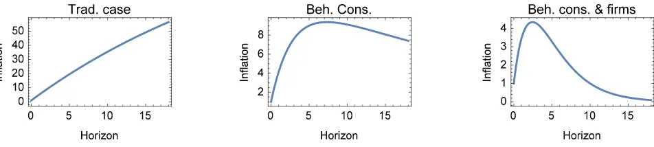
Suppose that the central bank announces at time 0 that it will cut the rate at time T, following a policy δt = 0 for t 6=T, δT <0, where δ is the interest rate gap. What is the impact? This is the thought experiment analyzed by McKay, Nakamura and Steinsson (forth.) with rational agents, which I pursue here with behavioral agents.
Figure 1 illustrates the effect. In the left panel, the whole economy is rational. In the middle panel, consumers are behavioral but firms are rational, while in the right panel both consumers and firms are behavioral. We see that indeed, announcements about very distant policy changes have vanishingly small effects with behavioral agents – but they have the biggest effect with rational agents. We also see how the bounded rationality of both firms and consumers is useful for the effect.
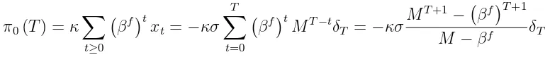
Formally, we have xt =M xt+1 −σδt, so xt =−σMT−tδT for t ≤T and xt = 0 for t > T. This implies that inflation is:
π0(T) =κ
X
t≥0
βftx
t=−κσ T
X
t=0
βftMT−tδ
T =−κσ
MT+1− βfT+1
M −βf δT
My take is that this issue is interesting (as are rational bubbles in general), but that the largest practical problem is to eliminate bounded equilibria. The behavioral model does that well.
Figure 1: This Figure shows the response of current inflation to forward guidance about interest rate in T periods, compared to a immediate rate change of the same magnitude. Units are yearly. Left panel: traditional New Keynesian model. Middle panel: model with behavioral consumers and rational firms. Right panel: model with behavioral consumers and firms. Parameters are the same in both models, except that (annualized) attention isM =Mf =e−ξ = 0.7 in the behavioral model, and M = 1 in the traditional model.
where βf := βMf is the discount factor adjusted for firms’ inattention. A rate cut in the very distant future has a powerful impact on today’s inflation (limT→∞π0(T) = 1−κσ−βf) in the rational
model (M = 1), and no impact at all in the behavioral model (limT→∞π0(T) = 0 if M <1).
When attention is endogenous, the analysis could become more subtle. Indeed, if other agents are more attentive to the forward Fed announcement, their impact will be bigger, and a consumer will want to be more attentive to it. This positive complementarity in attention could create multiple equilibria in effective attention M, mr. I do not pursue that here.
3.3
The ZLB is Less Costly with Behavioral Agents
What happens when economies are at the ZLB? The rational model makes very stark predictions, which the behavioral model overturns.
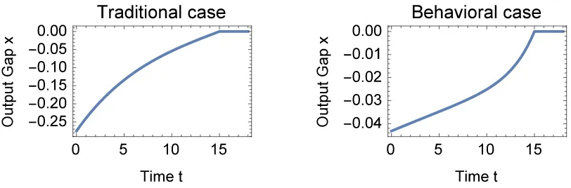
To see this, I follow the thought experiment in Werning (2012) (building on Eggertsson and Woodford (2003)), but with behavioral agents. I take rn
t =r for t≤T, and rnt =r for t > T, with
r < 0< r. I assume that for t > T, the central bank implements xt=πt= 0 by setting it = ¯r. At time t < T, I suppose that the CB is at the ZLB, so that it= 0.
Proposition 3.2 In the traditional rational case (ξ = 0), we obtain an unboundedly intense reces-sion as the length of the ZLB increases: limt→−∞xt =−∞. This also holds when myopia is mild,
ρξ σκ ≤1.
Figure 2: This Figure shows the output gap xt. The economy is at the Zero Lower Bound during times 0 to T = 15 years. The left panel is the traditional New Keynesian model, the right panel the behavioral model. Parameters are the same in both models, except that (annualized) attention is M =e−ξ= 0.7 in the behavioral model, and M = 1 in the traditional model.
We see how impactful myopia can be. We see that myopia has to be stronger when agents are highly sensitive to the interest rate (high σ) and price flexibility is high (high κ). High price flexibility makes the system very reactive, and a high myopia is useful to counterbalance that.
Figure 2 shows the dynamics. The left panel shows the traditional model, the right one the behavioral model. The parameters are the same in both models, except that attention is lower (set to an annualized rate of M = e−ξ = 0.7) in the behavioral model (against its value M = 1 in the traditional model).35 In the left panel, we see how costly the ZLB is (mathematically it
is unboundedly costly as it becomes more long-lasting), while in the right panel we see a finite, though prolonged cost. Reality looks more like the prediction of the behavioral model (right panel) – something like Japan since the 1990s – rather than the prediction of the rational model (left panel) – which is something like Japan in 1945-46 or Rwanda.
I note that this quite radical change of behavior is likely to hold in other contexts. For instance, in those studied by Kocherlakota (2016) where the very long run matters a great deal, it is likely that a modicum of bounded rationality would change the behavior of the economy considerably. Indeed, consider criterion (31).
4
Optimal Monetary and Fiscal Policy
4.1
Welfare with Behavioral Agents and the Central Bank’s Objective
Welfare is the expected utility of the representative agent, Wf = E0P∞t=0βtu(ct, Nt). This is the traditional welfare measure taken over the objective expectations. This is in accordance to the typical practice in behavioral economics, which views behavioral agents as using heuristics, but have experience utility from consumption and leisure like rational agents. 36 Following again the
literature, I do a Taylor expansion, so that fW = W∗+W, where W∗ is first best welfare, and W is the deviation from the first best. The next lemma calculates it
Lemma 4.1 (Welfare) The welfare loss from inflation and output gap is
W =−KE0
∞
X
t=0
1 2β
t π2
t +ϑx2t
+W− (34)
where
ϑ= κ
mfε (35)
K =ucc(γ+φ)κǫmf, and W− is a constant (explicited in (76)), and mf ∈(0,1]is firms’ attention
to the macro determinants of the markup, κ is Phillips curve coefficient, and ε is the elasticity of
demand. In particular, controlling for the value of κ, the relative weight on the output gap (ϑ) is
higher when firms are more behavioral (when mfis lower).
The traditional model gives a very small relative weightϑon the output gap when it is calibrated – this is often considered a puzzle. Here we obtain a larger weight – this is, a weight that is larger, conditional on a measure of ϑ. When firms react less to changes in inflation when setting their prices (when mf is lower), transitory inflation is less important for price setting, hence it is less distortive for allocation and welfare: so, inflation receives a lower weight in the objective function (so the relative weight on output (ϑ) is higher).
36In particular I use the objective (not subjective) expectations. Also, I do not count thinking costs in the welfare.
4.2
Optimal policy: Response to Changes in the Natural Interest Rate
4.2.1 When the ZLB doesn’t bind: Monetary policy attains the first best
Suppose that there is a productivity or discount factor shocks (they are not explicitly in the basic model, but can be introduced straightforwardly). This changes the natural real interest rate, rn
t.37 With rational and behavioral agents, the optimal policy is still to set it =rtn, i.e. to make the nominal rate track the natural real rate.38 This is consistent with x
t = πt = 0 at all dates. We obtain the first best. 39, 40
This is the traditional, optimistic message in monetary policy. However, when the natural rate becomes negative (and with low inflation), the optimal nominal interest rate is negative, which is by and large not possible.41 That is the ZLB. Then, much research has shown that the policy is
quite complex then. However, I now show how the policy becomes (in theory) easy and simple with rational agents.
4.2.2 When the ZLB binds: “Helicopter drops of money” as an optimal cure in the
Optimal Mix of Fiscal and Monetary Policy
Now I explore how behavioral agent change a lot policy at the ZLB, and indeed use the model’s ability to have non-trivial monetary and fiscal policy. By “fiscal policy” I mean transfers (from the government to the agents), and “helicopter drops of money”, i.e. checks that the central bank might send (this gives some fiscal authority to the central bank).42
To make the point, I suppose that we have a “crisis period” I = (T1, T2), with rnt < 0 during that period, so that the ZLB binds. But rn
t > 0 outside that period. With monetary policy only, the situation is dire, and we lose the first best.43 However, with fiscal policy and behavioral agents,
37Behavioral biases modulate the way TFP shocks change the natural interest rate, as for instance they affect the
effective intertemporal elasticity of substitution (see Section 8.2).
38If the inflation target was ¯π,the nominal rate would be real rate plus inflation targeti
t=rnt + ¯π. Throughout I assume ¯π= 0 for simplicity.
39As is well understood, to ensure equilibrium determinacy, the central bank imbeds this in-sample policy into a
more general rule, e.g. sets it=rtn+φππt+φxxt with coefficients φπ, φx suffiently large (following (30). On the equilibrium path, πt=xt= 0, so that it=rnt.
40If there are budget deficits, the central bank must “lean against behavioral biases”. For instance, suppose that
(for some reason) the government is sending cash transfers to the agents, dt>0. That creates a boom. Then, the optimal policy is to still enforce zero inflation and ouput gap (in the IS curve (23)) by setting: it=rtn+bσddt.
41Recent events have seen nominal rates slightly below 0%, but it does not seem possible to obtain very low nominal
rates, say -5%, for long, because stockpiling cash in a vault is then a viable alternative.
42The central bank could also rebate the “seignorage check” to the taxpayers rather than the government, and
write bigger checks at the ZLB, and smaller checks outside the ZLB.
43The first best is not achievable, as been analyzed by a large number of authors, e.g. Eggertson and Woodford
the first best can be restored.
Proposition 4.2 (Optimal mix of fiscal and monetary policy in a ZLB environment). The following monetary and fiscal policies yield the first best (xt = πt = 0) at all dates. During the crisis
(t∈(T1, T2)), use fiscal policy
dt=−
σrn t
bd
,
i.e. run a deficit with low interest rates, it= 0. After the crisis (t≥T2), pay back the accumulated
debt by running a government fiscal surplus and keeping the economy afloat with low rates, e.g.
dt= R−1(BT2 −B0) (1−ρd)ρ
t−T2
d <0 for some ρd ∈(0,1), and adjust it = bdσdt <0 to ensure full
macro stabilization, xt =πt= 0. Before the crisis (t < T1), there is no preventive action to do, so
set it=dt= 0.
Proof. The proof is simply by examination of the basic equations of the NK model, (23)-(24). We adjust the instruments so that xt =πt = 0 at all dates. Note that there are multiple ways to soak up the debt after the crisis, so that dt=R−1(BT2 −B0) (1−ρd)ρ
t−T2
d is simply indicative.
The ex-ante preventive benefits of potential ex-post fiscal policy. Proposition 4.2 shows that “the possibility of fiscal policy as ex-post cure produces ex-ante benefits”. Imagine that fiscal policy is not available. Then, the economy is depressed at the ZLB during (T1, T2). However,
it is also depressed before: because the IS curve is forward looking, output threatens to be depressed before T1, and that can put the economy to the ZLB at a time T0 beforeT1. Hence, the threat of a
ZLB-depression in (T1, T2) creates an earlier recession at (T0, T2) with T0 < T1. Intuitively, agents
feel “if something happens, monetary policy will be impotent, so large dangers loom”. However, if the government has fiscal policy in its arsenal, the agents feel “worse case, the government will use fiscal policy, so there is no real threat”, and there is no recession in (T0, T1). Hence, there is a
possibility of fiscal policy as an ex-post cure to produce ex-ante benefits.
In general, monetary and fiscal policies are substitutes (dt and it enter symmetrically in (23)), so a great number of policies achieve the first best. However, fiscal policy dt helps monetary policy if there is a constraint (e.g. at the ZLB), so the possibility of future fiscal policy is a complement to the monetary policy (as it relieves the ZLB).44
44This “second instrument” could be very useful even in normal times, in a richer model with capital. Suppose
4.3
Optimal Policy with Complex Tradeoffs: Reaction to a Cost-Push
Shock
The previous shocks (productivity and discount rate shocks) allowed monetary policy to attain the first best (without ZLB). I next consider a shocks that doesn’t allow the monetary policy to reach the first best, so that trade-offs can be examined. Following the tradition, I consider cost cost-push shock, i.e. a disturbance νt to the Phillips curve, which becomes:
πt=βMfEt[πt+1] +κxt+νt (36)
and the disturbance νt follows an AR(1), νt=ρννt−1+ενt. For instance, if firms’s optimal markup increases (perhaps because the elasticity of demand changes), they will want to increase prices and we obtain a positive νt (see Gali (2015, Section 5.2) for microfoundations).
What is the optimal policy then? Following the classic distinction, I examine the optimal policy first if the central bank can commit to a actions in the future (the “commitment” policy), and then if it cannot commit (the “discretionary” policy) and if it
4.3.1 Optimal commitment policy
The next proposition states the optimal policy with commitment. I normalize the initial (log) price level to be 0 (p−1 = 0).
Proposition 4.3 (Optimal policy with commitment: suboptimality of price-level targeting) The optimal commitment policy entails:
πt =
−ϑ
κ xt−M
fx t−1
(37)
so that the (log) price level (pt=Ptτ=0πτ) satisfies
pt =
−ϑ
κ xt+ 1−M
f t−1
X
τ=0
xτ
!
(38)
With rational firms (Mf = 1), the optimal policy involves “price level targeting”: it ensures that the
price level mean-reverts to a fixed target (pt = ϑκxt→0 in the long run). However, with behavioral
firms, the price level goes up (even in the long run) after a positive cost-push shock: the optimal
0 5 10 15 20
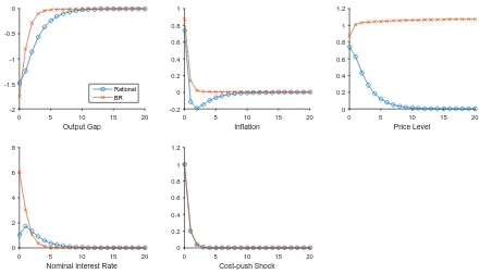
Figure 3: This figure shows optimal interest rate policy in response to a cost-push shock (νt), when the central bank follows the optimal commitment strategy. When firms are rational, the optimal strategy entails “price level targeting”, i.e. the central bank will engineer a deflation later to come back to the initial price level. This is not the optimum policy with behavioral firms. This illustrates Proposition 4.3.
“Price level targeting” and “nominal GDP targeting” are not optimal anymore when
firms are behavioral Price level targeting is optimal with rational firms, but not with behav-ioral firms. Qualitatively, the commitment to engineer a deflation later helps today, because firms are very forward looking (see Figure 3). That force is dampened in the behavioral model. The recommendation of price level targeting, one robust prediction of optimal policy model under the rational model, has been met with skepticism in the policy world– in part, perhaps, because its justification isn’t very intuitive.45 This lack of intuitive justification may be caused by that fact
that it’s not robust to behavioral deviations, as Proposition 4.3 shows.
Likewise, “nominal GDP targeting” is optimal in the traditional model, but it is suboptimal with behavioral agents.
45This is not a particularly intuitive fact, even in the rational model: technically, this is because the coefficientβin
0 5 10 15 20
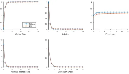
Figure 4: This figure shows optimal interest rate policy in response to a cost-push shock (νt), when the central bank follows the optimal discretionary strategy. The behavior is very close, as the central bank does not rely on future commitments for its optimal policy. This illustrates Proposition 4.4.
Other considerations Figure 3 gives some more intuition. Look at the behavioral of the interest rate. The policy response is milder with rational firms than with behavioral firms. The reason is that monetary policy (especially forward guidance) is more potent with rational firms (they discount the future at β,not at the lower rate βmf < β), so the central bank can act more mildly to obtain the same effect.
The gains from commitment are lower, as agents don’t react much to the future.
4.3.2 Optimal discretionary policy
Proposition 4.4 (Optimal discretionary policy) The optimal discretionary policy entails:
πt =
Let us first examine the comparative statics controlling for κ. For transitory shocks (ρν = 0), the optimal policy is independent of the firms’ bounded rationality. Future considerations don’t matter. However, for persistent shocks, the optimal policy is less aggressive (dit
dνt is lower) when
firms are more behavioral. This is because, with more myopic firms, future cost push shocks do not affect firms’ pricing today much, hence the central bank needs to respond less to them.46
5
Enriching the Model with Long-Run Changes to Inflation
5.1
Enriched Model
So far all variables came back to a steady state value normalized to 0. This is sufficient for most of the analysis. Here, I extend the analysis to allow for the possibility that long run inflation might change.47 For good measure, I also extend the model to have backward looking terms, which has
proven useful in empirical analyses, as this creates inertia in inflation (e.g. Gal´ı and Gertler 1999). The interaction of backward looking terms for firms and permanent changes will prove fruitful.
To handle this case, it is good to have a slight generalization of the model. A microfoundation presented in the appendix (Section 9.2) leads to the following model.
Proposition 5.1 (Behavioral New Keynesian model – three equation version) We obtain the fol-lowing behavioral version of the New Keynesian model, for the behavior of output gapxtand inflation
πt:
xt =MEt[xt+1] +bddt−σ(it−Etπt+1−rnt) (40)
πt =βfEt[πt+1] +απdt +κxt (41)
πtd+1 =πtd+γ ζπtCB + (1−ζ)πt−πdt
(42)
with α, βf :=βMf, γ, ζ are all in [0,1] and α+βf ≤ 1. The new term are πd
t, “default inflation”
coming from indexation, and πCB
t , the “inflation guidance” by the central bank.
46Things are more complicated when we don’t control forκ. Plugging the endogenous values ofκandMf (21-22) into (39), we see obtain:
it=
ϑ
(¯κmf)2+ϑ1−βm¯ hθ+ (1−θ) 1−βθ
1−βθm¯mf
i
ρν νt
Hence the optimal policy is again less aggressive when firms are more behavioral by decreasing m, but the effect of
mf is ambiguous.
48
In the microfoundation, each firm has two ways of predicting future inflation: one is via “purely rational expectations”, with πt, another is via default inflation, πd
t. I view this default inflation as a simpler, more available source of signal about future inflation.
Leading old and new Keynesian models are embedded in the structure (40)-(42), as we shall see.
5.2
Long Run Behavior and Determinacy
Given our system (40)-(42), we ask two questions: does Fisher neutrality (or something close to it) hold? Is the economy stable? The analysis will reveal a connection between those properties.
We first make a few observations. Consider the long run value of inflation (π∞) and the nominal rate (i∞). Their link is as follows.
Proposition 5.2 (Long run Fisher neutrality)If long run inflation is higher by dπ∞, then the long
run nominal rate is higher by di∞, where:
di∞
dπ∞
= 1− 1−α−β
f(1−M)
κσ (43)
Proof. Simply plug constant values of πt = πtd = πCBt = π∞, and xt = x∞ into (40)-(42). Then, we find i∞
π∞ = 1−
(1−α−βf)(1−M)
κσ . In addition, x∞=
−i∞(1−α−βf)σ
κσ−(1−α−βf)(1−M).
Next, I ask: is the equilibrium determinate? Is it stable?49
The next Proposition generalizes the earlier criterion (Proposition 3.1) to the case with backward looking terms.
Proposition 5.3 (Equilibrium determinacy with behavioral agents – with backward looking terms)
The system is stable only if:
φπ +
αζ+ 1−α−βf(1−M +σφx)
κσ >1. (44)
48Gali and Gertler (1999) present a model with partially backward looking firms: their model has γ = 1, ζ = 0,
M = 1. However, they haveζ= 0, which prevents the stability analysis below, whereζ >0 is crucial.
49Technically, this is the following. Define z
t := xt, πt, πtd
, taking πCB
t as given, and write the system as
Now, which properties of real economies should a model reflect? First, in the long run, a steady state rise of in the nominal rate is associated with a rise in inflation: di∞
dπ∞ >0, something we might
call “long run Fisher sign neutrality” (pure Fisher neutrality would be di∞
dπ∞ = 1). Most studies (e.g.
Kandel, Ofer and Sarig 1996, Evans 1998) find di∞
dπ∞ > 0 – though typically also they reject pure
Fisher neutrality (di∞
dπ∞ = 1), and instead find
di∞
dπ∞ <1, qualitatively as in Proposition 5.2.
50 This
means, given (43), that the data wants:
1−α−βf(1−M)
κσ <1. (45)
Second, in the recent experience in Japan (since the late 1980s) and in Europe and US (since 2010), the interest rate has been stuck at the ZLB, but without strong vagaries of inflation or output. Hence, following Cochrane (2015), I hypothesize that another desirable empirical “target” for the model is that the economy is stable even if the monetary policy is stuck at the ZLB forever.51
In the model, that means that (use (44) in the case φπ =φx = 0):
αζ+ 1−α−βf(1−M)
κσ >1. (46)
The next proposition records the tension between those two desirable properties, and a resolu-tion.
Proposition 5.4 (Long run links between inflation, nominal rates and stability)We have a positive long run link between inflation and nominal rates (45) and economic stability under passive monetary
policy (46) if and only if αζ is large enough and agents are boundedly rational (M <1), and prices are sticky enough (and as before, if prices are sticky enough). Ifαζ = 0(and “central bank guidance” has no impact) or M = 1, the two criteria cannot be simultaneously fulfilled.
This proposition means that the system is determinate if enough agents follow the central bank’s “inflation guidance”, πCB
t (i.e. if αζ is large enough). Intuitively, then, agents are “anchored” enough and the system has fewer multiple equilibria. Bounded rationality makes people’s decision less responsive to the future (and in the old Keynesian model, to the past). As a result, it reduces the degree of complementarities, and we can more easily have only one equilibrium (this is quite a 50The identification problems are very difficult, in part because we deal with fairly long run outcomes on which
there are few observations.
51This is a controversial issue, as other authors have argued that the instability of the 1970s in the US was due to
general point).
Leading old and new Keynesian models violate criterion (46), and allow for an unstable economy at the ZLB
The Old Keynesian model of Taylor (1999) has:52 ζ =βf = 0, α= 1. As a result, criterion (46) is violated if monetary policy is passive (as it is at the ZLB). However, criterion (46) tells us how to get stability in an Old Keynesian model: have ζ >0. If the economy is at the ZLB, we avoid the deflationary spiral because of bounded rationality. We need M < 1, and also αζ > 0, i.e. current inflation is not very responsive to its past and future values.53
The traditional New Keynesian model has M = 1, so there is no stability (criterion (46) is violated). With M < 1, we can get stability. But to get “Fisher sign neutrality”, π∞/i∞ >0, we need αζ >0.
Hence, I conclude that the enrichment of this model is useful for both Old Keynesian and New Keynesian models.
Speculating somewhat more, this usefulness of “inflation guidance” may explain why central bankers these days do not wish to deviate from an inflation target of 2% (and go to a higher target, say 4%, which would leave more room to avoid the ZLB). They fear that “inflation expectations will become unanchored,” i.e. that ζ will be lower: agents will believe the central bank less, which in turn can destabilize the economy.
5.3
Impulse Responses
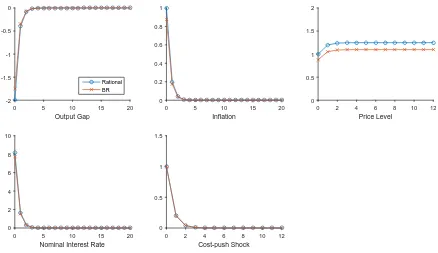
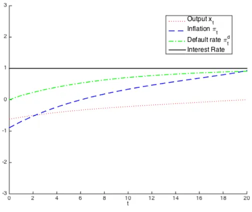
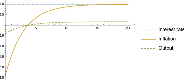
A permanent shock to inflation. To study this system, I assume a permanent rise of 1% in the nominal rate, with πCB
t = 1%. Figure 5 shows the result.54 On impact, there is a recession: output and inflation are below trend. However, over time the default rate increases: as the central bank gives “guidance” πCB
t >0, inflation expectations are raised. In the long run, for this calibration, we obtain Fisher neutrality.
This effect is very hard to obtain in a conventional New Keynesian model. Cochrane (2015) documents this, and explores many variants: they all give that a rise in the interest rate creates a rise in inflation (though Cochrane needs to select one particular equilibrium, as the traditional model generates a continuum of bounded equilibria). However, here the bounded rationality of
52It also replacesi
t−Etπt+1byit−πt, and there is axt−1term in the IS equation, but that is a fairly immaterial
difference.
53The Taylor model does feature a deflationary spiral, because it hasζ= 0.
Figure 5: Impact of a permanent rise in the nominal interest rate. At time 0, the nominal interest rate is permanently increased by 1%. The Figure traces the impact on inflation and output. Units are percents.
agents overturns this result, with just one bounded equilibrium.
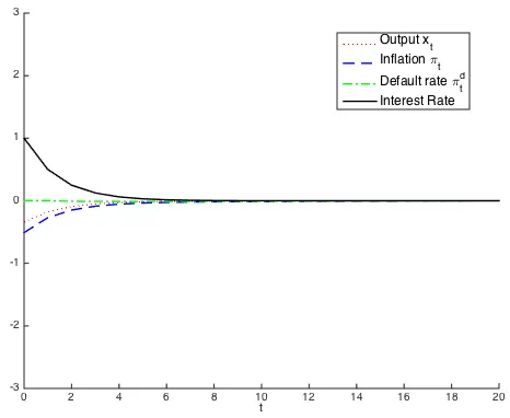
A temporary shock to the interest rate. I now study a temporary shock to the interest rate, it = i0e−φt for t ≥ 0. As the long run is not modified, I assume an inflation guidance of 0,
πCB t = 0.
Figure 6 shows the result. On impact, inflation and output fall, and then mean-revert. The behavior is very close to what happens without the backward looking term, i.e. setting α= 0.
For most purposes, I recommend the basic model of Proposition 2.6. However, when the long run changes, the extension proposed in this section is useful. Substantively, it yields the insight that the economy is stable if agents are boundedly rational (M < 1) and they follow enough the “inflation guidance” by the government. Also, for empirical purposes, the extra backward term is helpful (Gali and Gerler 1999).
6
Conclusion
This paper gives a simple way to think about the impact of bounded rationality on monetary and fiscal policy.
microe-Figure 6: Impact of a temporary rise in the nominal interest rate. At time 0, the nominal interest rate is temporarily increased by 1%. The Figure traces the impact on inflation and output. Units are percents.
conomic contexts `a la Arrow-Debreu (Gabaix 2014) and on dynamic settings with general dynamic programming (Gabaix 2016). Those microfoundations not only should give the model user good conscience, but they ensure for instance that model parameters respond to incentives in a sensible way, and that the model generalizes.
Furthermore, we have seen that the model has good empirical support for its main non-standard elements. For instance, when Gal´ı and Gertler (1999) estimate a Phillips curve, they estimate a coefficient on inflation ofβMf ≃0.75 at the annual frequency, which leads to an attention parameter of Mf ≃ 0.8 (at the annual frequency). In the IS curve, the literature on the forward guidance puzzle, using a mix of market data and thought experiments, gives good evidence that we need
M < 1, a main contention of the model. Finally, the notion that a higher interest rate lowers inflation in the short run (Keynesian effect), then raises it in the long run (classical Fisherian effect) is generally well accepted, using again a mix of historical episodes and empirical evidence. This is generated by the model, and is hard to generate by other models (Cochrane 2015).
In conclusion, we have a model with quite systematic microfoundations and empirical support for its non-standard features, that is also simple to use.
This paper leads to a large number of natural questions.