Money in a New Keynesian model estimated

(1)

Money in a New-Keynesian model estimated

with German data

Jana Kremer

Giovanni Lombardo

Thomas Werner

Discussion paper

(2)

Editorial Board: Heinz Herrmann Thilo Liebig

Karl-Heinz Tödter

Deutsche Bundesbank, Wilhelm-Epstein-Strasse 14, 60431 Frankfurt am Main,

P.O.B. 10 06 02, 60006 Frankfurt am Main

Tel +49 69 9566-1

Telex within Germany 41227, telex from abroad 414431, fax +49 69 5601071

Please address all orders in writing to: Deutsche Bundesbank,

Press and Public Relations Division, at the above address or via fax No. +49 69 9566-3077

Reproduction permitted only if source is stated.

(3)

Abstract

In this paper we estimate a simple New-Keynesian DSGE model with German data for the sample period 1970:q1 to 1998:q4. Contrary to a number of recent similar papers estimated with US and euro-area data, we find that real money balances contribute significantly to the determination of inflation and of the dynamics of output. We estimate our model using a maximum likelihood technique under a full set of structural shocks. We do not rule out indeterminate solutions a priori. Under multiple stable paths we close the model using the minimum-state-variable solution.

Keywords: Maximum-Likelihood, DSGE, MSV solution, New-Keynesian model, Germany.

(4)

Zusammenfassung

In diesem Diskussionspapier sch¨atzen wir ein einfaches Neukeynesianisches

dynami-sches Gleichgewichtsmodel f¨ur deutsche Daten und den Zeitraum zwischen dem

er-sten Quartal 1970 und dem letzten Quartal 1998. Im Unterschied zu einer Reihe

von anderen Arbeiten f¨ur die Vereinigten Staten von Amerika und dem Euroraum

(5)

List of Figures

1 The log-likelihood function and the MSV solution. . . 26

2 Response of the economy to a policy shock. . . 37

3 Response of the economy to a preference shock. . . 37

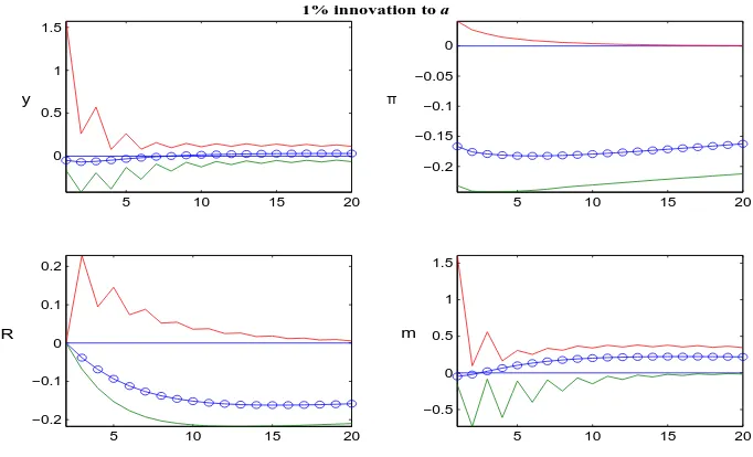
4 Response of the economy to a productivity shock. . . 38

5 Response of the economy to a money demand shock. . . 38

6 Response of the economy to a policy shock: ω = 0.65, γ2 = 1. . . 39

7 Response of the economy to a preference shock: ω= 0.65, γ2 = 1. . . 39

8 Response of the economy to a productivity shock: ω= 0.65, γ2 = 1. . 40

9 Response of the economy to a money demand shock: ω= 0.65, γ2 = 1. 40 10 Detrended per capita output and real balances. . . 41

11 Three-months nominal interest rate and quarterly inflation. . . 41

12 Actual and forecast values: a five year forecast horizon. . . 43

List of Tables

1 Calibrated parameters . . . 29

2 ML estimates and t-values: Lagged vs. contemporaneous policy feed-backs. . . 29

3 ML estimates and t-values . . . 30

4 ML estimates and t-values . . . 31

5 ML estimates and t-values: Whole sample with i.i.d. measurement errors. . . 32

6 Variance decomposition: Whole sample. . . 33

7 Variance decomposition: 1970:q1-1989:q4. . . 34

8 Variance decomposition: the 1970s. . . 35

9 Variance decomposition: the 1980s. . . 36

10 Fit of the model in comparison to a VAR. . . 42

(7)

Money in a New-Keynesian model

estimated with German data

∗

1 Introduction

In this paper we study the role of real balances in a stochastic general equilibrium model applied to German data. A number of recent papers have come to the con-clusion that real money balances play no statistically significant role in estimated New-Keynesian models. This is, for example, the evidence provided by Peter Ire-land (2002) for the USA and by Andr´es et al. (2001) for the euro area. The main motivation of our paper is to check the robustness of those findings to the German experience as interpreted by the same simple New-Keynesian model used by those authors.2

Our results suggest that real balances did indeed play an active role in Germany in the period 1970:q1-1998:q4.

Our model closely follows the work of Ireland (2002). In particular, we resort to the same simple New-Keynesian model, in which non-separable preferences are allowed between consumption and real balances. Non-separable preferences imply richer dynamics for output and inflation. Since the marginal utility of consumption is affected by the amount of real balances held by consumers, the intertemporal allocation of consumption is linked to the intertemporal allocation of real balances. This, in turn, affects the marginal propensity to supply labour and, hence, the real marginal cost of production. Under price rigidities (`a la Calvo (1983) and Rotemberg (1982)) the real balances enter the Phillips curve through the marginal cost. Under non-separability of preferences it is therefore impossible to solve the model without referring to the evolution of the real stock of money.

Once we allow for an active role of real balances, it is conceivable that the central bank – in our case the Bundesbank – will adjust its instrument (the nominal short run interest rate) in response to the developments in the market for money, inter alia. Therefore, our model displays an interest rate rule that links the quarterly interest rate to the rate of inflation, the output gap and the growth rate of money

∗_{This paper represents the authors’ personal opinions and does not necessarily reflect the views}

of the Deutsche Bundesbank.

2

(8)

balances. Our estimation shows that the Bundesbank responded significantly to all these variables.

By computing the variance decomposition for the endogenous variables of our model (output, inflation, the interest rate and real money balances) with respect to the exogenous shocks that the model incorporates (a technology shock, unexpected deviations from the policy rule called ‘policy shock’, a shock to the elasticity of substitution between consumption and real balances called ‘money demand shock’ and a shock to the intertemporal elasticity of substitution called ‘preference shock’), we are able to indicate the most likely sources of volatility of the German economy from the 1970s to the introduction of the euro. The relative weight of the four shocks in the determination of the volatility of our four variables seems to have changed over time, at least to some extent. Nevertheless, in comparison to the 1990s, the 1970s and the 1980s seem to be rather more homogeneous. Overall, it is hard to single out one specific shock as the main source of the total volatility of the economy. The estimation of dynamic stochastic general equilibrium models (DSGE) pre-sents some serious difficulties. First of all, these models, even in their simplest representation, involve a large number of parameters relative to the number of vari-ables. In order to increase the accuracy of the estimation it is therefore customary to calibrate some parameters at values taken from other empirical works. In this paper we follow this route, too, and we tend to do this in ways comparable with the work of Ireland (2002).

(9)

stable solutions. In this paper we adopt a different solution technique. Following the work by McCallum on the minimum state variable solution (MSV) we allow for only one particular type of solution under multiple stable paths (McCallum, 1999, 2002, 2003). Consistently with the MSV solution technique we always pick a state-space representation with a state-dimension invariant to the number of sta-ble roots.3

While this solution is of ‘point-size’ in the set of admissible solutions under indeterminacy, it permits the construction of a smoother likelihood function, besides being seen by some authors as economically sensible (see McCallum (1999, 2002, 2003) and Evans and Honkapohja (2001)).

The rest of the paper is organized as follows. Section (2) describes the model and section (3) the data used in the estimation. Section (4) describes and discusses the estimation technique. Section (5) presents and discusses the results. Section (6) concludes.

2 The model

Our model is a variant of a simple New-Keynesian closed economy model (e.g. Woodford (2003) and Clarida et al. (1999)). That is to say, it is characterized by a continuum of identical forward-looking households and a continuum of monopo-listically competitive firms that adjust their prices infrequently. We depart from the ‘purist’ New-Keynesian model in that we allow for non-separable preferences in consumption and real balances and in that we allow for a positive fraction of ‘backward-looking’ price setters (as in Andr´es et al. (2001)). The policy-maker is represented by an interest rate rule in the spirit of Taylor (1993). The details of the model are presented in the following subsections.

Households

An infinite number of identical households (of unit-mass) have preferences over a bundle of differentiated goodsCt, over labour lt and over real balancesmt =Mt/Pt.

Preferences over consumption goods and real balances are assumed to be non-additively separable. The household period-utility function takes the form

U(Ct, mt, lt) = at[V (Ct, g(mt, et))−L(lt)]

3

(10)

where et is a money demand shock and where g(mt, et) = m_e_tt.

The household maximizes the expected discounted (at rateβ) infinite stream of

its utility subject to the following budget constraint

s.t. Bs+Ms+PsCs =Rs−1Bs−1+Ms−1+wsls+ Πs+Ts, s=t, t+ 1. . .

Bs is nominal bonds (in zero aggregate net supply), Ms is end-of-period money

balances, Ps is the price of the consumption basket Cs, ws is the nominal wage, Πs

is the share of monopoly profits accruing to the household from the ownership of the firms, Ts are ‘government’ transfers and Rs is the gross nominal market return

on assets.

The consumption basket C is the CES aggregator

Cs =

where θ is the elasticity of the demand with respect to the relative price. The price of this basket is

Ps=

To this aggregator corresponds an optimal homothetic demand for each item i, i.e.

cs,i=

The solution of the household’s intertemporal problem yields the first-order con-ditions4

In order to express the first-order conditions in log-linear form we note that

ˆ

(11)

where the subscript ss denotes steady-state values and ˆxt≡log(xt)−log(xss).

We also introduce the following notation, which makes use of the normalization

ess = 1:

We can then write (in log-deviations) the consumption Euler equation as

σEtCˆt+1 =

and the money demand equation as

ˆ

mt =γ1Cˆt−γ2Rˆt+γ3eˆt (7)

where ˆRt is the log of the gross nominal interest rate (or, to a first-order

approxi-mation, the nominal interest rate), ˆπt+1 ≡Pˆt+1−Pˆt is the inflation rate and

An infinite number of firms (of unit-mass) sell their imperfectly substitutable goods in monopolistically competitive markets. The technology used by the firms to pro-duce their goods is

yi,t =ztli,t =ztlt=yt

where zt is a stochastic productivity shock.

We assume that firms adjust prices only at random intervals, in accordance with the mechanism described in Calvo (1983). More precisely, in any period of time

there is a probability ξ that a given firm does not adjust the price and hence it

(12)

Gal´ı and Gertler (1999) and Gal´ı et al. (2001) have shown that the dynamics of inflation (in the USA and euro-area, respectively) can be better captured by a Phillips curve that contains both forward-looking and backward-looking inflation terms: the so called ‘hybrid’ New-Keynesian Phillips curve. Like Andr´es at al. (2001), we therefore estimate a hybrid New-Keynesian model. We assume that

among the firms that adjust their price, a fraction (1 −γf) sets the price in a

backward-looking fashion, namely

Pb

t =Pt−1πt−1

That is, the backward-looking firms merely update their latest price by the inflation

rate that prevailed during the previous quarter. The other γf firms choose the

optimal price by solving the following problem

max

where T C denotes the total costs of production.5 The solution to this problem yields

pi,t =

θ−1 is the mark-up. The market clearing condition is given by yt,i =ct,i.

The first-order approximation of the optimal price equation gives

ˆ

where (using the household’s first-order condition and the labour-market clearing condition) approximation, the price index Pt can be written as

ˆ

(13)

By subtracting ˆPt−1 on both sides of the last expression we obtain ˆ

pi,t−Pˆt =φ1πˆt−φ2πˆt−1 (12) where

φ1 =

1−(1−ξ)γf

(1−ξ)γf

(13)

φ2 =

1−γf

γf

(14)

Finally, replacing equation (12) into (9) yields the hybrid New-Keynesian Phillips curve

ˆ

πt=

1

φ1+ξβφ2

[(1−ξβ) ˆmct+Etξβ(1 +φ1)ˆπt+1+φ2πˆt−1] (15)

Monetary policy

Following Ireland (2002), we assume that the monetary policy followed by the Bun-desbank can be represented by a modified Taylor rule (Taylor, 1993). The short-run interest rate, in deviation from the steady-state value, is adjusted in response to inflation, the output deviation from trend and the growth rate of real balances.6 _We also allow for a white-noise policy shock. This can be best interpreted as quarterly deviations of the nominal interest rate from the policy rule. Furthermore, we allow for an auto-recursive component in the rule. This is typically found to improve the statistical fit of estimated policy rules (e.g. Clarida et al. (1998)). Woodford (2003) among others, argues that an inertial policy rule can result from the objective of the central bank. We do not explore the micro-foundations of the policy rule.

The results we report here are estimated with the interest rate rule

ˆ

Rt=ρRRˆt−1+λππˆt−1+λyyˆt−1+λµµˆt−1 + ˆνt (16)

where ˆµt= ˆmt−mˆt−1. We also estimated a version of the model where both lagged and contemporaneous variables appeared in the policy rule. The estimate ofωis only marginally affected by this amendment and is still significantly different from zero. The reaction coefficients on the lagged variables remain positive and significant.

6

(14)

The reaction to output is not significantly different from zero. Surprisingly, the response of the policy instrument to the contemporaneous inflation rate and to the contemporaneous growth rate real balances is significantly negative. On the basis of a likelihood-ratio test we should reject the null that the central bank reacted only to lagged variables (see Table (2)). Interestingly, the point estimates are consistent with a policy rule that would react negatively to an acceleration of the stock of money as well as to the quarterly growth rate of inflation. We find this result difficult to interpret economically. In particular the impulse responses produced by the larger model are not closer to our economic intuition than those produced by the model with a backward-looking policy. For these reasons, and given that the other parameters are not affected by the specifications of the policy rule, in the rest of the paper we discuss the results relative to the backward policy rule only.7

Exogenous disturbances

We assume that the exogenous stochastic forcing processes (in log deviation) can be described as follows

ˆ

at = ρaˆat−1+ǫa,t

ˆ

zt = ρzzˆt−1+ǫz,t

ˆ

νt = ǫR,t

ˆ

et = ρeeˆt−1+ǫe,t

where ǫi,t ∼N(0, σ2i) and E(ǫi,t+u, ǫj,t) = 0 for i6=j and for all u.

Reduced form of the model

The Euler equation (6), the money demand equation (7), the Phillips curve equation (15), the interest rate rule (16) and the four exogenous stochastic processes allow us to determine equilibrium values for output, inflation, the interest rate and the growth rate of the money stock. The reduced-form model in these four variables is estimated using the data series described in the following section.

7

(15)

3 Data

We use quarterly (seasonally adjusted) data for Germany from 1970:q1 to 1998:q4. In particular we use series for real GDP per capita, the change in the CPI index

as the measure of inflation,8 _{the three-months money market interest rate and the}

money aggregate M3 per capita. All series are taken from the Bundesbank’s data set.9

Since in the first years after the re-unification the East-German data for output and the CPI index show an abnormal behaviour, we use West-German data through 1992:q4. The post 1992 series for output, population and CPI index are constructed using the TRIAN technique. This amounts to deriving the 1993:q1 observation from the (West-Germany) 1992:q4 observation updated by the growth rate of the corresponding series for the re-unified Germany from 1992:q4 to 1993:q1. From there onwards the series is constructed recursively using the growth rate of the series relative to the re-unified Germany. For M3 we use a TRIAN-series constructed by the Bundesbank. The series for per capita output and per capita real money balances are detrended using the HP filter.

Figures (10) and (11) show the time series used in the estimation. Detrended output seems to capture the main business cycle episodes of the 1970s, 1980s and 1990s. As for inflation and the interest rate, the inflationary episodes of the early 1970s and early 1980s are noticeable.

It is also worth stressing that the Bundesbank officially announced a monetary targeting strategy only in December 1974 (Deutsche Bundesbank, 1995), although it also paid particular attention to the developments in the market for money prior to that. In the period between the starting date of our series and March 1973, the policy of the Bundesbank was constrained by the Bretton Woods agreements. Nevertheless, excluding the first three years from our data set did not alter our

8

The model does not distinguish between consumer prices and the GDP deflator. Moreover it is not clear which of the two indicators of inflation dominated the Bundesbank’s monetary policy decisions. Most likely, both indicators were taken into consideration. In earlier experiments we re-estimated the model using the GDP deflator instead of the CPI index. This left the results largely unchanged.

9

(16)

findings.

4 Estimation

Following Ireland (2002), we use a maximum-likelihood estimation of our model. The model has a ‘full set’ of structural shocks so that it can be taken directly to the data without resorting to measurement errors (e.g. Ireland (2003a), McGrattan et al. (1997)). The model, despite its simplicity, has a large number of parameters. Not all these parameters can be precisely estimated. Therefore we set some of them at ‘reasonable’ values. Among these calibrated parameters is the Calvo-probability of price adjustment (1−ξ). When we tried to estimate this parameter, the estimation

algorithm produces values close to the lower bound (ξ → 1), which is clearly not

admissible.10 _{Nevertheless, we believe that prices in Germany, in our sample period,} were probably less flexible than in the USA, as some evidence in the literature seems to suggest (e.g. Gal´ı et al. (2001), Hoffmann et al. (2003)). Hence we set ξ = 0.80, which amounts to the assumption that forward-looking firms typically adjust their prices after five quarters. It is similarly difficult to pin down a reasonable value for the Frish elasticity of labour supply ((ζ −1)−1

). We follow Ireland (2002) and set

ζ = 1. Earlier experiments showed us that the estimated degree of risk aversion in

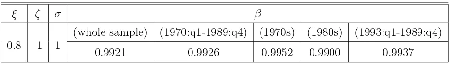
consumption (σ) is not significantly different from one. Since there are already a high number of estimated parameters, we set σ = 1 for the results reported here.11 The discount rateβ is set equal to the ratio of the sample mean of inflation and the gross nominal interest rate. Table (1) shows the calibrated parameters.

As in Ireland (2002) and Andr´es et al. (2001), the money demand equation requires an estimate for γ2 only, since the times series means together with σ, ω and γ2 give sufficient information to recover the values of the other money demand parameters. The estimated parameters are summarized in the following vector

Θ = [ρR, λy, λπ, λµ, ρa, ρz, ρe, σa, σz, σe, σR, ω, γ2, γf]

10

Christiano et al. (2001) argue that the precision of the estimates of the degree of nominal rigidity is very sensitive to the assumptions regarding the ‘real side’ of the economy. It is therefore not surprising that the Calvo probability cannot be easily estimated.

11

(17)

The state-space form of the model and its solution

The model can be written as

AEtwt+1 =Bwt+Cut

andA,B andCare matrices of coefficients. The structure of these matrices can eas-ily be induced from the structural equations of the model presented in the previous section.

The model is solved using the method discussed in Klein (2000). In this way the model is cast in a state-space form and – based on this form – the Kalman filter and, hence, the loglikelihood function is constructed. Numerical algorithms are then used to search for the vector of parameters Θ that maximizes the likelihood function. The likelihood function in terms of Θ usually has several local maxima, therefore convergence to the global maximum is a daunting task for any algorithm. We use a combination of three algorithms for this purpose: namely two ‘gradient-based’ methods12 _{and the ‘Simulated Annealing’ algorithm (see Goffe et al. (1994)).}

Linear rational expectation (LRE) models are ‘vulnerable’ to indeterminacy, or multiple stable solutions. This is, for example, the case when the ‘Taylor principle’ does not hold (Woodford, 2003). When the response of the central bank to changes in inflation is not sufficiently aggressive, the real interest rate does not move in the correct direction, so that in principle any ‘prophecy’ of inflation is self-fulfilling. In this event there are potentially infinite ways in which the model can be closed.13 This fact constitutes a major problem in estimating LRE general equilibrium mod-els. Most of the research in this area imposes a rather strict assumption on the model by ruling out indeterminate solutions. The likelihood function is then max-imized under the constraint that the parameter vector Θ does not yield multiple

12

One is the built-in fminunc.m code in MATLAB, while the other is a more sophisticated (and robust) algorithm (SolvOpt) written by Kuntsevich and Kappel (1997).

13

(18)

stable solutions: for example, by imposing the constraint that the policy parame-ters obey the Taylor principle. One problem that might arise from this assumption is that estimated standard deviations and confidence intervals might be invalid, since they might embrace combinations of parameter values that yield indeterminacy and that, therefore, were deemed improbable to start with. Furthermore, the numeric maximization of the likelihood function might be corrupted by the impossibility to ‘wander’ through the indeterminacy region even when the maximum is beyond that region: that is, it is more likely to end up in a local maximum. Finally, when the maximum is too close to the indeterminacy region, it can be impossible to compute the Hessian and hence the standard errors for the estimates.

In this paper we follow a different strategy. We assume that the elements of the state vector, in the solution of the LRE model, as well as the size of the transition matrix of the state-space form of the model are invariant to the number of stable roots of the system. This amounts to the MSV solution advocated by McCallum

in a number of papers (see McCallum 1999, 2002, 2003).14 _{In order to make the}

solution unique, McCallum uses a more restrictive definition of the MSV solution than that used here. We use the broader definition of an MSV solution given in Evans and Honkapohja (2001) and which allows for multiplicity. Furthermore, we take a pragmatic approach to the issue concerning the relevance of the MSV solution. By allowing for an MSV solution in the estimation of our model, we are less restrictive – although to a limited extent – than those that restrict the domain of the likelihood function to parameters that lie within the determinacy region. We let the likelihood function decide whether the MSV solution under multiplicity is better than any other combination of parameters that yields saddle-path stability. The Appendix describes more in detail how the MSV solution can be combined with the ML estimation of a LRE model.

5 Results

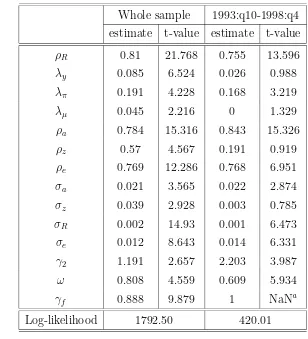
Tables (3) and (4) report the ML estimates (and t-values) of the parameters of our model for the period 1970:q1-1998:q4. We also consider the possibility that the

14

(19)

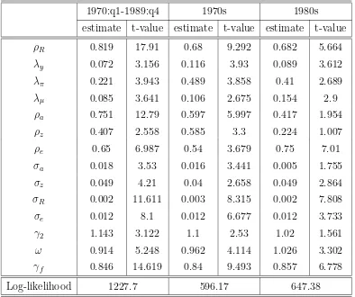
1970s the 1980s as well as the post-reunification period can be better described by different sets of parameters. This possibility is, for example, suggested by a casual look at the time series for output and money balances. In the 1970s the two series seem to have moved almost in step. A quite different picture emerges from the 1980s and 1990s. Therefore, Table (4) shows the estimates (t-statistics) relative to the pre-reunification period as well as relative to the 1970s and 1980s. The post reunification period is clearly more problematic for the quality of the data as well as for a clear transition of Germany (mainly East-Germany) to a new economic en-vironment. Table (3) shows the result based on the whole sample (1970:q1-1998:q4) alongside the results relative to the short sub-sample 1993:q1-1998:q4. Qualitatively and quantitatively the results are very similar whether we include the 90s or not. Indeed, unreported results show that similar estimates can be obtained by using

data on output and inflation relative West-Germany only.15

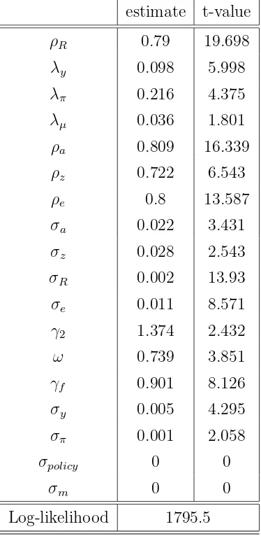
Our estimates seem not to be affected by the inclusion of i.i.d. measurement errors for the four time series at hand. Table (5) reports the point estimates and t-values of our model when four measurement errors are estimated simultaneously with the rest of the parameters. A notable difference between the point estimates obtained with measurement errors and those obtained in the restricted model is that technology is much more persistent in the former case than in the latter. While two of the four measurement errors are estimated to be significantly different from zero, the value of the log-likelihood function indicates that the null of no measurement errors cannot be rejected. Therefore, and for the sake of parsimony we focus our discussion on the model estimated without measurement errors.

An important difference between the ML estimates obtained for the whole sample and those obtained for the sub-sample 1970:q1-1989:q4 is that the former yields multiple stable equilibria, while the latter produce a unique saddle-path equilibrium. Nevertheless, the estimates for the whole sample seem to lie very close to the border of the indeterminacy region. Indeed it is easy to find a combination of parameters very similar to our ML estimates but that produces a saddle-path stable equilibrium. For example, by searching over the parameters that yield determinacy around the ML estimates we find

15

(20)

ρR λy λπ λµ ρa ρz ρe σa σz σR σe γ2 ω γf

0.813 0.084 0.189 0.051 0.778 0.546 0.762 0.02 0.041 0.002 0.013 1.264 0.796 0.874

The likelihood value for this set is 1792.4, i.e., compared to the value given in Table (3), the null of a saddle-path equilibrium cannot be rejected at any sensible s.l.. This set of parameters yields also the same dynamic response of the economy to the four shocks studied in this paper as the MSV-based estimates do. This result is not totaly obvious since, contrary to McCallum’s (2003) strict interpretation of the MSV solution, we do not impose a specific ordering of the stable eigenvalues.16 _In spite of this, the model displays a marked smoothness across the two regions.

As a central result, the estimates of the cross derivative of preferences over consumption and real balances (ω) are significantly different from zero.17

The order of magnitude of the point estimate is not very different from that found by Andr´es et al. (2001) for the euro area, although they find it not significantly different from zero. Our result stands instead in sharp contrast to the result of Peter Ireland (2002), who finds for the USA a point estimate virtually equal to zero and with a large standard error.

As for the policy rule, we find that the nominal interest rate is rather inertial and, apparently, more inertial than in the USA or in the euro area as a whole, although again this parameter is imprecisely estimated by Andr´es et al. (2001). The Bundesbank seems to have responded significantly to inflation and to our measure of output deviation from trend. Consistently with the Bundesbank’s monetary policy strategy up to the introduction of the euro, it also responded significantly to money growth (both as nominal and as real growth of M3). Notably, the response of the interest rate to M3 is very sensitive to the sample period. Including the post-reunification period yields an estimate for this coefficient that is half as large as that obtained for the pre-reunification period. Indeed, restricting the sample period to 1993:q1-1998:q4 yields a zero estimate for λµ (approximated to the third digit).

This result (although based on a rather small sample) could reflect a change of focus

16

McCallum’s ordering is intended to reduce the multiplicity of the MSV solutions. In most cases this ordering coincides with the set of smallest (in modulus) eigenvalues. Our point estimate does not conform to this criterion. Like McCallum, though, we keep constant the set of state variables made up of the exogenous shocks and predetermined variables that appear in the structural model.

17

(21)

of the Bundesbank in the face of the increased erratic behaviour of M3.18

The estimate of the share of forward-looking firms is significantly different from zero. The point estimate suggests that roughly 89% (85% in the pre-reunification period) of the firms set prices in a way that is consistent with forward-looking behaviour. This number is larger than that found by Andr´es et al. (2001) – i.e. about 61% – and by Gal´ı et al. (2001) – about 66%.

Compared to values typically used in calibrated models of this type, the model produces a relatively small estimate of the persistence of the technology shock. Preference and money demand shocks are significantly different from white-noise processes.

The estimates for the 1970s and 1980s are comparable to those for the whole sample. The most noticeable differences are related to the reaction coefficient on inflation in the policy rule (higher in the two sub-samples) and the parameters describing the preference shock (lower autocorrelation in the sub-samples). For the 1980s we obtain less precise estimates (smaller t-values).

These differences might certainly account for differences in the relative dynamic pattern of our variables. Another factor that may have affected the relative pattern of the observed series, independently or in conjunction with the change in param-eters, is the volatility of the underlying shocks. We will come back to this issue in discussing the variance decomposition of the endogenous variables with respect to the exogenous shocks (subsection 5.2).

5.1 Impulse responses

Figures (3) to (5) show the impulse responses for the four endogenous variables for

the full sample estimates. The graphs also show 95% confidence bands.19

The possibility of constructing confidence intervals around the impulse responses is one of the advantages of adopting an ML estimation technique, as opposed to sim-ple calibration. The Hessian of the log-likelihood function provides a measure of the

18

This does not necessarily imply that monetary aggregates became less important for the con-duct of monetary policy. Indeed the Bubdesbank as many other central banks spends relatively large resources in filtering and interpreting the information contained in the monetary aggregates. The 90s were a period in which monetary aggregates were particularly noisy.

19

(22)

statistical uncertainty related to our estimates. The simple plot of impulse responses based on the point estimate of Θ neglects that information about the accuracy of the estimates. So, for example, the estimated parameters of the preference shock are statistically different from zero while the impact response of output to an innovation to this shock is not (Figure (3)).

Let us now consider each of the shocks in turn. An unexpected increase in the interest rate (a policy shock) is described in Figure (2). It implies a persistent departure of the nominal interest rate, real balances and the inflation rate from their long-run equilibrium. A non-standard response of inflation is responsible for the dynamics of these variables which is related to the estimated complementarity of consumption and real balances: The higher interest rate leads via the money demand equation to lower real balances. The fall in the latter raises the marginal costs of production (see equation (10)) and, thus, the inflation rate (see (15)). Higher inflation and the interest rate inertia lead to an only slow adjustment of the interest rate and, through the described channel, also of real balances and inflation.

In particular, given the estimated parameters the model produces a ‘price-puzzle’ (e.g. Christiano et al. (2001)), even though the increase in inflation is not significant. Christiano et al. (2001) and Altig et al. (2003) obtain a negative impact-response of inflation to an expansionary monetary policy shock from an estimated VAR model. Furthermore, these authors provide a DSGE model that, through the assumption of ‘working capital’ can reproduce the positive co-movement between inflation and the interest rate. Under the ‘working capital’ assumption the interest rate enters the marginal cost directly while in our model the interest rate affects the marginal cost only indirectly through the marginal utility of consumption (and real balances). It should be noted, though, that the non-separability brings about the price-puzzle for sufficiently large values of ω only. For example, if we set ω to 0.65 and γ2 to 1, the price puzzle disappears (see Figure (6)).20

There is only a small impact of the policy shock on the real interest rate. Output

evolves in line with real money balances. Since ω is smaller than one and changes

in the real interest rate are only small the reaction of output is somewhat smaller (see equation(6)).

Turning to the conseqences of a preference shock, Figure (3) shows an impact

20

(23)

response of output that is difficult to reconcile with simple economic intuition: i.e. an increase in the intertemporal marginal rate of substitution of consumption should increase current consumption relative to future consumption. On the contrary, the point estimate implies the opposite result. The confidence bands suggests, though, that the effect of a preference shock on output is rather imprecisely estimated. At the 5% significance level we cannot reject the null hypothesis that output does not vary at all. On this respect, it is worth noting that the model estimated with measurement errors produces a positive response of output and money balances (result not shown). The rest of the impulse responses remain nevertheless virtually unchanged.

Figure (3) also shows that the real interest rate is positive for some quarters and returns nearly to its steady-state value thereafter.

The dynamics of the other variables following a preference shock can again be linked to the relation between inflation and money balances described by the esti-mated Phillips curve. The impact-response of inflation depends on the insignificant response of output. Thereafter the stronger increase in real balances relative to output has a negative effect on marginal costs (see equation (10)) and, hence, a dampening effect on inflation. Given the estimated policy rule, the fall of infla-tion and the inertia in the interest rate dominate the increase in real balances and output. Therefore, the interest rate remains persistently under the long-run equilib-rium. This is accompanied by a persistent deviation of real balances and inflation from their steady-state values.

The impulse responses were also derived under the assumption ω = 0.65 and

γ2 = 1 (see Figure (7)). Now ˆy moves up directly – in line with economic intuition.

This might indicate that the point estimate for ω is somewhat too high.

A more ‘standard’ story emerges from the analysis of a productivity shock (Figure (4)). Except for the first period, output and real balances significantly increase in the short run (up to about the sixth quarter). Inflation drops marginally (though significantly) in the first two quarters and then remains slightly above equilibrium for a long time. The top-left panel indicates that the central bank reacts to a technology shock with a persistent, although marginal, increase in the interest rate.

Under smaller values for ω and γ2 (as in Figure (8)) on impact a technology

(24)

then converges smoothly to the long run equilibrium.

Finally, an innovation to the money demand shock produces a significant fall in output followed by a persistent (and marginally significant) overshoot of the long-run equilibrium. Real balances, on the contrary, increase and remain (significantly) above the long-run equilibrium up until about the twelfth quarter. The nominal interest rate and inflation fall very slightly and the reaction is statistically insignif-icant. The alternative set of values for ω and γ2 considered in Figure (9) seem to change mainly the response of inflation and the interest rate.

An interesting feature of the money demand shock – shared only to a very limited extent by the policy shock – is that real balances and output tend to move in opposite directions in the very short run. By observing the time series of detrended output and real balances (Figure (10)), we note that there are periods (e.g. the 1970s) when both series seem to move in the same direction, while in others (e.g. the 1980s and the 1990s) they seem to move in opposite directions. It is tempting to think that the two periods have been dominated by different sets of shocks. The variance decomposition of the endogenous variables presented in the following section seems to point in the same direction.

5.2 Variance decomposition

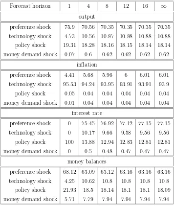
Table (6) shows the variance decomposition of our four endogenous variables with respect to the four shocks for the whole sample period. Compared with Table (7), relative to the sub-sample 1970:q1-1989:q4, it shows that the inclusion of the 90s dramatically changes the results. By including the post reunification period we obtain that most of the dynamics of output, interest rate and money balances is driven by preference shocks. Inflation is almost totally driven by technology shocks. Moreover, the forecasted output volatility can be attributed only minimally to money demand shocks. Given the poor quality of the post-reunification data we do not want to emphasize these results.

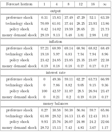
As for the pre-reunification period, Tables (7) to (9) suggest that there has been a shift in the balance of weights of the four shocks in accounting for the volatility of our four variables.

(25)

money demand shocks account for less than a quarter from the first year after the shock onwards. Preference shocks gradually increase their share in the total variance of output and become dominant only in the very long run. At business cycle frequency, it seems that the main source of German output volatility in the 1970s and 1980s was technology. Money demand shocks are relatively more important in the 1980s than in the 1970s. This latter fact seems to be consistent with the apparent change in correlation between real money balances and output documented in Figure (10).

The marked role for technology that emerges from the variance decomposition is consistent with the real business cycle (RBC) perspective. It has to be taken into account, though, that our model incorporates only one supply shock. Thus, part of the fluctuations of output that we attribute to technology shocks might actually come from a different type of supply shock. Ireland’s (2003b) work for the USA, for example, suggests that cost-push shocks – modelled as unexpected changes in the elasticity of demand for intermediate goods – played a role, too. Because both types of shocks move inflation and output in different directions, they could not be identified in the model as it stands. Therefore, Ireland (2003b) adds the unobservable variable ‘output gap’, defined as the deviation of output from its socially optimal level, to the policy rule. Since the technology shock but not the cost-push shock shifts the socially optimal level of output they can in principle be identified by their different influence on the (observable) nominal interest rate. In reality it is difficult, though, to estimate the past, let alone the contemporaneous output gap. It is therefore not obvious how the model’s output gap can be introduced into the policy rule.

Inflation in Germany’s 1970s and 1980s has been mainly driven by preference shocks (between about 46% and 70%). The second most important shock, the policy shock, never accounted for more than about 29% of total volatility, in relation to the whole sample. Policy shocks seem to have had a more important role in the 80s, where they accounted for about 42% of inflation volatility in the medium to long run. Also interestingly, in the very short run inflation in the 80s seem to have been driven mainly by technology shocks.

(26)

slightly tilted in ‘favour’ of the policy shock.

The forecast variance decomposition for the real money balances is markedly different across the two sub-periods. In the 1970s, preference shocks seem to have driven the volatility of real balances in the medium run. In the 1980s this role is more equally shared by the four shocks, although preference shocks play little role up to one year after the shock.

5.3 Empirical performance of the model

Finally, we discuss in this section the empirical performance of the DSGE model as compared with an unrestricted VAR estimated with the same data. The

log-likelihood values and the R2 _{values for the model, the VAR(1) and the VAR(4)}

are collected in Table (10). The log-likelihood of the VAR(1) (1814.4) is higher than the log-likelihood of the model (1792.5) and a formal test would reject the restrictions implicit in the model against the VAR(1). Nevertheless, it should be noted that although the VAR(1) is based on 20 estimated parameters and the model only on 10 structural parameters the total number of restrictions (linear and non-linear) is larger than 10.21 _{A comparison of the} _R2 _{values for the model with the} corresponding values for the VAR(1) shows that the DSGE model fits output and money fairly well. With respect to inflation and the interest rate the model fits the data only to a lesser degree. The fit of the VAR(1) can be beaten by a VAR(4), but only a the cost of a rather large number of estimated parameters.

It is important to mention, that using the in-sample properties of a model is not necessarily the best way to assess the empirical validity of a model. A model can perform very well in-sample but perform badly in an out-of-sample exercise. In such a case the model over-fits the data. An interesting exercise is therefore a comparison of the out-of-sample forecast properties of the model relative to a VAR. For this exercise we have used the estimated DSGE model, the VAR(1) and the VAR(4) for the 1970s and then forecasted the first five years of the 1980s. The actual and forecast values based on the model are shown in Figure (12). Clearly, the model can not forecast all fluctuations of the data, but it nevertheless captures the overall movement of money and output very well. In Table (11) some formal

21

(27)

measures of the forecast performance are summarized. Here RMSE is the Root Mean

Square Error and MAPE is the Mean Absolute Percentage Error.22 _{A lower value of}

these measures corresponds to smaller forecast errors. The DSGE model can beat the forecast performance of a VAR(1) for output and money. Both measures of the forecast errors are smaller for the model than for the VAR(1). Even a VAR(4) with a large number of estimated parameter (68) can not beat the DSGE model. For inflation and for the interest rate the DSGE model is clearly beaten by the VAR(1) and VAR(4).

Given the simplicity of our model, its ability to fit the data is remarkably good and comparable to the performance of unrestricted VAR models based on the same data set.

6 Conclusions

This paper has taken a simple New-Keynesian model with non-separable preferences in real balances and consumption to German data for the sample period 1970:q1 to 1998:q4. Following the recent related literature, we have used a maximum likelihood estimation under a full set of structural shocks. The main contribution of this paper is to show that the separability of preferences found for the USA by Peter Ireland (2002) and for the euro area by Andr´es et al. (2001) is not borne out by German data. We can reject the null hypothesis that real balances do not enter the Phillips curve and the IS (consumption Euler) equation. Real balances seem to have played an active role in the determination of the dynamics of output and inflation from the 1970s through the 1990s. Our estimated interest rate rule – i.e. the rule that should reflect the policy of the Bundesbank – is consistent with this role of the real balances. The Bundesbank seems to have adjusted its short-run interest rate in response to variations in the growth rate of money, as well as in response to inflation and output variations. We deem our findings important since it has become customary to refer to the evidence on the separability as a stylized fact. Our result suggests that there might be cross-country differences in the role played by the stock of money. This might have consequences for the conduct of monetary policy within a monetary union that does not display homogeneity in terms of the role of real balances in the

22

These measures are computed as RMSE = (1/HPH_t=1(yt − ft) 2

)1/2

and MAPE = 100/HPH_t=1|

yf−ft

yt |, with actual values of the data yt and forecasted values ft. The forecast

(28)

business cycle. This normative aspect deserves further investigation.

The impulse-response analysis based on our ML estimates suggest that the es-timated degree of complementarity between real money balances and consumption (together with the interest rate elasticity of money demand) is probably too large to produce economically sensible results. Nevertheless, we have shown that taking ac-count of the parameter uncertainty more sensible impulse responses can be obtained under non-separable preferences.

Our model has also indicated the most likely sources of volatility of the German economy in the 1970s, 1980s and 1990s, although the results relative to the latter period might by strongly affected by the poor quality of the available data. At least up to the 1990s, preference and policy shocks seem to have driven the volatility of inflation and the interest rate. Less easy is to single out the major determinant of the volatility of output and real money balances. Nevertheless, we have also pointed out that there are possibly other shocks that could account for the volatility of the German economy and which we have not explicitly considered in our model. We have argued that to some extent it would be difficult to disentangle these alternative shocks from the four shocks considered here, at least in the current version of our model.

The impulse-response analysis together with the decomposition of the forecast variance and the values of the point estimates, lead us to believe that relative to the 1970s the 1980s have witnessed more pronounced money demand shocks (relative to the other shocks).

From a methodological point of view, our paper contributes to the existing lit-erature in that we have combined the standard maximum-likelihood estimation of a DSGE model with the idea that multiple stable solutions, arising in LRE models for certain combinations of parameter values, can be modelled using the minimum state variable criterion advocated by McCallum (1999). Using this approach we have found that the ML estimate for the whole sample yields multiple stable solutions. Nevertheless we have also shown that the null of a determinate (saddle-path) equi-librium cannot be rejected at any sensible significance level. In the neighborhood of our point estimates the economy behaves in a way that is independent of the multiplicity of the stable solutions.

(29)

Appendix

A

ML estimation of a Linear Rational

Expecta-tion model using the MSV soluExpecta-tion

In this section we show how a LRE model can be estimated via ML after being solved with the MSV algorithm.

Let us write the LRE model as

AEt[xt+1] =Bxt+Cµt

µt=Rµt−1+ǫt (17)

ǫt ∼i.i.d(0,Σǫ)

where xt is a vector of endogenous variables andµt is a vector of exogenous forcing

processes. This dynamic problem can be written in its state-space form. For this purpose we note that xt = [st, ct]′, where st are ns predetermined variables and ct

are nc control variables. In order to write the stationary state-space form we need

to decompose the matrices A and B in their spectral form (i.e. their generalized

eigenvalue-eigenvector form) (e.g. Blanchard and Kahn (1980) or Klein (2000)). This decomposition is affected by the number of stable eigenvalues of the system.

Definition 1 Let λ be the (ns+nc)×1 vector of the generalized eigenvalues of the

matrix pencilA−λB, ordered by their absolute value. Then we define the(ns+nc)×1

indicator vector Iλ such that Iλ,j = 0 ⇔ |λj|>1 and Iλ,j = 1⇔ |λj| ≤1

We furthermore refer to determinacy to indicate the existence of a unique

saddle-path solution to system (17). We refer instead to indeterminacy to indicate that

system (17) admits multiple stable solutions. Then we have that

mλ ≡ ns+nc

X

j=1

Iλ,j = ns ⇔determinacy

mλ > ns ⇔indeterminacy

(30)

exogenous shocks (µt). The control variables (ct) can be determined as simple linear

combinations of the state variables (st and µt). Under indeterminacy, the state

variables are insufficient to pin down the process of the control variables. So, if for

example mλ −ns = 1, one of the control variables can respond in any arbitrary

way to the shocks and the system will still be stable, i.e. in the absence of shocks, it will converge to the non-stochastic steady state. One typical way to model the arbitrary response of the ‘free’ control variables under indeterminacy is viasunspots, i.e. non-fundamental stochastic processes (see Farmer (1999)). McCallum (1999) has instead suggested that even under indeterminacy the response of the control variables to the state of the economy should be modelled as it would occur under determinacy: This amounts to the ‘minimum state variable’ (MSV) solution.

Let us write the state-space form as

st = Φ1st−1+ Φ2µt−1

ct = Π1st+ Π2µt (18)

µt = Rµt−1+ǫt

By imposing this structure and by using the method of undetermined coeffi-cients, it is possible to solve the system (17) (see for example McCallum (1999) and Uhlig (1999)) under determinacy as well as indeterminacy. Alternatively one can solve system (17) by a direct method (e.g. Klein (2000)) and select only ns stable

eigenvalues as the basis for the construction of the matrices Φ1 and Φ2 under deter-minacy as well as under indeterdeter-minacy. Under indeterdeter-minacy, the transformation

matrices Π1 and Π2 are constructed by imposing the same forward-looking solution

that would hold under determinacy (for details see McCallum (1999)).

From the solution technique just described it is clear that the MSV solution is generally not unique. If mλ > ns there are d ≡

¡mλ

ns

¢

alternative ordering of the eigenvalues that satisfy the MSV principle (e.g. Evans and Honkapohja (2001)).

Let us define the index of the alternative ordering byo such that o= 1. . . d.

In practice, d is likely to be not very large. Among the mλ roots, some could

(31)

them would yield complex values for the variables of the system (this point is also discussed in Cho and Moreno (2002)).

The state-space form (18) is then a function of the set of structural parameters of the system (17), (i.e. the elements of the matricesA,B,C andR) and the ordering of the eigenvalues (o).

Let us define the overall set of parameters characterizing the state-space form by Θ = [ ˜Θ, o], where ˜Θ denotes the set of structural parameters.

Following Hamilton (1994, chap. 13) we can construct the Kalman filter from the state-space form (18), and from the Kalman filter the log-likelihood function of the system (17). We can denote this log-likelihood function by L(Θ|y), where y is the matrix of observations.

The maximization of the likelihood function, for a given matrix y, takes place

with respect to Θ, that is with respect to the structural parameters ( ˜Θ) as well as with respect to the ordering of the eigenvalues (o). Hence, we have that

˜

ΘM L = arg sup

˜ Θ

·

sup

o

L(o|Θ˜, y)

¸

(19)

It is worth noting thatmλ =nsfor some ˜Θ so that, in these cases, the likelihood

function is ‘flat’ with respect to o.

From a computational point of view, our estimation technique amounts to choos-ing the orderchoos-ing that yields the maximum log-likelihood for each set of structural parameters ( ˜Θ) evaluated by the numerical optimization algorithm.

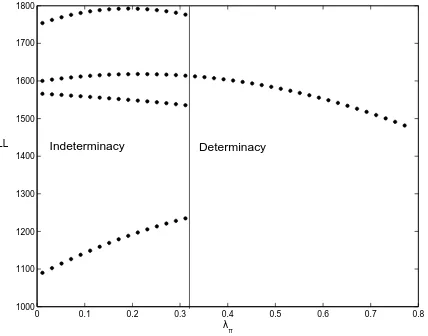
Figure (1) shows an example of multiple MSV solutions under indeterminacy. The Figure plots the log-likelihood function (LL) against the policy parameter λπ.

This example is constructed by perturbing the parameter set at the optimum in the direction of the response of the interest rate to inflation (i.e. all parameters except

λπare held constant). When the response of the interest rate to inflation is too weak,

(32)

0 0.1 0.2 0.3 0.4 0.5 0.6 0.7 0.8 1000

1100 1200 1300 1400 1500 1600 1700 1800

λ_π

LL _{Indeterminacy} _Determinacy

(33)

References

Altig, David, Lawrence J. Christiano, Martin Eichenbaum, and Jesper Linde (2003) ‘Technology shocks and aggregate fluctuations.’ mimeo

Andrés, J., J. D. López-Salido, and J. Vallés (2001) ‘Money in an Estimated Business Cycle Model of the Euro Area.’ Bank of Spain, working paper No. 0121 Basu, Susanto, John Fernald, and Miles Kimball (1998) ‘Are technology

improvements contractionary?’ FED, International Finance Discussion Papers No. 625

Blanchard, Oliver, and Charles M. Kahn (1980) ‘The solution of difference models

under rational expectations.’ Econometrica 48, 1305–1311

Calvo, Guillermo A. (1983) ‘Staggered prices in a utility-maximizing framework.’

Journal of Monetary Economics 12, 383–98

Cho, S., and A. Moreno (2002) ‘A Structural Estimation and Interpretation of the New Keynesian Macro Model.’ mimeo

Christiano, Lawrence J., Martin Eichenbaum, and Charles Evans (2001) ‘Nominal rigidities and the dynamic effects of a shock to monetary policy.’ NBER working paper w8403

Clarida, Richard, Jordi Gal´ı, and Mark Gertler (1998) ‘Monetary policy rules in

practice: Some international evidence.’ European Economic Review

42, 1033–1067

(1999) ‘The science of monetary policy: A New Keynesian perspective.’ Journal

of Economic Literature 37, 1661–1707

Deutsche Bundesbank (1995) The Monetary Policy of the Bundesbank (Frankfurt

am Main, Germany)

Evans, G. W., and S. Honkapohja (2001) Learning and Expectations in

Macroeconomics (Princeton, NJ: Princeton University Press)

Farmer, Roger E. A. (1999) The Macroeconomics of Self-Fulfilling Prophecies,

second ed. (MIT Press)

Gal´ı, Jordi, and Mark Gertler (1999) ‘Inflation dynamics: A structural

econometric analysis.’ Journal of Monetary Economics 44, 195–222

Gal´ı, Jordi, Mark Gertler, and J. David L´opez-Salido (2001) ‘European inflation

dynamics.’ European Economic Review45, 1237–1270

(34)

60, 65–99

Hamilton, James D., ed. (1994) Time Series Analysis (Princeton University Press)

Hoffmann, Johannes, Jeong-Ryeol Kim, and Hans-Georg Wels (2003) ‘Der Einfluss

der Euro-Bargeldeinf¨uhrung auf die Verbraucherpreise in Deutschland.’ mimeo,

Deutsche Bundesbank

Ireland, Peter N. (2002) ‘Money’s Role in the Monetary Business Cycle.’ mimeo, Boston College

(2003) ‘A Method for Taking Models to the Data.’ mimeo, Boston College Klein, Paul (2000) ‘Using the generalized Schur form to solve a multivariate linear

rational expectations model.’ Journal of Economic Dynamics and Control

24, 1405–1423

Kuntsevich, A., and F. Kappel (1997) ‘SolvOpt – The solver for local nonlinear optimization problems.’ mimeo, University of Graz, Austria

Lubik, Thomas A., and Frank Schorfheide (2002) ‘Testing for Indeterminacy: An Application to U.S. Monetary Policy.’ PIER working paper No. 02-025

McCallum, Bennett T. (1999) ‘Role of the Minimal State Variable Criterion in

Rational Expectations Models.’International Tax and Public Finance6, 621–639

(2002) ‘The unique Minimum State Variable RE solution is E-stable in all well formulated linear models.’ mimeo, Carnegie Mellon University

(2003) ‘Multiple-solution indeterminacy in monetary policy analysis.’ Journal of Monetary Economics 50, 1153–1175

McGrattan, Ellen R., Richard Rogerson, and Randall Wright (1997) ‘An

equilibrium model of the business cycle with household production and fiscal

policy.’ International Economic Review 38, 267–290

Rotemberg, Julio J. (1982) ‘Sticky prices in the United States.’ Journal of Political Economy 90, 1187–1211

Taylor, John B. (1993) ‘Discretion versus policy rules in practice.’

Carnegie-Rochester Conference Series on Public Policy 39, 195–214

Uhlig, Harald (1999) ‘A Toolkit for Analyzing Nonlinear Dynamic Stochastic

Models Easily.’ InComputational Methods for the Study of Dynamic Economies,

ed. Ramon Marimon and Andrew Scott (Oxford: Oxford University Press) chapter 3

Woodford, Michael (2003) ‘Interest and Prices: Foundations of a theory of

(35)

ξ ζ σ β

(whole sample) (1970:q1-1989:q4) (1970s) (1980s) (1993:q1-1989:q4)

0.8 1 1

0.9921 0.9926 0.9952 0.9900 0.9937

Table 1: Calibrated parameters

Whole sample estimate t-value

ρR 0.842 19.969

λy,t−1 0.079 3.03

λπ,t−1 0.399 5.347

λµ,t−1 0.081 3.336

λy,t 0.025 0.956

λµ,t -0.07 -2.457

λπ,t -0.309 -3.659

ρa 0.797 15.169

ρz 0.545 5.387

ρe 0.78 12.571

σa 0.02 3.442

σz 0.035 5.29

σR 0.002 10.482

σe 0.012 10.093

γ2 0.965 3.018

ω 0.949 5.063

γf 1 NaN

a

Log-likelihood 1808.3

a

The log-likelihood function is discontinuous to the right of this point esti-mate. The standard error are therefore not computed.

(36)

Whole sample 1993:q10-1998:q4 estimate t-value estimate t-value

ρR 0.81 21.768 0.755 13.596

λy 0.085 6.524 0.026 0.988

λπ 0.191 4.228 0.168 3.219

λµ 0.045 2.216 0 1.329

ρa 0.784 15.316 0.843 15.326

ρz 0.57 4.567 0.191 0.919

ρe 0.769 12.286 0.768 6.951

σa 0.021 3.565 0.022 2.874

σz 0.039 2.928 0.003 0.785

σR 0.002 14.93 0.001 6.473

σe 0.012 8.643 0.014 6.331

γ2 1.191 2.657 2.203 3.987

ω 0.808 4.559 0.609 5.934

γf 0.888 9.879 1 NaN

a

Log-likelihood 1792.50 420.01

a

The log-likelihood function is discontinuous to the right of this point esti-mate. The standard error are therefore not computed.

(37)

1970:q1-1989:q4 1970s 1980s estimate t-value estimate t-value estimate t-value

ρR 0.819 17.91 0.68 9.292 0.682 5.664

λy 0.072 3.156 0.116 3.93 0.089 3.612

λπ 0.221 3.943 0.489 3.858 0.41 2.689

λµ 0.085 3.641 0.106 2.675 0.154 2.9

ρa 0.751 12.79 0.597 5.997 0.417 1.954

ρz 0.407 2.558 0.585 3.3 0.224 1.007

ρe 0.65 6.987 0.54 3.679 0.75 7.01

σa 0.018 3.53 0.016 3.441 0.005 1.755

σz 0.049 4.21 0.04 2.658 0.049 2.864

σR 0.002 11.611 0.003 8.315 0.002 7.808

σe 0.012 8.1 0.012 6.677 0.012 3.733

γ2 1.143 3.122 1.1 2.53 1.02 1.561

ω 0.914 5.248 0.962 4.114 1.026 3.302

γf 0.846 14.619 0.84 9.493 0.857 6.778

Log-likelihood 1227.7 596.17 647.38

(38)

estimate t-value

ρR 0.79 19.698

λy 0.098 5.998

λπ 0.216 4.375

λµ 0.036 1.801

ρa 0.809 16.339

ρz 0.722 6.543

ρe 0.8 13.587

σa 0.022 3.431

σz 0.028 2.543

σR 0.002 13.93

σe 0.011 8.571

γ2 1.374 2.432

ω 0.739 3.851

γf 0.901 8.126

σy 0.005 4.295

σπ 0.001 2.058

σpolicy 0 0

σm 0 0

Log-likelihood 1795.5

(39)

Forecast horizon 1 4 8 12 16 ∞

output

preference shock 75.9 70.56 70.35 70.35 70.35 70.35

technology shock 4.73 10.56 10.87 10.88 10.88 10.88

policy shock 19.31 18.28 18.16 18.15 18.14 18.14

money demand shock 0.07 0.6 0.62 0.62 0.62 0.62

inflation

preference shock 4.41 5.68 5.96 6 6.01 6.01

policy shock 0.05 0.04 0.04 0.04 0.04 0.04

interest rate

preference shock 0 75.45 76.92 77.12 77.15 77.15

technology shock 0 10.17 9.66 9.58 9.56 9.56

policy shock 100 13.88 12.94 12.83 12.81 12.81

money demand shock 0 0.5 0.48 0.47 0.47 0.47

money balances

policy shock 21.93 18.5 18.14 18.1 18.1 18.09

(40)

output

policy shock 0.79 2.66 7.26 10.8 13.14 22.61

inflation

policy shock 25.01 29.29 28.49 27.96 27.64 26.67

money demand shock 0 0 0 0 0 0

interest rate

policy shock 100 62 45.59 38.9 35.58 27.95

money demand shock 0 0 0 0 0 0

money balances

policy shock 4.01 18.33 27.12 28.66 28.53 26.83

(41)

output

policy shock 0.42 14.02 19.59 20.65 21 21.73

inflation

policy shock 23.42 24.85 23.85 23.35 23.07 22.38

interest rate

policy shock 100 42.57 31.87 28.5 26.94 23.47

money balances

policy shock 9.93 25.76 26.07 24.88 24.2 22.66

(42)

output

policy shock 0.26 4.99 13.48 19.36 23.1 34.81

money demand shock 60.77 39.62 34.78 29.05 25 12.43

inflation

policy shock 25.37 39.8 41.76 42.48 42.86 43.81

interest rate

policy shock 100 58.38 51.73 49.54 48.47 45.91

money balances

preference shock 7.21 5 15.79 24.26 29.41 43.03

policy shock 3.49 16.28 25.7 30.75 33.47 40.18

(43)

5 10 15 20

Figure 2: Response of the economy to a policy shock.

5 10 15 20

(44)

5 10 15 20

Figure 4: Response of the economy to a productivity shock.

5 10 15 20

(45)

(46)

(47)

1970 1975 1980 1985 1990 1995 2000 −0.06

−0.04 −0.02 0 0.02 0.04 0.06

GDP M3

Figure 10: Detrended per capita output and real balances.

1970 1975 1980 1985 1990 1995 2000

−0.005 0 0.005 0.01 0.015 0.02 0.025 0.03 0.035 0.04

R−1 π

(48)

R2

parameter log-likelihood output money inflation interest rate

Model 10 (14) 1792.5 54% 78% 48% 89%

VAR(1) 20 1814.2 57% 79% 57% 92%

VAR(4) 68 1814.4 66% 82% 72% 94%

Table 10: Fit of the model in comparison to a VAR.

output money inflation interest rate

RMSE 0.0107 0.0075 0.0079 0.0059

Model

MAPE 116.97 79.17 121.24 26.99

RMSE 0.0121 0.0127 0.0049 0.0038

VAR(1)

MAPE 148.58 94.92 75.46 12.43

RMSE 0.0169 0.0221 0.0056 0.0078

VAR(4)

MAPE 116.67 230.44 84.641 26.36

(49)

1980 1981 1982 1983 1984 1985 −0.03

−0.02 −0.01 0 0.01 0.02 0.03 0.04

Actual and forecast values of output

actual forecast

1980 1981 1982 1983 1984 1985

−0.03 −0.02 −0.01 0 0.01 0.02

Actual and forecast values of money

actual forecast

19800 1981 1982 1983 1984 1985

0.005 0.01 0.015 0.02

Actual and forecast values of inflation

actual forecast

1980 1981 1982 1983 1984 1985

0.01 0.015 0.02 0.025 0.03 0.035

Actual and forecast values of interest rate

actual forecast

(50)

The following papers have been published since 2002:

January 2002 Rent indices for housing in West Johannes Hoffmann

Germany 1985 to 1998 Claudia Kurz

January 2002 Short-Term Capital, Economic Transform- Claudia M. Buch

ation, and EU Accession Lusine Lusinyan

January 2002 Fiscal Foundation of Convergence

to European Union inLászló Halpern

Pre-Accession Transition Countries Judit Neményi

January 2002 Testing for Competition Among

German Banks Hannah S. Hempell

January 2002 The stable long- run CAPM and

the cross-section of expected returns Jeong-Ryeol Kim

February 2002 Pitfalls in the European Enlargement

Process – Financial Instability and

Real Divergence Helmut Wagner

February 2002 The Empirical Performance of Option Ben R. Craig

Based Densities of Foreign Exchange Joachim G. Keller

February 2002 Evaluating Density Forecasts with an Gabriela de Raaij

Application to Stock Market Returns Burkhard Raunig

February 2002 Estimating Bilateral Exposures in the

German Interbank Market: Is there a Christian Upper

Danger of Contagion? Andreas Worms

February 2002 The long-term sustainability of public

finance in Germany – an analysis based

(51)

March 2002 The pass-through from market interest

rates to bank lending rates in Germany Mark A. Weth

April 2002 Dependencies between European

stock markets when price changes

are unusually large Sebastian T. Schich

May 2002 Analysing Divisia Aggregates

for the Euro Area Hans-Eggert Reimers

May 2002 Price rigidity, the mark-up and the

dynamics of the current account Giovanni Lombardo

June 2002 An Examination of the Relationship

Between Firm Size, Growth, and

Liquidity in the Neuer Markt Julie Ann Elston

June 2002 Monetary Transmission in the

New Economy: Accelerated

Depreci-ation, Transmission Channels and Ulf von Kalckreuth

the Speed of Adjustment Jürgen Schröder

June 2002 Central Bank Intervention and

Exchange Rate Expectations –

Evidence from the Daily

DM/US-Dollar Exchange Rate Stefan Reitz

June 2002 Monetary indicators and policy rules

in the P-star model Karl-Heinz Tödter

July 2002 Real currency appreciation in

acces-sion countries: Balassa-Samuelson and

investment demand Christoph Fischer

August 2002 The Eurosystem’s Standing Facilities

in a General Equilibrium Model of the

(52)

August 2002 Imperfect Competition, Monetary Policy

and Welfare in a Currency Area Giovanni Lombardo

August 2002 Monetary and fiscal policy rules in a

model with capital accumulation and

potentially non-superneutral money Leopold von Thadden

September 2002 Dynamic Q-investment functions for

Germany using panel balance sheet data

and a new algorithm for the capital stock Andreas Behr

at replacement values Egon Bellgardt

October 2002 Tail Wags Dog? Time-Varying Informa- Christian Upper

tion Shares in the Bund Market Thomas Werner

October 2002 Time Variation in the Tail Behaviour of Thomas Werner

Bund Futures Returns Christian Upper

November 2002 Bootstrapping Autoregressions with

Conditional Heteroskedasticity of Sílvia Gonçalves

Unknown Form Lutz Kilian

November 2002 Cost-Push Shocks and Monetary Policy

in Open Economies Alan Sutherland

November 2002 Further Evidence On The Relationship

Between Firm Investment And Robert S. Chirinko

Financial Status Ulf von Kalckreuth

November 2002 Genetic Learning as an Explanation of

Stylized Facts of Foreign Exchange Thomas Lux

Markets Sascha Schornstein

December 2002 Wechselkurszielzonen, wirtschaftlicher

Aufholprozess und endogene

Realign-mentrisiken * Karin Radeck

Money in a New Keynesian model estimated

Money in a New-Keynesian model estimated

with German data

Jana Kremer

Giovanni Lombardo

Thomas Werner

Discussion paper

Contents

List of Figures

List of Tables

Money in a New-Keynesian model

estimated with German data

∗

1

Introduction

2

The model

Households

Monetary policy

Exogenous disturbances

Reduced form of the model

3

Data

4

Estimation

The state-space form of the model and its solution

5

Results

5.1

Impulse responses

5.2

Variance decomposition

5.3

Empirical performance of the model

6

Conclusions

Appendix

A

ML estimation of a Linear Rational

Expecta-tion model using the MSV soluExpecta-tion

References

The following papers have been published since 2002: