Loss Averse agents in a New Keynesian DSGE
model
Francesco Simone Lucidi
Department of Economics, University of Rome "La Sapienza"
December 2, 2015
Abstract
The work is aiming at introducing behavioral assumptions in a New Keynesian fashion. We present a baseline NK-DSGE where …nancial hold-ings are assumed to enrich agents’ preferences through a state-dependent function re‡ecting Prospect Theory phenomena. The model creates a more volatile dynamics of the real variables along the business cycle. In particular, for an exogenous positive monetary shock, households tend to accumulate less …nancial activities and consume more in respect to stan-dard NK-DSGE.
Introduction
This work strives to object the state "everything becomes possible when we move into the territory of irrationality" by introducing Prospect Theory elements into a standard New Keynesian DSGE model (NK-DSGE). This idea comes from the belief that once macroeconomists consider totally the notion that individu-als have cognitive limitations and are not completely capable to understand the complexity of the world it is possible to develop dynamic models based on di¤er-ent notion of rationality which are more in line with the reality of the world. The model this work presents does not desires to provide an exhaustive representation of the world neither illuminating predictions on …nancial markets or monetary policy. It simply provides a portable extension of a standard NK-DSGE where the concept of rationality of agents is reinterpreted by changing the standard utility function. In particular, the innovating assumption is that, apart standard consumption and labor supply decisions, each period households evaluate the state of their …nancial wealth returns and when they experience a loss their disu-tility is worst in respect to the well-being experienced from an equivalent gain. These are state-dependency and loss aversion phenomena predicted by Prospect Theory.
The work is structured as follow: the …rst section presents a brief review of Prospect Theory literature and its usages in macroeconomics. In section 2 a NK-DSGE model containing Prospect Theory assumptions is illustrated (LANK model). The main implications and performaces of such a model are pintpointed in Section 3. Concluding Section discusses all the results of the LANK model.
shock, households tend to accumulate less …nancial activities and consume more in respect to standard NK-DSGE.
1
Prospect Theory foundations and its
macro-economics’ usages
Launching PT in 1979, the two Israeli psychologists Kahneman and Tversky (KT) aimed to create an alternative to expected utility theory. Providing a solid experimental basis, they noticed choices among risky prospects exhibit several pervasive e¤ects which are inconsistent with the fundamentals of pre-existing utility theory. KT found empirically that people underweight outcomes that are merely probable in comparison with outcomes that are obtained with certainty (certainty e¤ect). This e¤ect contributes to people’s risk aversion for choices involving sure gains and to risk seeking for choices involving losses. Even though the article of 1979 presents all the experimental bases of PT and alternative model insights, it su¤ers of some limitations: it can be applied to gambles with at most two non-zero outcomes, and it predicts people sometimes choose domi-nated gambles (Barberis N., Thirty Years of Prospect Theory in Economics: A Review and Assessment, Journal of Economic Perspectives, 2013). However, a modi…ed version of PT was published in 1992 by KT called “cumulative PT” which overcomes both problems and it is still the most used version in economic theories.
In order to show brie‡y the main di¤erence between expected utility theory (EUT) and PT consider the gamble:
(x m; p m;x m+1; p m+1;:::;x0; p0;:::;xn 1; pn 1;xn; pn)
wherep’s are the probability that x’s gains occur. If W is de…ned as current wealth and U( ) is a concave utility function, then under EUT as individual evaluates the gamble as:
n
X
i= m
piU(W +xi)
Instead, under cumulative PT the gamble is evaluated as:
n
X
i= m
iv(xi)
where v( ) is called the value function and it is increasing with v(0) = 0, and where i are said decision weights. Through this formulation all main four
aspects of PT emerges: 1) reference dependence 2) loss aversion 3) diminish sensitivity and 4) probability weighting. The …rst property comes to the fact that, under PT, people assess their utility (or disutility) —deriving from gains and losses— looking a certain reference point, thus the absolute level of wealth does not enter in their evaluation process1.
Secondly, loss aversion implies also small losses worth more than gains of equivalent magnitude. As a result, the value function is displayed steeper in the region of losses than in region of gains. KT infer loss averse agents from the fact
that these turn down the gamble(100$;1 2; 110$;
1
2)because the pain of lose 100$ far outweighs the pleasure of winning 110$.
Third, diminish sensitivity implies that the value function is concave in the region of gains but convex in the region of losses: it means people’s evaluation of gains (or losses) changes according with the relative distance from the reference point. Thus, while replacing a 100$ gain (or loss) with a 200$ gain (or loss) has a signi…cant utility impact, replacing a 1,000$ gain (or loss) with a 1,100$ gain (or loss) has a smaller impact. This property motivates the concavity (convexity) over gains (over losses): people tends to be risk averse over moderate probability gains and risk seeking over losses.
The last property of PT implies people do not weight outcomes by objective probabilities pi, but they use decision weights i. In KT 1992, the latter are
assessed through a speci…c function w( ) whose argument is an objective prob-ability. Probability weighting leads the individual to overweight the tails of any distribution, so to overweight unlikely extreme outcomes: KT …nd that people prefer 0.001 chances of 5,000$ to a certain gain of 5$, but at the same time they prefer a sure loss of 5$ rather than 0.001 chances of losing 5,000$. However, this would not be considered a fallacious rationality, but simply it is agents’ rationality which —as data speaks— hardly takes shape as EUT predict.
Despite these phenomena have paved the way for a new vein of research, few economists have undertaken the study of PT. Indeed, the central idea of PT is that people derive utility from gains and losses in respect with a reference point, but in any given economic context it might be di¢cult to de…ne what gains and losses are and how to de…ne the reference point. This might depend on several aspects such as agents’ beliefs, their starting points, the context in which they choose or their expectations about the future. Fortunately, some researchers have tried to understand how people conceptualize gains and losses in di¤erent contexts. The main approach researchers are taking is to derive PT predictions by de…ning before a variety of de…nitions of gains and losses that then are tested both in laboratory and in theoretical …eld. Similarly to De Grauwe, Rabin and Koszegi2 have argued that the reference point people use to evaluate gains and
losses is their expectations (or beliefs) held in the recent past about outcomes. These authors also emphasized the fact that what matter is not to replace EUT assumptions with PT assumptions in the models, but rather to …nd out whether it is useful to consider models where people derive utility from both gains and losses and, as in traditional analysis, from consumption levels.
Anyway, PT have found room in several economic …elds, above all …nance3
, insurance4 and consumption-saving decisions5, but also in labor supply6,
in-dustrial organization7 and principal-agent bargaining8. Of course, here will be
brie‡y discussed few of these …elds coherently with the aim of the work.
22006, 2007 and 2009.
3Benartzi and Thaler’s, 1995, Barberis, Huang, and Thaler, 2006, Barberis and Huang,
2008 Green and Hwang, 2012, just to quote few.
4Hu and Scott, 2007 but also Sydnor, 2010. 5K½oszegi and Rabin, 2009 but also Pagel, 2012b. 6Camerer, Babcock, Loewenstein, and Thaler, 1997. 7Heidhues and K½oszegi, 2012.
1.1
Key applications and empirical issues of Prospect
The-ory
Being a model of decisions making under risk, PT is naturally suitable for ex-plaining …nancial phenomena. Indeed, …nance is the …eld where PT has been most applied, especially in three areas: the cross section of average returns, won-dering why some assets have higher returns than others, the aggregate stock market and lastly the trading of …nancial assets over time.
Barberis and Huang face the …rst issue by using PT utility, assuming that agents evaluate the changes of the value of their portfolios over the course of one period. In this model PT leads to a new prediction on the evolution of assets’ prices, which is that a security’s skewness (non-symmetry) in the distribution of its returns is priced. In particular, positively skewed security (means it gives fre-quent small losses and few extreme gains) will be overpriced (in respect with the price that would prevail in a system with expected utility investors) and it will earn a lower average return. This e¤ect is a consequence of probability weighting by investors who tend to overweight the tails of the distribution they are consid-ering: here, they overweight the unlikely state of the world in which they may make money by investing in the positively skewed stock. One interesting feature of this prediction is that it appears to be robust to di¤erent ways of de…ning what a gain or loss means to investors9 and moreover it …nds also a signi…cant
empirical support10. Pricing skewness predicted through PT has been used by
many researchers to address several …nancial phenomena: the low average return of distressed stocks, of bankrupt stocks, of stock of traders over-the-counter, to say few.
Further, the aggregate stock market is the best-context in which PT has been applied in …nance: Benartzi and Thaler (1995) stress the idea that loss aversion can explain the so called equity premium puzzle, the empirical evidence that the average return of US stock market systemically exceeds the average return of Treasury bills by a margin greater than the one predicted by traditional consumption-based models of asset prices. This is due to the fact that investors is assumed to consider the historical distribution of annual stock market returns, thus if the latter are highly dispersed they will be retained unappealing— because of loss aversion. In order to compensate this discrepancy, the stock market needs to maintain average return more desirable than a safe Treasury bills. Moreover, the reasoning exploits not only PT but also another concept that the authors callnarrow framing meaning an individual evaluates a risk separately from other risks he faces11. Furthermore, several works support and proved empirically the
idea that both loss aversion and narrow framing are able to explain also the so called non-participation puzzle, the fact that most households do not participate in the stock market12. The idea of narrow framing together with loss aversion
will represent the ground of the behavioral assumptions proposed into the model presented in the next section.
The last strand of PT usage in …nance regards how people trade assets over time. Researchers have investigated the so called disposition e¤ect, the evidence that investors tend to sell assets which have raisen their value in last periods rather than assets performing worst13. According with EUT this behaviour is
9see Barberis and Huang, 2008.
10Boyer et. al. (2010) found positively skewed stocks will have lower average returns. 11see Benartzi and Thaler, 1995
inconsistent, investors should orientate their selling on stocks presenting poor past performance, but evidences show they do the opposite. On the contrary, PT simply can explain this behaviour because of the convexity of the value function in the region of losses14. Indeed, using PT, when a stock turn up in the
region of losses, the loss averse individual becomes risk-seeking and he tends to hold the stock until it performs better.
Despite the original …eld of application of PT some authors as Thaler (1980) argued that PT can be used in a riskless environment also. KT (1991) and Koszegi and Rabin (2006) tried to interpret PT in this sense assuming individu-als derive utility from current consumption relative to some reference level, and that utility function presents both loss aversion and diminishing sensitivity. The experimental ground of this phenomenon is called endowment e¤ect, which in turn refers to two di¤erent …ndings: initial allocation has a huge e¤ect on subse-quent choices (exchange asymmetries) and the asymmetry between willingness to pay and willingness to accept. More speci…cally, the former refers to an ex-periment of Knetsch (1989) in which half of partecipants receive a mug and the other half a candy, then it is asked whether they want to exchange the object they received for the other. The result was 89% of partecipants receiving a mug opt to keep it, while 10% of partecipants receiving a candy opt to exchange it with a mug. Of course, EUT predicts preferences over goods do not depend on the initial endowment. Meanwhile, the second e¤ect refers to an experiment made by Kahneman, Knetsch, and Thaler (1990) in which half of partecipants receive initially a mug and the other half nothing. In the second step both groups receive an equal list of prices, then the …rst group of partecipants have to chose singularly their willingness to accept money in exchange of their mug and the other group their willingness to pay that mug. The result shows the median price for accepting the exchange is 5.75$ while the median willingness to pay is 2.25$. Therefore, both experiments are signed by the e¤ects of loss aversion: in the …rst experiment partecipants perceive the exchange as a "loss" in respect with their initial "gain", in the same way, in the second experiment partecipants perceive as a "loss" to give up the mug. However, List (2003, 2004) conducts the same kind of experiment but with partecipants including dealers (people who trade often and professionally) and non-dealers. His results show that dealers are more willing to exchange objects of an equivalent value, and this suggests PT might be less useful in describing experienced economic actors’ behaviour15.
Following this strand, Koszegi and Rabin (2009) tried to incorporate PT into a dynamic model of consumption choice. At each instant of time individuals de-rive utility from two sources: one is the di¤erence between present consumption and the expectation on present consumption assessed recently, the other the dif-ference between the individual’s currently projected consumption at each future date and the consumption that person recently expected at that date. This util-ity incorporates loss aversion so that individuals are more sensitive to bad news in respect with good news about their expected consumption. A framework like this a¤ects precautionary saving: current uncertainties about consumption positively a¤ect current savings as to reduce expected pains. On the other side, when there is less uncertainty individuals tend to over-consume, because each period they have an incentive to surprise themselves with a little extra-consumption. These
14see Shefrin and Statman, 1985.
15However, Koszegi and Rabin (2006) argue this result might be consistent with PT if a
predictions are both consistent with the evidence that consumption appears to adjust insu¢ciently to income shocks (excess sensitivity and excess smoothness puzzles) so that when negative shocks occur individuals prefer to lower future consumption rather than current consumption.
1.2
New Keynesians and the behavioral challenge
During the last decades, many NK scholars have tried to enlarge macroeconomic research’s frontiers by incorporating behavioral hypotheses in their models. Tak-ing in mind the guidelines of NK thought, a …rst reason of such tendency is in-stantly clear: the more economic human behaviors are pinpointed and supported by experimental evidences, more chances to micro-found there are. Therefore, more realistic hypotheses on agents should provide a more solid ground to ex-plain macroeconomic tendencies shown by the data. On the other hand, part of NKs involved in this arena are prompted to introduce behavioral hypotheses in order to overcome the de…ciencies of baseline models. Indeed, as acknowledged, even though baseline NK-DSGE has been successful in explaining broad features of the response of real variables to monetary policy, they lack of inertia of macro-economic variables: shocks have immediately e¤ects and dissipate quickly. This prediction is strongly denied by empirical evidences showing, as instance, that the e¤ects of monetary policy shocks are lagged and long-lasting.
Shortcomings like this have largely involved NKs to explore di¤erent mod-els of consumption (given the formulation of the NKIS curve), di¤erent ways of thinking of expectations formation, or di¤erent models of nominal wage de-termination. However, despite the spreading trend to incorporating behavioral hypotheses in NKs’ models, literature does not present many NK’s attempts to exploit PT’s assumptions in macroeconomics models.
Two recent papers of Ciccarone et al.16 contribute to enrich the assumption
of loss averse agents in macroeconomic models, and their peculiarities allow to …nd a landmark for this work. In the …rst work the authors explain how to intro-duce elements of PT in a standard general equilibrium overlapping generations economy with monopolistic competition in the goods market. This model shows that increasing loss aversion of agents may have two opposite e¤ects: on one hand, it decreases the wage mark-up which in turn leads to an higher equilib-rium output (and lower equilibequilib-rium wage). On the other hand, it makes agents more cautious in supplying labour, and thus this lowers the equilibrium output. If the former e¤ect is stronger than the latter, then higher imperfect rationality would increase equilibrium employment and potential output.
In the second work, the researchers try to add elements of PT in a Lucas’ “is-lands” model. Here, they include reference dependence, diminish sensitivity and loss aversion in agents’ utility function following Barberis et. al. (2001) where the representative agent derives utility not only from consumption levels but also on change in the value of her …nancial wealth. Futher, the resulting utility function states at present time agent cares about both her expected consumption level of the next period and her expected real …nancial wealth in respect with a reference point. The function governing the latter expectation accounts for loss aversion – thus, it lowers agents utility – when expected agents real …nan-cial wealth lies below the reference point which is assumed real money holdings. Therefore, the reference point is taken as amount of real assets obtained if no monetary shock occurred. More speci…cally, when the expected stochastic gross
rate of return on real wealth is greater than or equal to one (monetary shock) the agent is obtaining a gain and, thus she does not display any future loss that would lower the value of her expected utility. The model presented in the next section will borrow the state-dependent preference within the utility function in a similar way.
Finally, a recent attempt to incorporate PT in a NK-DSGE was made by Ga¤eo E. et. al17: the novelty of their work is to embed PT de…ning
state-dependent preferences in a dynamic NK framework in order to explain the trans-mission of monetary policy to output and in‡ation. Their model involves PT consequences for both consumption demand and labor supply. In particular, the assumption of loss averse preferences in consumption allows the researchers to explain the asymmetric e¤ects of monetary policy on output over di¤erent cyclical phases and, for the same reason, symmetric responses of in‡ation. This behaviour would be due to a double e¤ect induced by loss aversion: on one hand, during contractions households tend to have an increased elasticity of intertem-poral substitution between current and future consumption. On the other hand, loss aversion implies also state-dependent marginal rate of substitution between consumption and leisure that in turn makes the labour supply schedule ‡atter below the reference point creating a downward stickiness of real wages during contractions. Therefore, changes in real interest rate would exert a stronger im-pact on output in respect with expansive phases, but the same e¤ect cannot be appreciated on in‡ation due to the real rigidity on the labour market.
2
A New Keynesian DSGE model with loss averse
agents
The presented model consits in a baseline NK-DSGE where …nancial holdings are assumed to enrich agents’ preferences through a state-dependent function re‡ecting PT phenomena. This model will be called Loss Averse New Keynesian DSGE model (LANK-DSGE or LANK). In particular, apart consumption and leisure, each period agents care for departures of real …nancial wealth —deriving from bonds that they held— from a reference point taken as amount of real assets when no monetary shock occurs. This assumption has a similar shape of the phenomenon explained before of narrow framing, thus each period agents consider …nancial gains’ changes as a part of their utility. The function describing this innovation contains also another elements of PT such as loss aversion (KT, 1992) which in general consider individual evaluations under risk strictly a¤ected by both their state-reference level and the magnitude of changes from that point so that agents account more for losses than for equivalent gains.
The innovation on the utility function does not allow for any other depar-ture from a baseline NK-DSGE. Therefore, in order to better appreciate state-dependent preference implications both …rms and Central Bank (CB) are as-sumed to behave as in the Galì’s baseline (2008).
2.1
Households
The model assumes a representative in…nitely-lived household seeking to maxi-mize its life-time utility de…ned as follow:
E0
quantity of good i 2 [0;1] consumed by household in period t. Household’s period budget constraint is then:
Z 1
0
Pt(i)Ct(i)di+QtBt Bt 1+WtNt+Tt
where: Pt(i) is the price of good i, Nt are hours worked, Wt is the nominal
wage, Bt are one-period bonds purchased at price Qt and Tt is a lump-sum
component of income (e.g. dividends from ownership of …rms). For any give level of expenditure, the household demand an optimal quantity of any good
i2[0;1]which is given by:
Ct(i) =
Pt(i)
Pt
Ct (1)
Where Pt is the aggregate price level. This condition implies that total
con-sumption expenditure must equal price index times quantity index: Z 1
0
Households’ expected life-time utility is assumed to contains standard CRRAs for consumption and labor supply, while the innovation is in the additive function accounting for state-dependent preference:
The parameter k measures the importance of gains and losses in the utility function. The agent is not only loss averse (losses are more salient than gains), and subject to reference dependence, but also susceptible to some form of narrow framing: when evaluating …nancial wealth, she considers it per se, in addition to the expected utility of the consumption it can produce. Notice that this parame-ter will be useful to compare this model with baseline NK-DSGE, therefore it is assumed thatk is worth0when agents are "ultra-rational" and behave following EUT prescriptions, meanwhile when k >0 agents take care for displacements of returns on …nancial assets from the reference point. In this latter case, function
f( )takes place: it depends on the di¤erence between the households’ real value of assets considering monetary policy innovations occurring at time t, Bt
Pt(1 +it), and the real value of assets at timetwhen no monetary shock occurs, Bt
Pt(1 +r
n),
which is the reference point. More speci…cally, denoting Zt that di¤erence and
assuming the rate of return equals the rate of interest set by the CB, it follows:
Zt=
where rn denotes the wicksellian steady-state interest rate of the economic
system. Therefore, starting from the steady-state, when the CB implements an expansionary (restrictive) monetary policy lowering (increasing) the short-term interest rate Xt < 0 (Xt > 0) and hence the agents’ preference would be below
the reference point, Zt < 0 (Zt > 0). This mechanism makes function f(Zt)
state-dependent and assumes the following shape18:
f(Zt) =
Bt
PtXt ; Zt 0
Bt
PtXt ; Zt<0
where the parameter > 1 accounts for agents’ loss aversion. Therefore, if CB implements an expansive (contractive) monetary policy lowering (increasing) the rate of interest —shifting the value of households’ …nancial wealth below (be-yond) the reference point — function f(Zt) reduces (increases) utility function.
Furthermore, loss aversion hypothesis implies equivalent sized monetary policies of opposite sign make f(Zt) weightiness greater below the reference level than
beyond.
The representative household has to optimize its utility function subject to the budget constraint described by the following equation:
Ct+
Summarizing, when parameter k = 0, no preference on …nancial assets takes place and the baseline NK-DSGE is restored. When parameter k > 0 then household’s utility is a¤ected for some degree of a state-dependent preference represented by f(Zt). In the next section this property will be investigated
18This function has a similar shape of the one de…ned in Ciccarone G. and Marchetti E.
deeply. At this stage of analysis it is su¢cient to consider that when k >0 the Loss Averse New Keynesian DSGE model (LANK-DSGE) takes place by showing some source of narrow framing.
WhenZt 0, households’ …nancial assets are yielding higher returns due to a
restrictive monetary policy (CB applies an interest rate higher than the natural rate) and households’ utility is positively a¤ected. When Zt<0, it means CB is
implementing a monetary policy which lowers the interest rate below its natural (wicksellian) level of steady-state (Xt < 0). In this case loss aversion occurs
and parameter enters in households’ preferences: the loss on …nancial returns (represented by lower returns in respect with the one ensured by the natural rate) negatively a¤ects household’s utility. Therefore, there will be two optimal solutions for households depending on monetary shocks a¤ecting the economy. The following are the twoLagrangians occurring in the case of states beyond the reference point and below the reference point, respectively:
L =
From household’s maximization problem the following …rst order conditions are obtained for consumption, labor supply and bonds demand respectively:
t= tCt (2)
Equation (4) represents the optimal condition on bonds. It takes two di¤erent values according to the reference state. Therefore, state-dependency implies that the direction of monetary policy’s action a¤ects assets’demand. Moreover, by replacing equation (2) in conditions (4) two di¤erent Euler equations are obtained. Actually, the only di¤erence between the two consists in the parameter re‡ecting loss aversion. Hence, to make notation easier, it will be said that if Zt 0 than the following equation (5) presents = 1 and it describes the
upper-Euler equation, meanwhile, when Zt <0 equation (5) presents >1 and
describes the lower-Euler equation:
Ct = Ct+1 Pt Pt+1
(1 +it) +k (it rn) (5)
ct =Et(ct+1) 1
[it Et( t+1) +rn+k C (it rn)] (6)
This last is a log-linear approximation describing the dynamics of consump-tion along the optimal path19.
2.2
Firms
On the …rms’ side, the model proposed presents the same structure of a baseline NK model (Galí J., 2008). Therefore, there are a continuum of monopolystically competitive …rms producing di¤erentiated goods, indexed by i2[0;1]. Technol-ogy available in the system is the same for each …rm, thus they face the same production function:
Yt(i) = AtNt(i)1
WhereAtis the technology evolving exogenously over time. A key assumption
is that …rms are not able to adjust prices any time, so that they take into account of this in their decision-making process. According to Calvo rule (1983), only a fraction 1 ! of …rms will be able to adjust their prices any given period, where
! 2[0;1]is the index of price stickiness. Therefore, the aggregate price dynamic is de…ned as follow:
Pt = !(Pt 1)1 + (1 !) (Pt)
1 11
(7)
where, the price index is de…ned as Pt
hR1 the gross in‡ation rate as t PPtt1, the log-linearized version around the
steady-state of the (7) is obtained:
t= (1 !) (pt pt 1)
This last makes clear that in‡ation depends from the fact that …rms reopti-mizing in any given period choose a price that di¤ers from the economy’s average price of the previous periods. Therefore, in order to understand the in‡ation dy-namics one should analyze the features of the …rms’ decision-making process.
The representative reoptimizing …rm have to choose the price Pt
maximiz-ing the current market value of pro…ts generated by that price. Formally, the optimization process is shaped as follow:
max
subject to the sequence of demand constraints:
Yt+k=t =
a …rm that has reset its price in t. The maximization problem gives the follow …rst order condition:
1
…rm resetting its price in t, and M 1 . Notice that, whether all …rms can reset their price (no price stickiness and then ! = 0) the condition collapses to the traditional price-setting rule under ‡exible prices: Pt = M t=t. Thus, M
may be interpreted as desired mark-up (no frictions mark-up). However, the log-linearization of the optimal condition (8) around the zero in‡ation steady-state combined with market clearing conditions will lead to the NKPC describing the in‡ation dynamics. This procedure will be clari…ed in the next paragraph. Before to do this, consider M Ct+k=t Pt+t+k=tk the real marginal cost in t+k of
…rm adjusting its price in t, which in steady state is worth M C = 1=M, thus the log-linearization of the (8) gives:
pt pt 1 = (1 !)
As usual in standard NK models, market clearing in goods market requires
Yt(i) = Ct(i) for all i 2 [0;1] in any t. Being the aggregate output de…ned
, it follows that any t should hold:
Yt=Ct (10)
The log-linearized version of the (10) will be simply yt =ct, hence, the …rst key
equation of the system is obtained by replacing this last into the (6), the Loss Averse New Keynesian IS (LANK-IS) equation of the system:
yt=Et[yt+1]
1
(it Et[ t+1] +rn) +k C (it rn) (11)
which can be written also in terms of output gap:
xt=Et[xt+1]
1
(it Et[ t+1] +rn) +k C (it rn) (12)
where xt = yt ytf is the di¤erence between percentage deviations from
steady-state of current output and potential output (that is a second best due to monopolistic competition).
The market clearing condition on labor market requires Nt =
R1
0 Nt(i)di that combined with the production function …rms face, single good demand and goods market clearing condition, becomes:
Through the latter a relation between aggregate output, employment and technology is obtained20:
yt=at+ (1 )nt
This may be substituted in the relation for an individual …rm’s marginal cost in terms of the economy’s average real marginal cost:
mct = (wt pt) mpnt = (13)
= (wt pt) (at nt) log (1 ) =
= (wt pt)
1
1 (at yt) log (1 )
de…ning the economy’s average marginal product of labor in a way consistent with equilibrium condition. Next by exploiting the fact that mct+k=t =mct+k+
1 yt+k=t yt+k and equation (13), after tedious substitution, the relation (9) may be rearranged as the di¤erence equation:
pt pt 1 = !Et pt+1 pt 1 + (1 !) mcct+ t (14)
where = 1
1 +" 1. Notice that combining the (14) with relation t =
(1 !) (pt pt 1) it gives:
t= Etf t+1g+ mcct (15)
where (1 !)(1! !) is strictly decreasing in the index of price stickiness
!, in the measure of decreasing returns and in the demand elasticity ". This last relation highlights clearly that in NK’s models the in‡ation results from the aggregate consequences of price-setting decisions of …rms which are based on current and anticipated cost conditions. In the light of a further relation between economy’s real marginal costs and the level of aggregate economic activity the following relation can be obtained21:
c
mct = +
'+
1 yt y
f
t (16)
Finally, combining the (15) and the (16) the NKPC relating in‡ation to its one period ahead forecast and the output gap xt is obtained:
t= Etf t+1g+dxt (17)
whered +'1+ . The NKPC together with equation (12), the LANK-IS, represent the two key equations of the model.
The last equation closing the model is the rule that the monetary authority (CB) implements in order to control the ‡uctuations of the key macroeconomic variables of the system. This corresponds to implement a policy rule setting the short interest rate such that when exogenous shocks perturb the system it guarantees a unique path to achieve dynamically the equilibrium.
20There is also the termdt= (1 ) logR1
0
Pt(i)
Pt "
1
which is proved to be equal to zero up to a …rst order approximation in a neighborhood of the zero in‡ation steady-state (see Galì J., 2008).
In the next section di¤erent Taylor rules will be compared and the values of the weights that CB applies on its target will be changed in order to test the robustness of the LANK model. However, in the …rst step the simplest Taylor rule is implemented:
it= t+ xyt vt (18)
where and x are the weights that CB attributes to its targets of in‡ation and output gap respectively, and vt is an exogenous stochastic component with
zero mean. By construction, it is expected this rules should generate di¤erent re-sults between the LANK-DSGE model and the baseline NK-DSGE model. This is due to the fact that in the former CB has to consider the double e¤ect that the short term interest rate has on households’ utility: on one hand it changes the intertemporal choices on consumption as in baseline NK-DSGE. On the other hand, new short term interest rates change the dynamics of …nancial gains and this in turn a¤ects households’ utility due to some degree of narrow framing. Thus, when …nancial returns are far from the reference point households experi-ence a sort of adverse feeling to behave as in maximizing rationality. Moreover, due to loss aversion the e¤ect of narrow framing impact utility strongly when the CB action leads households’ …nancial preferences in the region of losses than when it leads in the region of gains.
In the next section the LANK model will be simulated through di¤erent Taylor rules and the e¤ects of these will be compared. However, this simple rule is a good starting point to understand which are the consequences of the LANK model.
2.4
Calibration
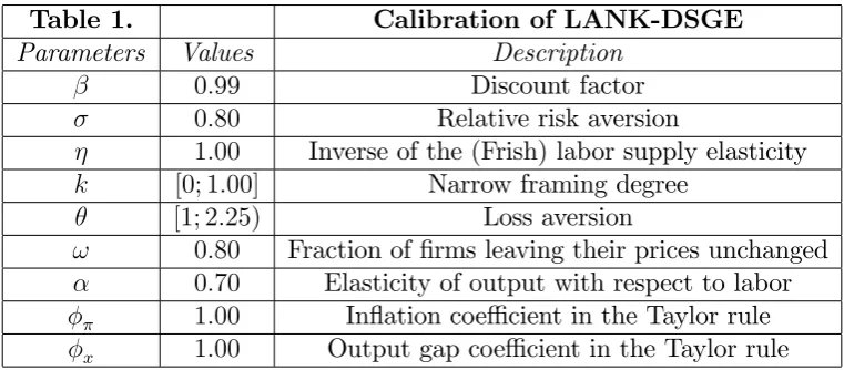
The calibration of the model follow the guidelines of both baseline NK-DSGE model22 and PT studies23. Table 1 summarizes compactly the values assumed for
di¤erent parameters. The time period corresponds to a quarter. With regard to preferences parameters, the coe¢cient of relative risk aversion equals 0:8, the inverse of Frish elasticity of labor supply equals 1 and the discount factor is set equal to 0.99. The parameter accounting narrow framing k will be tested for several values in a set[0;1]. According to KT (1991) the loss aversion parameter is set equal to 2.25 when a loss is experienced (the interest rate is below the reference point) and 1otherwise (interest rate is beyond the reference).
On the …rms’ side, the fraction of …rms unable to adjust prices ! equals 0.8 and the elasticity of output equals 0.7. Notice that the presence of just one steady-state value in the log-linearized version of the Euler equation, which is the term C , allows to normalize it to one rather than to try to …nd recursively all steady-state solutions of the variables. Finally, the weights that the CB applies on its targets and x are …rstly set to 1 both of them, and in such a way the Blanchard and
Khan conditions are already guaranteed as will be shown in the next section.
22Galì J., 2004.
Table 1. Calibration of LANK-DSGE
Parameters Values Description
0:99 Discount factor
0:80 Relative risk aversion
1:00 Inverse of the (Frish) labor supply elasticity
k [0; 1:00] Narrow framing degree
[1; 2:25) Loss aversion
! 0:80 Fraction of …rms leaving their prices unchanged 0:70 Elasticity of output with respect to labor 1:00 In‡ation coe¢cient in the Taylor rule
3
LANK-DSGE robustness, improvements and
further implications
In this section the implications of the LANK model are investigated. The aim is to test the robustness of the model highlighting the main departures from standard models’ implications when the behavioral hypothesis takes place. This step is crucial for the purpose of the work: bringing psychological assumptions in a standard environment and create a model where the same conventional tech-niques can be used. The need to have tractable models assumes particular impor-tance in the vein of behavioral economics in order to in‡uence prevalent models from their applied theory to econometrics, reduced-form and empirical works. This is the crucial point of Rabin24 who stressed the idea that the approach of
researchers to improve the realism of economic theories should be devoted to pro-duce models which are portable extensions of existing models (PEEMs). In the LANK model this idea might be tested through the investigation of parameter k
of narrow framing. Therefore, the …rst paragraph of the section will be devoted to test the predictions of the model as the parameter k changes.
Another important step for testing the LANK model is to investigate the implications of the behavioral hypothesis for monetary authority, so how the latter works when agents present both narrow framing and loss aversion and what happens when CB changes the weights on in‡ation target or when an empirical monetary policy rule takes place.
Lastly, in the …nal paragraph a speci…cation of the LANK model with a dif-ferent reference point is presented. In particular, it will be take in consideration that individuals compare current returns with the returns of the previous period looking at the one-period-before interest rate.
3.1
Is the LANK a PEEM?
The LANK model presents the basic structure to involve narrow framing and loss aversion in a NK-DSGE in an as much as possible simple way. In order to make further improvements of the model one should be able to turn back to the standard situation simply by resetting the parameter controlling the behavioral hypothesis. This is what Rabin call the capacity of the model to be PEEM. More precisely he argues researchers —whose aim is to incorporate psychological assumption in a comprehensive economic theory — must extend the existing model by formulating a modi…cation that embeds it as parameter values with the new assumptions as alternative parameter values, and make the model portable by de…ning it across domains using the same independent variables of existing research.
The LANK model satis…es all these condition by construction: all the vari-ables of standard NK-DSGE are involved, the parameterkcontrols the behavioral assumptions and by lowering it up to zero you may restore all the standard fea-tures of NK-DSGE model. Therefore, the fact that this model is a PEEM was already clear since the de…nition of the LANK-IS schedule. Now, this statement can be tested by perturbing the system through exogenous stochastic shocks and comparing the responses of the main variables of the LANK model and the standard NK-DSGE.
Here a positive monetary shock is considered . The non-systematic compo-nent of the interest rate follows an AR(1) process:
vt = vvt 1+"vt
where the exogenous shock "v
t is an i.i.d. and "vt N(0;0:02) and v =
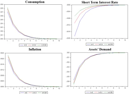
0:5. Figure 1 shows the percentage displacement from the steady-state of the interest variables in the LANK model. When k = 0 there is no framing and the e¤ects of the shock are the same of the baseline NK-DSGE (blue line). A positive (negative) realization of "v
tshould be interpreted as a contractionary
(expansionary) monetary policy shock leading to a rise (decline) in the nominal interest rate, given in‡ation and the output gap. The resulting increase of both current consumption and in‡ation is dampen by the control of short term interest rate which a¤ects both the aggregate spending and agents’ expectations, leading the system in steady-state within ten periods after the shock.
Next the narrow framing is introduced. Now when hit by a monetary shock the LANK model continues to display all the features of the previous case. Figure 1 shows that di¤erent degrees of narrow framing (k = 0:4 and k = 0:99, respec-tively signed by the red and the green lines) preserve a proportional relation, thus the degrees of narrow framing are neutral each other in terms of variables’ trends.
By introducing narrow framing the di¤erence is that lower …nancial returns induce agents to consider the loss they are experiencing separately from other choices. This change in agents’ optimal choices in turn a¤ects the entire dynamic of the system. The demand for …nancial assets lowers more than before: the e¤ect that households …nd more convenient to consume today rather than to shift resources in the near future is magni…ed. As a consequence the Taylor rule implies a more severe response of the CB which contains more interest rate ‡uctuations in respect with the previous case.
Therefore a …rst result of the LANK model arises: when narrow framing is activated it strengthens the responses of the main variables normally involved in a baseline NK-DSGE model hit by a monetary shock. This occurs because agents present a state-dependent preference for returns on …nancial activities which are compared with the returns they gain when the economy is in the steady-state.
Figure 1: The E¤ects of Narrow Framing.
3.2
LANK model and monetary policy rules
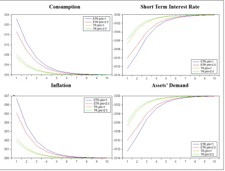
In order to make some robustness test this paragraph presents several simulations of the LANK model by implementing di¤erent speci…cations of the monetary policy. Figure 3 shows four simulations for a positive monetary shock using a neutral value of k = 0:99. The orange line corresponds to the same impulse responses implemented in the previous paragraph with the basic calibration of the optimal Taylor rule. The green line measures the responses of the system when CB uses the same Taylor rule but with a greater weight for in‡ation ( = 2:5). In this case CB is more sensitive to changes in in‡ation, thus as the exogenous shock hits the economy interest rate response is fewer so that assets’ demand reduces less. The response of in‡ation must be attenuated and this is achieved through a weaker ‡uctuation of the consumption.
However, the simple Taylor rule does not capture the CBs’ tendency to smooth interest rate. The literature shows a rule that comes closer to capturing the data has the CBs move interest rates toward their targets using the following partial adjustment rule25:
it= rit 1+ (1 r) ( t+ xyt) vt
where r is a smoothing parameter which is set equal to 0.7026. For a given
positive monetary shock the blue and the red lines in Figure 3 represent the
25See Galì J. and Gertler M. (2007).
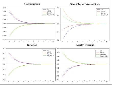
Figure 2: The e¤ects of Loss Aversion.
impulse responses of the variables when the above empirical Taylor rule is im-plemented by setting the weights on in‡ation respectively = 1 and = 2:5, while the weight on output remains the same. In general, by employing the em-pirical rule ‡uctuations are emphasized: in the …rst case as the shock impacts the system the interest rate fall is doubled. As consequence of this, being assets’ returns farther from the reference point, assets’ demand falls about 0.1% and current consumption rises more than 2%. This e¤ect triplicates the in‡ationary response at the impact, while the adjustment process leading to the steady-state comes to be smoothed.
Figure 3: E¤ects of di¤erent monetary policies.
3.3
Changing the Reference Point
The LANK model assumes agents have a state-dependent preference on their …nancial assets’ returns. In the previous paragraphs this preference refers to the displacement of the interest rate from its steady-state value. A natural shortcoming of a de…nition like this is that the reference point does not change at any time. Therefore, an attempt to improve the LANK model is involved by changing the de…nition of the reference point. The simplest way to do this is to assume the reference point as the short term interest rate occurred one-period before, so that function f(z)is rede…ned as follow:
f(Zt) = Bt
Pt (hit it 1) ; Zt 0
Bt
Pt (it it 1)
i
; Zt <0
This new de…nition does not imply any other analytic hurdle in so far as the only di¤erence in respect to the previous de…nition is in the LANK-IS curve:
yt =Et[yt+1]
1
(it Et[ t+1] +rn) +k C (it it 1)
line). As the shock hit the system assets’ demand falls, while consumption and in‡ation rise. However, consumption and assets’ demand impacts are the same as the previous case while the impact on in‡ation is fewer: why this? When the reference point is assumed to be the steady-state interest rate the evaluation of …nancial preference does not change time by time, in the sense that taking the reference point …xed, the size of any displacement from the steady-state of any variable will depend only on the magnitude of the shocks: for a given positive monetary shock the interest rate will be always below the steady-state up to the equilibrium, therefore households always experience a …nancial loss.
On the contrary, when the reference point is updated time by time some changes in agents’ evaluation should a¤ect di¤erently the business cycle. In the present case, households’ reference interest rate changes period-by-period and in particular they take the one occurred one-period-before. When the economy is hit by a positive exogenous shock the interest rate falls and households experience a loss in …nancial gains which increases their consumption and lower their assets’ demand, but when in the next period they look at t 1 interest rate they expe-rience a gain because CB is rising the interest rate. Therefore, from the period after the shock up to the equilibrium will be always it 1 < it, then households
Figure 4: Change in reference point.
4
Conclusions
aversion were able to explain non-trivial evidences such as the equity premium puzzle and the non-partecipation puzzle in the …nancial markets.
Despite the original …eld of application of PT some authors state that PT can be used in a riskless environment also27, and this is the …eld where the LANK
model collocates. Both Kahneman and Tversky and Koszegi and Rabin tried to interpret PT in this sense, assuming individuals derive utility from current consumption relative to some reference level, and that utility function presents both loss aversion and diminishing sensitivity. These studies have paved the way for a new usage of PT in macroeconomics theory: in a Lucas islands’ economy, Ciccarone and Marchetti assumed an utility function accounting for agents’ eval-uation of …nancial wealth that is a¤ected by reference dependence, loss aversion and diminish sensitivity. These assumptions imply agents are worried to su¤er future losses, thus they anticipate the possibility that a monetary shock hits the economy by lowering their labor supply as a form of precautionary behavior. Moreover, due to loss aversion, this engender a sort of attenuation e¤ect on the real variables which reduces output variability. The same precautionary behavior takes place in another contribution of Ciccarone, Marchetti and Giuli where loss aversion agents are assumed in an overlapping generations economy.
Ga¤eo et al. show that loss aversion would be able to explain the asymmetric responses of output and prices to monetary innovations over contractionary and expansionary phases of the business cycle. In the literature this constitutes a rare attempt to insert PT in a standard NK-DSGE. However, even though they face a similar theoretical framework, the LANK model has a di¤erent shape. Indeed, in the LANK model, both narrow framing and loss aversion do not enter in agents’ expectations but in agents’ current decisions.
Section 2 de…nes the peculiarities of the LANK model. The only di¤erence in respect with the baseline NK-DSGE model is in the households’ utility function which presents a component controlling preferences on …nancial wealth. This preference is called narrow framing because agents consider it separately from their other optimal choices (consumption and labor supply) and it enters in the utility function through a parameter that makes the LANK model a portable extension of a standard NK-DSGE. By de…ning the function governing …nancial wealth’s preference two di¤erent optimal conditions for …nancial assets’ demand are obtained. When the current short term interest rate is lower than the steady-state interest rate (reference point) agents reduce their assets’ demand by more than an increase due to an equally sized positive displacement between interest rates. This is the e¤ect of loss aversion which in turn a¤ects the entire dynamic of the system. Therefore, the dynamic of consumptions is described by two Euler equations that change according with the position of the interest rate in respect to the reference point. As consequence of this, the LANK model displays two IS curves that di¤er just for the parameter controlling loss aversion that, therefore, is set equal to one when the interest rate is above the reference point (no loss aversion).
Section 3 analyzes the robustness of the LANK model by hitting the system through exogenous stochastic monetary shocks. The …rst exercise shows that if the coe¢cient controlling …nancial wealth’s preference (k) is set equal to zero, when hit by a positive monetary shock the LANK model performs as a standard NK-DSGE. This con…rm the fact that the LANK model is a portable exten-sion of an existing model (PEEM) that is a key requirement for macroeconomic models presenting behavioral assumptions. As k exceeds zero narrow framing
takes place: for a given positive monetary shock the interest rate goes below the steady-state and households experience a loss in …nancial returns each period. Therefore, narrow framing implies households …nd more convenient to reduce …nancial assets’ demand and to increase current consumption which ‡uctuates more along the business cycle. This is due to the fact that households prefer to consume income they earn rather than to invest in assets because this may imply further losses that they would experience badly.
Anyway, in respect with standard model the short term interest rate responds weakly at the impact because any of its negative variation has a greater e¤ect on both consumption and in‡ation so that CB responds strongly. Moreover, the e¤ect of narrow framing is dampened when the shock changes in the sign: indeed loss aversion implies ‡uctuations of real variables are accentuated when the shock lowers the interest rate. Therefore, equally sized positive and negative monetary shock display asymmetric e¤ects.
In the second exercise the LANK model is tested making di¤erent assump-tions on monetary policy. Also in this case the LANK model performs consis-tently with the predictions: all ‡uctuations are braked when CB weights more in‡ation objective. On the contrary, by employing an empirical Taylor rule ‡uc-tuations are emphasized: in particular the shock implies a doubled fall of the interest rate which in the LANK model implies consistent ‡uctuations in both consumption and in‡ation. In particular, the latter are accentuated because of changes in expectations: agents expect to su¤er more prolonged …nancial losses and then to consume more.
However, taking the steady-state interest rate as reference point prevents the LANK model to describe a reference dynamic. This means that agents do not change their perception of …nancial wealth according to the state of the world they are living. When a positive monetary shock occurs agents always experience a loss until the interest rate reaches the equilibrium. In order to overcome this shortcoming, the LANK model is improved considering the one-period-before interest rate as reference point. When the positive shock occurs agents experience a loss at the impact but gains the periods ahead up to the equilibrium. In the periods next to the shock they have a reference lower than the current interest rate because CB is rising the rate to achieve dynamically the equilibrium. This version of the LANK model moderates the expectation on in‡ation at the impact because the interest rate path has a more smooth pro…le. However the e¤ects on consumption and assets’ demand at the impact are the same.
Summing up, the LANK model accentuates the dynamics of real variables preserving the characteristics of the standard NK-DSGE model. This conclusion seems sharply in contrast with the recent literature introducing Prospect Theory in macroeconomic models. In particular, these models predict that loss aversion engenders an attenuation e¤ect on consumption. Agents are aware that resources they bring in the future may be a¤ected by monetary shocks, thus they reduce labor supply as a sort of precautionary behavior. As a result, the consumption of the next period results lower.
Therefore, the models di¤er due to distinct intertemporal dynamics, but the ef-fects of loss aversion on …nancial assets’ detention are not inconsistent: when bonds are alternative to consumption loss aversion enhances consumption ‡uc-tuations, instead, when bonds are a mean to consume loss aversion negatively a¤ects consumption through a lower labor supply.
The LANK model produces outcomes which are consistent with standard NK-DSGE predictions, it incorporates a state-dependent preference by adding an ad hoc function to the standard utility. Due to simplifying assumptions the model might came under severe criticism, but what has been accurately safe-guarded is that all the envisaged predictions have been successfully ful…lled. It is a belief that there is room to improve the model and …x its shortcomings. Indeed it is recognized that in order to make possible the log-linearization of the system around the steady-state the function governing …nancial preferences does not preserve the curvature28 of the utility function. This would require further
researches providing a di¤erent speci…cation of the utility function. Moreover, a step forward may be to introduce a more versatile de…nition of the reference point’s properties providing a better description of the dynamics, especially mak-ing expectations on future …nancial returns. Bemak-ing all the limitations of the LANK model ‡agged, once they are solved one should test LANK performances in reproducing macroeconomic results. Of course, the LANK model is just a naive attempt to introduce loss aversion in dynamic macroeconomic theories, notwithstanding it may represent a good starting point to consider behavioral hypotheses into a more structured DSGE.
APPENDIX
The Euler equation is rearranged as follow:
1 = RtE(CCt
1+rn. Therefore, denoting with lower-case-letters the percentage deviations of the variables from their steady-state solution, e.g. xt ' XtXX , we obtain:
ct =Et(ct+1) 1
[it Et( t+1) +rn+k C (it rn)]
Model improvements attempt
In order to have decreasing marginal utility we try to change the de…nition of state-dependent preference by exploiting the coe¢cient of intertemporal elasticity of substitution as follow:
The resulting FOC on bonds is
t=
Therefore, the Euler equation takes the following shape:
t
Ct RtCt+1= 8 > < > :
1 "
k(1 ) Bt
Pt
#
| {z }
it
1 "
k(1 ) Bt
Pt
#
| {z }
rn
9 > = > ;
1 1
m m
Ct RtCt+1 =fmit mrng
1 1
Now, trying to linearize just the right-hand-side of the above equation we obtain:
1 1 fmr
n mrng1 mi
trn = 0
References
[1] Barberis, N., Huang, M., 2009. Preferences with frames: A new utility spec-i…cation that allows for the framing of risks. Journal of Economic Dynamics and Control, 33(8), 1555-1576.
[2] Barberis, N., Huang, M., Santos, T., 2001. Prospect theory and asset prices. Quarterly Journal of Economics 116, 1-53.
[3] Barberis, N., Huang, M., Thaler, R.H., 2006. Individual preferences, mon-etary gambles, and stock market participation: a case for narrow framing. American Economic Review 96 (4), 1069–1090.
[4] Benartzi, S. and R.H. Thaler (1995), Myopic loss aversion and the equity Premium puzzle, in: The Quarterly Journal of Economics, vol. 110, no. 1: 73-92.
[5] Blanchard, O., Kiyotaki, N., 1987. Monopolistic competition and the e¤ects of aggregate demand. American Economic Review 77, 647-666.
[6] Ciccarone, G., Giuli, F., Marchetti, E., 2013. Power or loss aversion? Rein-terpreting the bargaining weights in search and matching models. Economics Letters 118, 375-377.
[7] Ciccarone, G., Marchetti, E., 2013. Rational expectations and loss aversion: potential output and welfare implications. Journal of Economic Behavior and Organization 86, 24-36.
[8] Clarida, R., Galí J., Gertler, M., 1999. The science of monetary policy: A new keynesian perspective. Journal of Economic Literature 37, 1661{1707.
[9] De Grauwe P., Lectures on Behavioral Macroeconomics, 2012. Princeton University Press.
[10] Ga¤eo, E., Petrella, I., Pfajfar, D., Santoro, E. (2010). Reference-dependent preferences and the transmission of monetary policy, Center for Economic Studies, Discussions Paper Series (DPS) 10.28.
[11] Galí, J. David Lopez-Salido and Javier Valles. Rule-of-Thumb Consumers And The Design Of Interest Rate Rules, Journal of Money, Credit and Banking, 2004, v36(4,Aug), 739-763.
[12] Galí, J., 2008. Monetary policy, in‡ation, and business cycle. Princeton University Press.
[13] Kahneman, D., Tversky, A., 1979. Prospect theory: an analysis of decisions under risk. Econometrica 47 (2), 263–291.
[14] Kahneman, D., Tversky, A., 1992. Advances in prospect theory: cumulative representation of uncertainty. Journal of Risk and Uncertainty 5 (4), 297– 323.
[16] Keynes J. M., 1936. The general theory of employment, interest and money. London, MacMillan.
[17] Koszegi, B., Rabin, M., 2006. A model of reference-dependent preferences. The Quarterly Journal of Economics 121, 1133-1165.
[18] Mankiw, N.G., 1985. Small menu costs and large business cycles: A macro-economic model. Quarterly Journal of Economics 100, 529-538.
[19] Rabin, M., 2013. An Approach to Incorporating Psychology into Economics. The American Economic Review, Volume 103, Number 3, May 2013, pp. 617-622(6)