Notes from "Monetary Policy, Inflation, and Business Cycle: an Introduction to the New Keynesian Model",
Jordi Galì (2008)
Irina Belousova
1 New Keynesian Model
1.1 Households optimal behaviour
We assume in this model the presence of a retail sector that uses homoge-neous wholesale good to produce a basket of differentiated goods for con-sumption whereǫis the elasticity of substitution. For each i, the consumer chooses Ct(i) at a pricePt(i)to maximize (1) given total expenditure
Z 1
0
Pt(i)Ct(i)di=z (2)
Note, it is assumed the existance of a continuum of goods represented by the interval [0,1].
This optimization problem is solved in the following way
L=
We can now construct the new equation for total expenditure, substitut-ing the latter expression forCt(i)
Z 1
0
Pt(i)Ct(i)di=z
Z 1
0
Pt(i)Ct(j)Pt(j)ǫPt(i)−ǫdi=z
Ct(j)Pt(j)ǫ
Z 1
0
Pt(i)1−ǫdi=z
Ct(j) =
zPt(j)−ǫ
R1
0 Pt(i)1−ǫdi
Ct(j) =
zPt(j)−ǫ
R1
0 Pt(i)1−ǫdi
1 1−ǫ
1−ǫ
finally,
Ct(j) = zPt(j)
−ǫ
Pt1−ǫ (3)
where Pt = hR01Pt(i)1−ǫdi
i 1 1−ǫ
is the aggregate price index. Ct and Pt
are Dixit-Stigliz aggregates, see [2].
Similarly, we have the expression for good i, that is Ct(i) = zPt(i)
−ǫ
Pt1−ǫ Subsitute this expression back into the aggregate consumption index
Ct=
Z 1
0
Ct(i)1−
1 ǫdi
ǫ ǫ−1
= Z 1
0
zPtǫ−1Pt(i)−ǫ
1−1 ǫ di
ǫ ǫ−1
=zPtǫ−1 Z 1
0
Pt(i)1−ǫdi
−ǫ 1−ǫ
=zPtǫ−1 "Z 1
0
Pt(i)1−ǫdi
1 1−ǫ#
−ǫ
=zPtǫ−1Pt−ǫ =zPt−1
therfore, z=CtPt, and the new equation for total expenditure becomes
Z 1
0
Now, substitute for zinto equation (3) Ct(i) =zPtǫ−1Pt(i)−ǫ
=CtPtPtǫ−1Pt(i)−ǫ
=Ct
Pt(i)
Pt
−ǫ
(5) we,thus, end up with the equation of relative demand for the differenti-ated good iwith price Pt(i).
Next, we assume that household maximizes the utility function, given the period budget constraint
max
CtNt E0
X∞
t=0
βtU(Ct, Nt)
s.t. Z 1
0
Pt(i)Ct(i) +QtBt≤Bt−1+WtNt+Tt
Assuming the form of utility function as follows U(CT, Nt) =
Ct1−σ 1−σ −
Nt1+ϕ 1 +ϕ the Lagrangian becomes
L=E0
X∞
t=0
" βt C
1−σ t
1−σ − Nt1+ϕ 1 +ϕ
!
+λt(Bt−1+WtNt+Tt−PtCt−QtBt)
#
The first order conditions with respect to Ct andNt are, respectively
∂L
∂Ct
=UC,t−λtPt= 0
UC,t =λtPt
βtCt−σ =λtPt
and,
∂L
∂Nt
=UN,t+λtWt= 0
−UN,t=λtWt
βtNtϕ =λtWt
hence, marginal rate of substitution between consumption and labour is
−UN,t
UC,t
= λtWt λtPt
βtNtϕ βtC−σ
t
= Wt Pt
Ntϕ Ct−σ =
Wt
Pt
Next, we carry out the Euler equation by deriving the Lagrangian with respect toCt andBt−1. Re-express Lagrangian in the following form
L = E0
X∞
s=0
βt+s C
1−σ t+s
1−σ − Nt1++sϕ 1 +ϕ
! +
+λt+s(Bt+s−1+Wt+sNt+s+Tt+s−Pt+sCt+s−Qt+sBt+s)
The first derivative with respect toCt is
∂L
∂Ct
=UC,t+s−λt+sPt+s= 0
UC,t+s =λt+sPt+s
βt+sCt−+σs =λt+sPt+s
these, for different values ofs, become UC,t=βtCt−σ =λtPt, if s= 0
UC,t+1 =βt+1Ct−+1σ =λt+1Pt+1, if s= 1
Next, the first derivative with respect toBt−1 is
∂L
∂Bt−1
=λt+s−λt+s−1Qt+s−1 = 0
λt+s =λt+s−1Qt+s−1
λt+1=λtQt
where the last equality is true for s= 1. Combiningλt+1 and λt, we obtain
UC,t+1
Pt+1
=λtQt
UC,t+1
Pt+1
= UC,t Pt
Qt
ending up with the Euler equation Qt=Et
UC,t+s
UC,t
Pt
Pt+1
=βEt
Ct+1
Ct
−σ
· Pt
Pt+1
(7) The next step is to log-linearize equations (6) and (7). Start with the first one
Ntϕ Ct−σ =
Wt
Pt
ϕlnNt+σlnCt= lnWt−lnPt
ϕ1
N(Nt−N) +σ 1
C(Ct−C) = 1
W(Wt−W)− 1
P(Pt−P)
Note that, the left and right-hand sides of the equation calculated in the mean values have been omitted, since cancelling each other. The same is true for log-linearization of the Euler equation
Qt=βEt
Ct+1
Ct
−σ
· Pt
Pt+1
lnQt= lnβ−σ(lnCt+1−lnCt) + lnPt−lnPt+1
lnQt= lnβ−σ
1
C(Ct+1−C)− 1
C(Ct−C)
+ 1
P(Pt−P)− 1
P(Pt+1−P) lnQt= lnβ−σct+1+σct+pt−pt+1
σct=σct+1−[−lnQt+ lnβ−(pt+1−pt)]
ct=Et{ct+1} −
1
σ (it−ρ−Et{πt+1}) (9)
where it = −lnQt = ln(1 +yield)−1−1 is the nominal interest rate,
ρ=−lnβis the household’s discount rate, andπt=pt−pt−1 is the inflation
rate.
1.2 Firms optimal behaviour
Before proceedeing, let us list the main assumptions undertaken here: there is a continuum of firms indexed by i ∈ [0,1] ; firms produce differentiated goods; technology, At, is identical for each firm and evolves exogenously
over time; each firm deal with an identical isoelastic demand, given in (5); aggregate price index, Pt, and aggregate consumption index, Ct, are given;
following the formalism proposed in [1], each firm may reset its price only with probability (1−θ) in any given period, while a fraction θ keep their prices unchanged; therefore, we can interpret 1−1θ as the average duration of a price, andθ becomes a natural index of price stickiness.
This setting leads to inflation, that can be formalized as follows: assume S(t)⊂[0,1]be the set of firms that not reoptimize their price, and that all firms resetting price will choose an identical price Pt∗. Then, the aggregate price level can be re-expressed in the followin way
Pt=
Z
S(t)
(Pt−1(i))1−ǫdi+ (1−θ)(Pt∗)1−ǫ
1 1−ǫ
Therefore,
Log-linearizing around the zero inflation steady state, that is P∗
t =
Thus, the equation for inflation becomes:
πt= (1−θ)(p∗t −pt−1) (10)
this results from the fact that, firms reoptimizing each period, choose a price that differs from the economy’s average price of the previous pe-riod. Therefore, a firm reoptimizing in periodt will choose a price Pt∗ that maximizes the current market value of the profits, in light of current and anticipated cost conditions. The optimization problem, given the sequence of demand constraints, is as follows
max the stochastic discount factor for nominal payoffs,Ψt(·)is the cost function,
int.
What follows is the derivation of the first order condition associated with the problem above.
Substitute the constraint into the objective function:
max last reset its price in period t, and M = ǫ−ǫ1 is the desired or frictionless mark-up. Note that, if there are no price rigidities, that isθ = 0, the first order condition collapses to the optimal price-setting condition under flexible prices
Pt∗=Mψt|t
which allows us to interpret Mas the desired mark-up in the absence of constraints on the frequency of price adjustment.
and re-express it as follows firm whose price was last set in periodt.
Note that, in steady state, the following relations hold: Pt∗
Pt−1 = 1 and Πt−1,t+k = 1, moreover, if the price level is constant, Pt∗ =Pt+k in steady
state, from which follows that Yt+k|t = Y and M Ct+k|t =M C, that is, all firms will produce the same level of output. This implys M C = M1 under constancy of price level.
Moreover, recalling the Euler equation in (7), that is Qt,t+k=βkEt
Hence, the first-order Taylor expansion of (12) around the zero inflation steady state is as follows
If we definemc\t+k|t≡mct+k|t+lnM=mct+k|t−mc, as the log deviation of marginal cost from its steady state value, mc =−lnM, then the firm’s price-setting decision can be expressed as
p∗t −pt−1 = (1−βθ)
∞ X
k=0
(βθ)kEt{mc\t+k|t+ (pt+k−pt−1)} (13)
Firms resetting their prices will choose a price that corresponds to the desired mark-up,lnM, over a weighted average of their current and expected nominal marginal costs. The weights are proportional to the probability of the price remaining effective at each horison,θk.
1.3 Market clearing conditions
In the market of goods the condition is that Yt(i) = Ct(i), that is, all the
output must be consumed, for all i ∈ [0,1] and t. This implys that the aggregate output can be expressed as follows
Yt=
Z 1
0
Yt(i)1−
1 ǫdi
ǫ ǫ−1
(14) and that aggregate output equals aggregate consumption,Yt=Ct.
There-fore, it can be written in terms of Euler equation yt=Et{yt+1} − 1
σ (it−Et{πt+1} −ρ) (15)
and of equilibrium equation of relative demand for goods, recalling (5)
Yt(i) =
Pt(i)
Pt
−ǫ
Yt (16)
As to the labour market, clearing condition requires Nt =
R1
0 Nt(i)di.
Assuming a Cobb-Douglas production function, that is
Yt(i) =AtNt(i)1−α (17)
re-express it for Nt(i) and substitute into the clearing condition, as
fol-lows
Nt(i) =
Yt(i)
At
1 1−α
Nt=
Z 1
0
Yt(i)
At
1 1−α
Using the last expression, substitute for Yt(i) from equation (16)
We can now log-linearize this new expression for labour, as shown below
Nt=
we, thus, end up with
(1−α)nt=yt−at+dt
can be ignored, as will be shown right below, so that the log-linearized labour equilibrium condition becomes
(1−α)nt =yt−at
nt=
yt−at
1−α (18) In fact, in the expression fordt,diis a measure of price dispersion across
firms. In a neighborhood of zero inflation steady state dt approaches zero
up to a first order Taylor approximation. The demonstration follows imme-diately. Recall
re-definition of price index
lnPt= lnP. Hence, we calculate all the terms needed for the Taylor
expan-sion
Therefore, the Taylor expansion becomes 1 =
0 lnPt(i)di is the cross-sectional mean of log
Note that
Now, go back to the expression fordtin equation (19), and Taylor-expand
up to the second order the term under the integral Z 1
Note that ln(1 +n)≃n, therefore the last expression becomes dt= (1−α)
from the Cobb-Douglass production function Yt(i) =AtNt(i)1−α
M P Nt=
∂Yt(i)
∂Nt(i)
=At(1−α)Nt(i)−α
lnM P Nt= lnAt+ ln(1−α)−αlnNt(i)
mpnt=at−αnt+ ln(1−α)
Substitute for ntfrom equation (18), so that
mpnt=at−α
yt−at
1−α + ln(1−α) mpnt=
at(1−α)−αyt+αat
1−α + ln(1−α) mpnt=
at−αyt
1−α + ln(1−α) (20) Next, we find the real marginal cost, mct+k|t, in t+k for a firm whose price was last set in t, and substitute it in the equation for price setting decision.
Hence, recall equations (13), (18), and (20). First, note that marginal cost of an individual firm in terms of the economy’s average real marginal cost can be expressed as
mct= (wt−pt)−mpnt
subsituting formpntfrom equation (20), we find
mct= (wt−pt)−
at−αyt
1−α −ln(1−α) (21) The same is done for the marginal cost af a firm whose price was last set in periodt
mct+k|t= (wt+k−pt+k)−mpnt+k|t
= (wt+k−pt+k)−
1
1−α(at+k−αyt+k|t)−ln(1−α)± αyt+k
1−α = (wt+k−pt+k)−
1
1−α(at+k−αyt+k) + α
1−αyt+k|t− α
1−αyt+k−ln(1−α) =mct+k+
α
1−αyt+k|t− α 1−αyt+k =mct+k+
α
Using, the market clearing conditionCt=Yt, define the output as follows
Note that, under the assumption of constant returns to scale, α= 0, we obtainmct+k|t=mct+k, that is, marginal cost is independent of the level of
production and, hence, it is common across firms.
1
Note that, the latter expression can be rewritten as p∗t −pt−1= (1−βθ)
p∗t −pt−1= (1−βθ)
Recall, now, the log linearized expression for inflation given in (10), that is
We can clearly see in the above equation for inflation that it is strictly decreasing in the index of price stickiness θ, in the measure of decreasing returnsα, and in the demand elasticity ǫ.
wherelimk→+∞βk+1Et{πt+k+1}= 0, so that the last term on the
right-hand side of the equation disappears.
We can conclude that inflation will be high when firms expect average markups to be below their steady state (i.e. desired) level (mct = lnM),
for in that case firms that have the opportunity to reset prices will choose a price above the economy’s average price level in order to realign their markup closer to its desired level. Moreover, note that, in this model setting inflation results from the aggregate consequences of price-setting decisions by firms, which adjust their prices in light of current and anticipated cost conditions. Next, we need to derive an expression for real marginal costsmcdt, that
ap-pear in equation of inflation (23). For this purpose, recall the equation of economy’s marginal cost (21), and substitute in it the equation of optimal labour supply (8), as follows
mct=ϕnt+σct−
at−αyt
1−α −ln(1−α)
Hence, use the log-linearized relation between aggregate output, employ-ment and technology (18), and the goods market clearing condition(yt=ct),
to obtain
mct=ϕ
yt−at
1−α +σyt−
at−αyt
1−α −ln(1−α) =
ϕ+α 1−α +σ
yt−
1 +ϕ
1−αat−ln(1−α) (24) that is the average real marginal cost of the economy.
Recalling that under flexible prices the real marginal cost is constant, mc=−lnM, define the natural level of output ytn, as the equilibrium level of output under flexible prices
mc=
ϕ+α 1−α +σ
ytn−1 +ϕ
1−αat−ln(1−α) (25) ynt = 1−α
α+ϕ+ (1−α)σ 1 +ϕ 1−αat−
1−α
α+ϕ+ (1−α)σ[−mc−ln(1−α)] = 1 +ϕ
α+ϕ+ (1−α)σat−
(1−α) [lnM −ln(1−α)] α+ϕ+ (1−α)σ
(26) thus,
ynt =ψyan at+ϑny (27)
whereψn
ya = α+ϕ1++(1ϕ−α)σ and ϑny =−(1−αα)[ln+ϕ+(1M−−ln(1α)σ−α)] >0.
Subtract (25) from (24) d
mct=mct−mc=mct+ lnM=
ϕ+α 1−α +σ
that is, the log deviation of real marginal cost from its steady state is proportional to the log deviation of output from its natural level with flexible prices, named output gap(˜yt≡yt−ynt).
Finally, equation (28) is used to remodel equation (23) πt=
(1−θ)(1−βθ) θ
1−α 1−α+αǫ
ϕ+α 1−α +σ
(yt−ynt) +βEt{πt+1}
or, simply
πt=βEt{πt+1}+ky˜t (29)
wherek= (1−θ)(1θ−βθ)1−1α−+ααǫϕ1−+αα+σThis equation is the New Key-nesian Phillips Curve (NKPC), that relates inflation to its one period ahead forecast and the output gap, and represents one of the key equations of the New Keynesian model. The second key equation is derived by expressing equation (15) in terms of output gap,y˜t, given a path for exogenous natural
rate,rtn, and the actual real rate,it, as follows
yt=Et{yt+1} −
1
σ (it−Et{πt+1} −ρ) yt−ytn=Et{yt+1} −
1
σ (it−Et{πt+1} −ρ)−y
n
t ±Et{ytn+1}
˜
yt= Et{yt+1} −Et{ynt+1}
− 1
σ(it−Et{πt+1} −ρ) + Et{y
n
t+1} −ynt
˜
yt=Et{y˜t+1} −
1
σ (it−Et{πt+1} −ρ) +Et{∆y
n t+1}
˜
yt=Et{y˜t+1} −
1
σ it−Et{πt+1} −ρ−σEt{∆y
n t+1}
The last two terms on the right hand-side of the latter expression can be substituted by the natural rate of interest, rn
t, as is shown below. Recall
the definition of real interest rate as the expected real return on one period bondrt=it−Et{πt+1}, and substitute it in equation (15) to get
yt=Et{yt+1} − 1
σ(rt−ρ) rt=σ(Et{yt+1} −yt) +ρ
=σ(Et{∆yt+1}) +ρ
Similarly, thenatural rate of interest becomes rnt =σ Et{∆ynt+1}
+ρ
Therefore, the expression for output gap becomes ˜
yt=Et{y˜t+1} −
1
σ (it−Et{πt+1} −r
n
t) (31)
The equation above is the Dynamic IS equation, DIS, that determines the output gap given a path for the (exogenous) natural rate and the actual real rate. The forward solution of DIS is
˜
yt=Et{y˜t+1} − 1
σ(it−Et{πt+1} −r
n t)
=
Et{y˜t+2} − 1
σ it+1−Et{πt+2} −r
n t+1
− 1
σ(it−Et{πt+1} −r
n t)
=
Et{y˜t+3} −
1
σ it+2−Et{πt+3} −r
n t+2
+
− 1
σ it+1−Et{πt+2} −r
n t+1
− 1
σ(it−Et{πt+1} −r
n t)
· · ·
˜ yt=−
1 σ
∞ X
k=0
it+k−πt+k+1−rtn+k
+Et{y˜t+k+1}
=−1
σ ∞ X
k=0
rt+k−rtn+k
(32)
where the last equation results from the assumption that the effects of nominal rigidities vanish asymptotically,limk→∞Et{y˜t+k+1}= 0. Equation
(32) shows that output gap is proportional to the sum of current and antic-ipated deviations between the real and the natural real interest rates. Equations (29), (31) and (30) constitute the non-policy block of the basic New Keynesian model.
Having assumed in this model that prices are sticky, the Monetary pol-icy is non-neutral, that is, the equilibrium path of real variables cannot be determined independently of monetary policy. Thus, in order to close the model, we need one or more equations determining how the nominal interest rate,it evolves over time, i.e. how monetary policy is conducted.
1.5 Equilibrium under an Interest Rate Rule
Assume the simple interest rate rule of the form
where ϑt is exogenous and possibly stochastic with Et{ϑt} = 0. And
assume that the monetary authority has the possibility to set the (non-negative) values for both the coefficients φπ, and φy. In order to find the
equilibrium conditions, we must solve the following system of difference equa-tions, using (29), (31) and (33)
// ˜
yt= σ+φπσk+φyEt{y˜t+1}+σ+1φ−πφkπ+βφyEt{πt+1}+[(r
n t−ρ)−ϑt]
σ+φπk+φy
πt= σ+φkσπk+φyEt{y˜t+1}+kσ++βφ(πφky++φσy)Et{πt+1}+ k[(r
n t−ρ)−ϑt]
σ+φπk+φy
We can write the above system in the following way
y˜t
πt
=AT
Et{y˜t+1} Et{πt+1}
+BT [(rtn−ρ)−ϑt] (34)
where
At=
1 σ+φπk+φy
σ 1−βφπ σk k+β(σ+φy)
and
Bt=
1 σ+φπk+φy
1
k
Given that both the output gap and inflation are non-predetermined variables, the system (34) will have a unique local solution, if and only if, matrix At has both eigen values (λy, λπ) within the unit circle. The eigen
values of a matrix are defined byA−λI = 0, whereI is the identity matrix, or, furthermore, by (λy−1)(λπ−1)>0, that is λyλπ−(λy +λπ) + 1>0,
or, similarly, det(A)−trace(A) + 1>0, with λyλπ =det(A) andλy+λπ =
In our case, we have
det(A) = σ[k+β(σ+φy)]−σk(1−βφπ) (σ+φπk+φy)2
= σk+βσ
2+βφ
yσ−σk+βφπσk
(σ+φπk+φy)2
= βσ(σ+φπk+φy) (σ+φπk+φy)2
= βσ σ+φπk+φy
trace(A) = σ+k+βσ+βφy σ+φπk+φy
Therefore,det(A)−trace(A) + 1>0 becomes βσ
σ+φπk+φy
−σ+k+βσ+βφy
σ+φπk+φy
+ 1>0 βσ−σ−k−βσ−βφy+σ+φπk+φy >0
k(φπ −1) +φy(1−β)>0 (35)
Expression (35) is referred to as Taylor Principle and represents a nec-essary and sufficient condition for unique solution.
1.5.1 The effects of a monetary policy shock
We will now analyze the response of economy’s equilibrium to an exogenous monetary policy shock, under the interest rate rule given in (33) . Assume the exogenous component,ϑt, in the interest rate rule follows an AR(1) process
ϑt=ρϑϑt−1+εϑt (36)
where ρϑ ∈ [0,1), and such that, a positive realization of εϑt means a
contractionary monetary policy shock with a consequent rise in the nominal interest rate; similarly, a negative realization of εϑ
t means an expansionary
monetary policy shock with a consequent decline in the nominal interest rate, given inflation and the output gap. We assume that the natural interest rate, rn
t, is not affected by monetary policy, so that we can setrnt −ρ= 0for allt.
And we guess that the solution takes the formy˜t=ψyϑϑt, andπt=ψπϑϑt,
whereψyϑ and ψπϑ are the coefficients to be determined using the method
of undetermined coefficients.
expression forπt in terms of Et{πt+1} and Et{y˜t+1}
tute it into the latter expression
stitute (33) into (31), as follows ˜
In the latter expression substitute (29) for πt, so that
Now, recall the form of the solutions we guessed, that is ˜
yt=ψyϑ ϑt
πt=ψπϑϑt
Forward them one period, and take the expectations, as followsEt{y˜t+1}=
ψyϑ ϑt+1, and Et{πt+1} =ψπϑϑt+1. In the same manner, forward one
pe-riod equation (36), that becomesϑt+1 =ρϑϑt, beingEt{εϑt}= 0. Therefore,
we end up with
Et{y˜t+1}=ψyϑρϑϑt
Et{πt+1}=ψπϑ ρϑϑt
Use these four expressions into equations (37) and (38). The first one becomes and the latter becomes
ψyϑϑt=
[σ+kφπ+φy−ρϑ(βσ+k+βφy)] (σ+φy +kφπ−σρϑ)−kσρ2ϑ(1−βφπ)
[σ+kφπ+φy−ρϑ(βσ+k+βφy)] (σ+φy+kφπ−σρϑ)
ψπϑ=
= −kσρϑ−k(σ+φy+kφπ−σρϑ)
[σ+kφπ+φy−ρϑ(βσ+k+βφy)] (σ+φy+kφπ −σρϑ)
Cancel out denominators and develope the multiplications
(σ2+φyσ+kφπσ−ρϑσ2+kφπσ+kφπφy +k2φ2π−kφπρϑσ+φyσ+φ2y+kφπφy−φyρϑσ+
−βρϑσ2−βφyρϑσ−βσρϑφπk+βσ2ρ2ϑ−kρϑσ−kρϑφy−k2ρϑφπ+kρ2ϑσ−βφyρϑσ−βφ2yρϑ+
−βφyρϑφπk+βφyρ2ϑσ−σkρ2ϑ+σkρϑ2βφπ)ψπϑ =−kσρϑ−kσ−kφy−k2φπ+kσρϑ
Cancel out ±kρ2ϑσ on the left hand-side of the equality, and ±kσρϑ on
the right hand one.
(σ2+σφy+σφπk−σ2ρϑ+σkφπ+φykφπ +k2φ2π−kφπσρϑ+φyσ+φy2+φyφπk−φyσρϑ+
−βσ2ρϑ−βσφyρϑ−βσρϑφπk+βσ2ρ2ϑ−kρϑσ−kρϑφy−k2ρϑφπ−βφyρϑσ−βφ2yρϑ+
−βφyρϑφπk+βφyρ2ϑσ+σkρ2ϑβφπ)ψπϑ =−k(σ+φy+kφπ)
Now, collect the terms on the left hand-side of the equality
[σ2+φ2y+k2φ2π + 2σφy+ 2σφπk+ 2φyφπk+σ(−σρϑ) +φπk(−σρϑ) +φy(−σρϑ)+
+σ(βσρ2ϑ) +φπk(βσρ2ϑ) +φy(βσρ2ϑ) +σ(−kρϑ) +φπk(−kρϑ) +φy(−kρϑ) +σ(−βφyρϑ)+
φπk(−βφyρϑ) +φy(−βφyρϑ) +σ(−βσρϑ) +φπk(−βσρϑ) +φy(−βσρϑ)]ψπϑ =−k(σ+φy+kφπ)
[(σ+φy+kφπ)2−σρϑ(σ+φπk+φy) +βσρ2ϑ(σ+φπk+φy)−kρϑ(σ+φπk+φy)+
−βφyρϑ(σ+φπk+φy)−βσρϑ(σ+φπk+φy)]ψπϑ =−k(σ+φy +kφπ)
(σ+φy+kφπ)[σ+φy+kφπ−σρϑ+βσρ2ϑ−kρϑ−βφyρϑ−βσρϑ]ψπϑ =−k(σ+φy+kφπ)
[σ(1−βρϑ)−σρϑ(1−βρϑ) +φy(1−βρϑ) +k(φπ−ρϑ)]ψπϑ=−k
{(1−βρϑ) [σ(1−ρϑ) +φy] +k(φπ−ρϑ)}ψπϑ =−k
ψπϑ =
−k
(1−βρϑ) [σ(1−ρϑ) +φy] +k(φπ−ρϑ)
Therefore, πt=
−k
(1−βρϑ) [σ(1−ρϑ) +φy] +k(φπ −ρϑ)
Next, determine the coefficient for output gap. Substituteψπϑ into (40)
ψyϑ =
ρϑ(1−βφπ)
σ+φy+kφπ−σρϑ
· −k
(1−βρϑ) [σ(1−ρϑ) +φy] +k(φπ−ρϑ)
− 1
σ+φy+kφπ−σρϑ
= −kρϑ+kβφπρϑ−[σ+φy+kφπ−σρϑ+βσρ
2
ϑ−kρϑ−βφyρϑ−βσρϑ]
(σ+φy+kφπ−σρϑ){(1−βρϑ) [σ(1−ρϑ) +φy] +k(φπ−ρϑ)}
= σ(−1) +φy(−1) +kφπ(−1)−σρϑ(−1) +σ(βρϑ) +φy(βρϑ) +kφπ(βρϑ)−σρϑ(βρϑ) (σ+φy+kφπ−σρϑ){(1−βρϑ) [σ(1−ρϑ) +φy] +k(φπ−ρϑ)}
= (σ+φy+kφπ−σρϑ)(βρϑ−1)
(σ+φy+kφπ−σρϑ){(1−βρϑ) [σ(1−ρϑ) +φy] +k(φπ−ρϑ)}
ψyϑ =−
1−βρϑ
(1−βρϑ) [σ(1−ρϑ) +φy] +k(φπ−ρϑ)
The response of output gap becomes ˜
yt=−
1−βρϑ
(1−βρϑ) [σ(1−ρϑ) +φy] +k(φπ−ρϑ)
ϑt (42)
As long as Taylor principle is satisfied, (35), denominators of both the coefficients, ψπϑ, ψyϑ, are strictly greater than zero. Hence, an exogenous
increase in the interest rate (εϑt > 0), leads to a persistant decline in the output gap and inflation. Because the natural level of output, see equation (27), is not affected by the monetary policy shock, the response of output maches that of the output gap, y˜t≡yt−ytn≡yt.
Now we want to derive the deviation of real interest rate from its steady state value, that isˆrt=rt−rnt. Replacert=it−Et{πt+1}, and the guessed
solutions for y˜tand Et{y˜t+1} in equation (31)
˜
yt=Et{y˜t+1} −
1
σ(rt−r
n t)
(rt−rnt) =σ(Et{y˜t+1} −y˜t)
ˆ
rt=σ(ψyϑρϑϑt−ψyϑϑt)
ˆ
rt=σ(ρϑ−1)ψyϑϑt
ˆ rt=
σ(1−ρϑ)(1−βρϑ)
(1−βρϑ) [σ(1−ρϑ) +φy] +k(φπ −ρϑ)
ϑt (43)
Equation (43) shows that the deviation of real inrìterest rate from its steady state value increases in response to an exogenous increase in the nominal interest rate (εvt >0 implysϑt>0, which induceit to increase).
and the variation induced by lower output gap and inflation, as shown below ˆit= ˆrt+Et{πt+1}= ˆrt+ψπϑρϑϑt
ˆit= σ(1−ρϑ)(1−βρϑ)−kρϑ
(1−βρϑ) [σ(1−ρϑ) +φy] +k(φπ−ρϑ)
ϑt (44)
If the persistance of monetary policy shock, ρϑ, is sufficiently high, the
nominal rate will decrease in response to a rise in ϑt. This is because the
indirect effect of a positive realization of εϑ
t, that is the decline in inflation
and output gap, more than offset the direct effect of higherϑt, resulting in
a downward adjustment in the nominal rate. In that case, and despite the lower nominal rate, the policy (positive) shock still has contractionary effect on output, because the latter is inversely related to the real rate, which goes up unambiguously.
Assume a log-linear money demand equation of the form
mt−pt=yt−ηit (45)
where η is the interest semi-elasticity of money demand. The response ofmtto change in interest rate, using (41), (42) and (44), is
dmt
dεϑt = dpt
dεϑt + dyt
dεϑt −η dit
dεϑt
= −k−(1−βρϑ)−η[σ(1−ρϑ)(1−βρϑ)−kρϑ] (1−βρϑ) [σ(1−ρϑ) +φy] +k(φπ−ρϑ)
=−(1−βρϑ)[1 +ησ(1−ρϑ)] +k(1−ηρϑ)
(1−βρϑ) [σ(1−ρϑ) +φy] +k(φπ−ρϑ)
(46) Hence, The sign of the change in the money supply that supports the exogenous policy intervention is ambiguous. Note that dit/dεϑt > 0 is a
Appendix 1: Derivation of log-linear money demand equation
Assume the following utility function
U(Ct,Mt
Pt
, Nt) = C
1−σ t
1−σ +
(Mt/Pt)1−ϑ
1−ϑ − Nt1+φ
1 +φ (47) and a sequence of flow budget constraints
PtCt+QtBt+Mt≤Bt−1+Mt−1+WtNt+Tt
CallAt=Bt−1+Mt−1total financial wealth. Budget constraint becomes
PtCt+QtBt+Mt+QtMt−QtMt≤Bt−1+Mt−1+WtNt+Tt
PtCt+QtAt+ (1−Qt)Mt≤At−1+WtNt+Tt (48)
We want to maximize (47) with respect to consumptionCtand nominal
money demandMt, subject to (48). Hence, the Lagrangian is
L= C
1−σ t
1−σ+
(Mt/Pt)1−ϑ
1−ϑ − Nt1+φ
1 +φ+λ[At−1+WtNt+Tt−PtCt−QtAt−(1−Qt)Mt]
∂L
∂Ct
=UC,t−λPt=Ct−σ−λPt= 0
∂L
∂Mt
=UM,t−λ(1−Qt) =
Mt
Pt
−ϑ
1 Pt
−λPt= 0
The marginal rate of substitution between nominal money demand and consumtion is
UM,t
UC,t
= λPt λ(1−Qt)
Mt
Pt −ϑ
1
Pt Ct−σ =
Pt
1−Qt
So, the demand for real balances becomes Mt
Pt
=Ct−σ(1−Qt)−
1
ϑ =Cσ/ϑ
t (1−exp{−it})−1/ϑ (49)
of (49) is as follows lnMt−lnPt=
σ
ϑlnCt− 1
ϑln(1−exp{−it}) 1
M∗(Mt−M
∗)− 1
P∗(Pt−P ∗) = σ
ϑ 1
C∗(Ct−C ∗)− 1
ϑ
exp{−it}
1−exp{−it}
it
Note that exp{−it}
1−exp{−it}
= 1 exp{it}
:
1− 1
exp{it}
= 1 exp{it}
· exp{it}
exp{it} −1
=
= 1 exp{it} −1
≡ 1
i∗ So, the log-linearization becomes
mt−pt=
σ ϑct−
1 ϑ·
1 i∗it mt−pt=
σ
ϑct−ηit (50)
where ϑi1∗ = ϑ(exp{1i
t}−1) = η is the implied interest semi-elasticity of money demand. In the particular case ofϑ=σ, that implies a unit elasticity with respect to consumtion, a conventional linear demand for real balances becomes
mt−pt=ct−ηit
=yt−ηit (51)
where the latter equality uses the market clearing conditionCt=Yt, that
is all output is consumed.
1.5.2 The effects of a technology shock
Assume an AR(1) process for the technology parameter at
at=ρaat−1+εat (52)
whereρa∈[0,1]and εat is a zero mean white noise process. Note that,
at−at−1 =ρaat−1−at−1+εat
∆at= (ρa−1)at−1+εat
Et{∆at+1}= (ρa−1)at
Given (30), the implied natural rate expressed in terms of deviations from steady state (ˆrn
t =rnt −ρ), is given by
rnt =σψyanEt{∆at+1}+ρ
rnt −ρ=σψyan (ρa−1)at
ˆ
rnt =−σψnya(1−ρa)at (53)
In this case we set ϑt = 0, for all t, that is we turn off the monetary
shocks, and we guess that output gap and inflation are proportional to rˆn t.
The guessed solutions will take the following form ˜
yt=ψyrrˆtn
πt=ψπrrˆnt
and
Et{y˜t+1}=ρaψyrrˆtn
Et{πt+1}=ρaψπrrˆnt
Use the method of undetermined coefficients to find the solutions. Recall the two equations from the system (34)
˜ yt=
σ σ+φy+kφπ
Et{y˜t+1}+
1−βφπ
σ+φy+kφπ
Et{πt+1}+
[(rn
t −ρ)−ϑt]
σ+φy+kφπ
πt=
βσ+k+βφy
σ+kφπ+φy
Et{πt+1}+
kσ σ+kφπ+φy
Et{y˜t+1}+
k[(rtn−ρ)−ϑt]
(σ2+σφy+σkφπ−σ2ρa+kφπσ+kφπφy+k2φ2π−kφπσρa+φyσ+φ2y+kφπφy−φyσρa+
−βσ2ρa−φyβσρa−kφπβσρa+βσ2ρ2a−kρaσ−kρaφy−k2ρaφπ +kρ2aσ−βφyρaσ−βφ2yρa+
−βφyρakφπ+βφyρ2aσ−kσρa2+kσρ2aβφπ)ψπr =k(σ+φy+kφπ)
σ2+k2φ2π+φy2+ 2σφy+ 2σkφπ+ 2kφπφy+σ(−σρa) +kφπ(−σρa) +φy(−σρa) +σ(−βσρa)+
+φy(−βσρa) +kφπ(−βσρa) +σ(−kρa) +φy(−kρa) +kφπ(−kρa) +σ(βσρ2a) +φy(βσρ2a)+
+ [kφπ(βσρ2a) +σ(−βφyρa) +φy(−βφyρa) +kφπ(−βφyρa)]ψπr =k(σ+φy+kφπ)
[(σ+kφπ+φy)2−σρa(σ+kφπ +φy)−βσρa(σ+kφπ+φy)−kρa(σ+kφπ+φy)+
+βσρ2a(σ+kφπ+φy)−βφyρa(σ+kφπ+φy)]ψπr =k(σ+φy+kφπ)
(σ+φy+kφπ)[(σ+φy +kφπ)−σρa−βσρa−kρa+βσρ2a−βφyρa]ψπr =k(σ+φy+kφπ)
[βρa(−σ+σρa−φy) +k(φπ−ρa) +σ(1−ρa) +φy]ψπr =k
{−βρa[σ(1−ρa) +φy] +k(φπ−ρa) +σ(1−ρa) +φy}ψπr =k
ψπr =
k
Continuing withψyr, it becomes
ψyr =
(1−βφπ)ρa
σ+φy+kφπ −σρa
· k
(1−βρa)[σ(1−ρa) +φy] +k(φπ −ρa)
+ 1
σ+φy+kφπ−σρa
= (1−βφπ)ρak+ (1−βρa)[σ(1−ρa) +φy] +k(φπ−ρa) (σ+φy+kφπ−σρa){(1−βρa)[σ(1−ρa) +φy] +k(φπ−ρa)}
= ρak−βφπρak+σ+φy+kφπ−σρa−βσρa−kρa+βσρ
2
a−βφyρa
(σ+φy+kφπ−σρa){(1−βρa)[σ(1−ρa) +φy] +k(φπ−ρa)}
= φπk(1−βρa) +φy(1−βρa)−σρa(1−βρa) +σ(1−βρa) (σ+φy+kφπ−σρa){(1−βρa)[σ(1−ρa) +φy] +k(φπ−ρa)}
= (1−βρa)(σ+φy+kφπ−σρa)
(σ+φy+kφπ−σρa){(1−βρa)[σ(1−ρa) +φy] +k(φπ−ρa)}
ψyr =
1−βρa
(1−βρa)[σ(1−ρa) +φy] +k(φπ−ρa)
Note that, these coefficients are the same as in case of a monetary policy shock (ˆrn
t = 0), but with opposite sign. This, in fact, can be seen from the
system (34), where ϑt and rˆtn enter both the equations for πt and y˜t with
the opposite sign in case of monetary policy shock and technology shock, respectively. Denominator of bothψyr andψπr is strictly greater than zero.
The guessed solutions for inflation and output gap are, respectively πt=ψπrrˆnt =
k
(1−βρa)[σ(1−ρa) +φy] +k(φπ−ρa)
ˆ rnt
=− σψ
n
ya(1−ρa)k
(1−βρa)[σ(1−ρa) +φy] +k(φπ−ρa)
at (54)
˜
yt=ψyrˆrtn=
1−βρa
(1−βρa)[σ(1−ρa) +φy] +k(φπ−ρa)
ˆ rnt
=− σψ
n
ya(1−ρa)(1−βρa)
(1−βρa)[σ(1−ρa) +φy] +k(φπ−ρa)
at (55)
As long as ρa < 1, a positive technology shock (εat > 0) leads to a
persistant decline both in inflation and the output gap. In this case, the natural level of output will be affected by technology shock, see equation (27). The implied equilibrium response of output is given by
yt=ytn+ ˜yt=ψnyaat+ϑny −
σψn
ya(1−ρa)(1−βρa)
(1−βρa)[σ(1−ρa) +φy] +k(φπ−ρa)
at
=ψyan
1− σ(1−ρa)(1−βρa)
(1−βρa)[σ(1−ρa) +φy] +k(φπ−ρa)
And the equilibrium response of employment, starting from equation (18), is
(1−α)nt=yt−at
=ψyan
1− σ(1−ρa)(1−βρa)
(1−βρa)[σ(1−ρa) +φy] +k(φπ−ρa)
at−at
=
(ψyan −1)−ψnya σ(1−ρa)(1−βρa)
(1−βρa)[σ(1−ρa) +φy] +k(φπ−ρa)
at
(57) The sign of the response of output and employment to a positive tech-nology shock is in general ambiguous, depending on the configuration of parameter values.
1.6 Matlab Codes
What follows are some possible codes configuration in Matlab of the model described above. The same calibration of parameters as in the book of Jordi Galì is used.
Therefore, the coding of linearized model in case of an exogenous shock on monetary policy can be written as follows
Matlab Code for Policy Monetary Shock in the NK model with a Taylor Rule
/////////////////////////////////////////////////// //DECLARATION OF ENDOGENOUS VARIABLES// //////////////////////////////////////////////////
var pi y_tilde i v mr y rn y_n a r;
///////////////////////////////////////////////// //DECLARATION OF EXOGENOUS VARIABLES// ////////////////////////////////////////////////
varexo varepsilon_v varepsilon_a;
////////////////////////////////////// //DECLARATION OF PARAMETERS// /////////////////////////////////////
parameters betta sigma varphi alpha varepsilon eta theta phi_pi phi_y rho_v rho_a k lambda THETA psi_yan rho lambda_v; /////////////////////////////////////
betta=0.99; //implies a steady state real return on financial as-sests of about 4%.
sigma=1; //implies a log utility.
varphi=1; //implies a unitary Frisch elasticity of labour supply. alpha=1/3;
varepsilon=6; eta=4;
theta=2/3; //implies an average price duration of three quarters. phi_pi=1.5;
phi_y=0.5/4;
rho_v=0.5; //implies a moderately persistent shock. rho_a=0.9;
THETA= (1−alpha)/(1−alpha+alpha·varepsilon); lambda= (((1−theta)·(1−betta·theta))/theta)·THETA; k=lambda·(sigma+ ((varphi+alpha)/(1−alpha)));
psi_yan= (1 +varphi)/(sigma·(1−alpha) +varphi+alpha); rho=-log(betta);
lambda_a= 1/((1−betta·rho_a)·(sigma·(1−rho_a)+phi_y)+ k·(phi_pi−rho_a));
lambda_v= 1/((1−betta·rho_v)·(sigma·(1−rho_v)+phi_y)+ k·(phi_pi−rho_v));
///////////////////////// //DSGE-Model-equations// ////////////////////////
model(linear);
//New Keynesian Phillips Curve eq. 29. pi=betta·pi(+1) +k·y_tilde;
//Dynamic IS eq. 31.
y_tilde=y_tilde(+1)−(1/sigma)·(i−pi(+1)−rn); //Output Gap.
y_n=y-y_tilde;
//Natural Output eq. 27. y_n=psi_yan·a;
//Natural Rate of Interest eq. 30. rn=rho+sigma·(y_n(+1)−y_n); //Taylor Interest Rate Rule eq. 33.
//Real Interest Rate r=i-pi(+1);
//or, similarly
// r=sigma·(y(+1)−y) +rho; //Real Money Demand eq. 45. mr=y−eta·i;//where mr=m-p,
//AR(1) for monetary policy shock eq. 36. v=rho_v·v(−1) +varepsilon_v;
//AR(1) for technology shock eq. 52. a=rho_a·a(−1) +varepsilon_a;
end;
//////////////////////////// //SHOCK SPECIFICATION// ////////////////////////////
shocks;
var varepsilon_v; stderr 0.25;
var varepsilon_a; stderr 0;
end;
steady;
check;
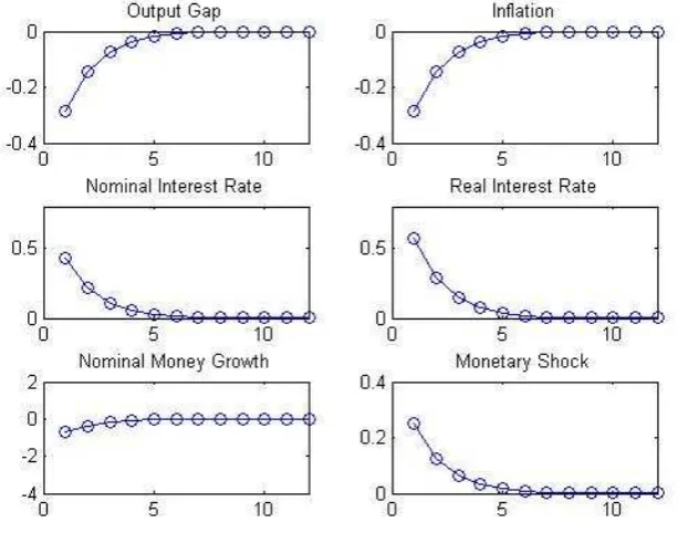
stoch_simul(order=1, irf=12)y_tilde pi i r mr v;
figure(’Name’,’Effects of a Monetary Policy Shock’,’NumberTitle’,’off’);
subplot(3,2,1);
plot(y_tilde_varepsilon_v, ’-o’);
title(’Output Gap’);
axis([0,12,-0.4,0]);
subplot(3,2,2);
plot(4·pi_varepsilon_v,′−o′);
title(’Inflation’);
axis([0,12,-0.4,0]);
subplot(3,2,3);
title(’Nominal Interest Rate’);
axis([0,12,0,0.8]);
subplot(3,2,4);
plot(4·r_varepsilon_v,′−o′);
title(’Real Interest Rate’);
axis([0,12,0,0.8]);
subplot(3,2,5);
plot(mr_varepsilon_v, ’-o’);
title(’Nominal Money Growth’);
axis([0,12,-4,2]);
subplot(3,2,6);
plot(v_varepsilon_v, ’-o’);
title(’Monetary Shock’);
axis([0,12,0,0.4]);
The impulse Response Functions of the variables of interest are (compare these with Figure 3.1 from the book of Galì).
First of all, note that the responses for inflation and the two interest rates are expressed in annual terms. For this purpose their IRFs have been multiplied by 4.
Figure 1, hence, illustrates the dynamic effects of an expansionary monetary policy shock, which corresponds to an increase in εvt of 0.25. In the absence of a further change induced by the response of inflation or the output gap, this would imply an increase of 100 basis points in the annualized nominal interest rate.
The policy shock generates a decrease both in output gap, which effectively corresponds to output, because the natural level of output is not affected by monetary policy shock, and in inflation, and an increase in the real rate. The nominal interest rate increases, too, but by less than its exogenous com-ponent because of a downward adjustment induced by the decline in output gap and inflation. Moreover, the response of the real interest rate is larger than that of the nominal rate due to a decrease in expected inflation. Finally, the model displays aliquidity effect resulting form the actions taken by the Central Bank, which must implement a reduction in money supply given the observed interest rate response.
Matlab Code for Technology Shock in the NK model with a Taylor Rule
/////////////////////////////////////////////////// //DECLARATION OF ENDOGENOUS VARIABLES// //////////////////////////////////////////////////
var pi y_tilde i v mr y rn y_n a r n;
///////////////////////////////////////////////// //DECLARATION OF EXOGENOUS VARIABLES// ////////////////////////////////////////////////
varexo varepsilon_v varepsilon_a;
////////////////////////////////////// //DECLARATION OF PARAMETERS// /////////////////////////////////////
parameters betta sigma varphi alpha varepsilon eta theta phi_pi phi_y rho_v rho_a k lambda THETA psi_yan rho lambda_v; /////////////////////////////////////
//CALIBRATION OF PARAMETERS// /////////////////////////////////////
betta=0.99; //implies a steady state real return on financial as-sests of about 4%.
varphi=1; //implies a unitary Frisch elasticity of labour supply. alpha=1/3;
varepsilon=6; eta=4;
theta=2/3; //implies an average price duration of three quarters. phi_pi=1.5;
phi_y=0.5/4;
rho_v=0.5; //implies a moderately persistent shock. rho_a=0.9;
THETA= (1−alpha)/(1−alpha+alpha·varepsilon); lambda= (((1−theta)·(1−betta·theta))/theta)·THETA; k=lambda·(sigma+ ((varphi+alpha)/(1−alpha)));
psi_yan= (1 +varphi)/(sigma·(1−alpha) +varphi+alpha); rho=-log(betta);
lambda_a= 1/((1−betta·rho_a)·(sigma·(1−rho_a)+phi_y)+ k·(phi_pi−rho_a));
lambda_v= 1/((1−betta·rho_v)·(sigma·(1−rho_v)+phi_y)+ k·(phi_pi−rho_v));
///////////////////////// //DSGE-Model-equations// ////////////////////////
model(linear);
//New Keynesian Phillips Curve eq. 29. pi=betta·pi(+1) +k·y_tilde;
//Dynamic IS eq. 31.
y_tilde=y_tilde(+1)−(1/sigma)·(i−pi(+1)−rn); //Output Gap.
y_n=y-y_tilde;
//Natural Output eq. 27. y_n=psi_yan·a;
//Natural Rate of Interest eq. 30. rn=rho+sigma·psi_yan·(a(+1)−a); //Taylor Interest Rate Rule eq. 33.
i=rho+phi_pi·pi+phi_y·y_tilde+v; //Real Interest Rate
//or, similarly
// r=sigma·(y(+1)−y) +rho; //Real Money Demand eq. 45. mr=y−eta·i;//where mr=m-p,
//Economic Equilibrium Employment eq. 18. n= (1/(1−alpha))·(y−a);
//AR(1) for monetary policy shock eq. 36. v=rho_v·v(−1) +varepsilon_v;
//AR(1) for technology shock eq. 52. a=rho_a·a(−1) +varepsilon_a;
end;
//////////////////////////// //SHOCK SPECIFICATION// ////////////////////////////
shocks;
var varepsilon_v; stderr 0;
var varepsilon_a; stderr 1;
end;
steady;
check;
stoch_simul(order=1, irf=12)y_tilde pi y n i r mr a;
figure(’Name’,’Effects of a Technology Shock’,’NumberTitle’,’off’);
subplot(4,2,1);
plot(y_tilde_varepsilon_a, ’-o’);
title(’Output Gap’);
axis([0,12,-0.2,0]);
subplot(4,2,2);
plot(4·pi_varepsilon_a,′−o′);
title(’Inflation’);
axis([0,12,-1,0]);
subplot(4,2,3);
title(’Output’);
axis([0,12,0,1]);
subplot(4,2,4);
plot(n_varepsilon_a,′−o′);
title(’Employment’);
axis([0,12,-0.2,0]);
subplot(4,2,5);
plot(4·i_varepsilon_a,′−o′);
title(’Nominal Interest Rate’);
axis([0,12,-1,0]);
subplot(4,2,6);
plot(4·r_varepsilon_a,′−o′);
title(’Real Interest Rate’);
axis([0,12,-0.4,0]);
subplot(4,2,7);
plot(mr_varepsilon_a, ’-o’);
title(’Nominal Money Growth’);
axis([0,12,-10,10]);
subplot(4,2,8);
plot(a_varepsilon_a, ’-o’);
title(’Technology Shock’);
axis([0,12,0,1]);
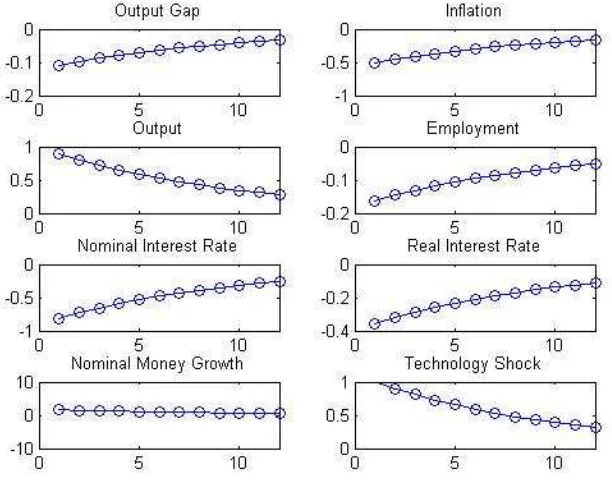
The impulse Response Functions of the variables of interest are illus-trated in Figure 2 (compare these with Figure 3.2 from the book of Galì).
It shows that a positive technology shock leads to a persistent decline in both inflation and output gap. Instead, the responses of output and employ-ment to a positive technology shock are, in general, ambiguous, depending on the calibration of the parameters values.
Given the calibration adopted here, a technological improvement leads to a persistent employment decline, while actual output increses, though less than its natural counterpart.
Fig. 2: Effects of a Technology Shock with Interest Rate Rule
1.7 Equilibrium under an Exogenous Money Supply
The equilibrium dynamics of the basic New Keynesian model is, now, ana-lyzed under an exogenous path for the growth rate of money supply, ∆mt.
Rewrite the money market equilibrium condition (45) in terms of output gap(˜yt=yt−ytn), as follwos
mt−pt=yt−ηit
mt−pt= ˜yt+ynt −ηit
˜
yt−ηit= (mt−pt)−ytn (58)
it=
1
η[˜yt−(mt−pt) +y
n
t] (59)
Substitute equation (59) in the dynamic IS equation (31) ˜
yt=Et{y˜t+1} −1
σ(it−Et{πt+1} −r
n t)
σy˜t=σEt{y˜t+1} −
1
η [˜yt−(mt−pt) +y
n
t] +Et{πt+1}+rtn
that is a difference equation for output gap. In order to complete the system and to find the equilibrium solutions, we need two more equations. The one is the NKPC described in equation (29), the other is an expression for real balances (mt−pt) in relation with inflation and money growth, as
shown below
The log-linearization of this identity becomes
lnMt−lnMt−1 = (lnMt−lnPt)−(lnMt−1−lnPt−1) + (lnPt−lnPt−1)
mt−mt−1 = (mt−pt)−(mt−1−pt−1) + (pt−pt−1)
∆mt= (mt−pt)−(mt−1−pt−1) +πt (61)
Therefore, the three equations that form the system are
The system to be solved is
will exist and be unique, if and only if, matrix
(1 +−kησ) 01 00 0 −1 1
−1
×
ησ η0 β 10 0 0 1
has one eigenvalue outside (or on) the unit circle, and two eigenvalues inside the unit circle. It can be shown, that this condition is always satis-fied, so the equilibrium is always determined under an exogenous path for the money supply (in contrast with the interest rate rule, where the Taylor Principle must hold).
1.7.1 The effects of a monetary policy shock
We want here to analyze the responses of the economy to an exogenous monetary policy shock to the money supply. Assume, for this purpose, an AR(1) process for the growth of money
∆mt=ρm∆mt−1+εmt (63)
whereρm ∈[0,1), andεmt is a zero mean white noise process. A positive
realization of εmt implies an expansionary monetary policy shock. Combine equation (63) with the dynamic system (62)
(1 +ησ) ˜yt=ησEt{y˜t+1}+ηEt{πt+1}+ (mt−pt) +ηrtn−ytn
−ky˜t+πt=βEt{πt+1}
πt+ (mt−1−pt−1) = (mt−pt)−∆mt
∆mt=ρm∆mt−1+εmt
and guess that the solutions will take the following form ˜
yt=ψym∆mt
πt=ψπm∆mt
(mt−1−pt−1) =ψlm∆mt
Forward one period, the AR(1) process for money growth becomes Et{∆mt+1}=ρm∆mt
Therefore, forward one period, the guessed solutions are Et{y˜t+1}=ψymEt{∆mt+1}=ψymρm∆mt
Et{πt+1}=ψπmEt{∆mt+1}=ψπmρm∆mt
Using the method of undetermined coefficients one can find the response functions for output gap, inflation, nominal and real rates, and real balances. Note that in this framework it must be setrˆnt =ytn= 0, for all t.
1.7.2 The effects of a technology shock
Assume once again the technology parameterat follows the stationary
pro-cess given in (52). Combining this with equations (27) and (30) a path is determined forrˆtnandynt as function ofat, which is then used to solve system
References
[1] Guillermo A. Calvo: "Staggered prices in a utility-maximizing frame-work". Volume 12, Issue 3, Journal of Monetary Economics, 1983. [2] Avinash K. Dixit, Joseph E. Stiglitz: "Monopolistic Competition and