Volume5,Issue1 2005 Article13
The 3-Equation New Keynesian Model — A
Graphical Exposition
Wendy Carlin
∗David Soskice
†∗University College London, [email protected] †Duke University, [email protected]
Copyright c2005 by the authors. All rights reserved. No part of this publication may be reproduced, stored in a retrieval system, or transmitted, in any form or by any means, elec-tronic, mechanical, photocopying, recording, or otherwise, without the prior written permis-sion of the publisher, bepress, which has been given certain exclusive rights by the author.
Contributions to Macroeconomics is produced by The Berkeley Electronic Press (bepress).
Graphical Exposition
∗
Wendy Carlin and David Soskice
Abstract
We develop a graphical 3-equation New Keynesian model for macroeconomic analysis to replace the traditional IS-LM-AS model. The new graphical IS-PC-MR model is a simple version of the one commonly used by central banks and captures the forward-looking thinking engaged in by the policy maker. Within a common framework, we compare our model to other monetary-rule based models that are used for teaching and policy analysis. We show that the differences among the models centre on whether the central bank optimizes and on the lag structure in the IS and Phillips curve equations. We highlight the analytical and pedagogical advantages of our preferred model. The model can be used to analyze the consequences of a wide range of macroeconomic shocks, to identify the structural determinants of the coefficients of a Taylor type interest rate rule, and to explain the origin and size of inflation bias.
KEYWORDS:New Keynesian macroeconomics, monetary policy rule, Taylor rule, 3-equation
model, inflation bias, time inconsistency
∗We are grateful for the advice and comments of Christopher Allsopp, James Cloyne, John Driffill,
1
Introduction
Much of modern macroeconomics is inaccessible to undergraduates and to non-specialists. There is a gulf between the simple models found in principles and in-termediate macro textbooks — notably, the IS-LM-AS approach — and the models currently at the heart of the debates in monetary macroeconomics in academic and central bank circles that are taught in graduate courses. Our aim is to show how this divide can be bridged.
Modern monetary macroeconomics is based on what is increasingly known as the 3-equation New Keynesian model:IScurve, Phillips curve and a monetary pol-icy rule equation. This is the basic analytical structure of Michael Woodford’s book Interest and Prices published in 2003 and, for example, of the widely cited paper ‘The New Keynesian Science of Monetary Policy’ by Clarida et al. (1999). An ear-lier in uential paper is Goodfriend and King (1997). These authors are concerned to show how the equations can be derived from explicit optimizing behaviour on the part of the individual agents in the economy in the presence of some nominal imperfections. Moreover, “[t]his is in fact the approach already taken in many of the econometric models used for policy simulations within central banks or inter-national institutions” (Woodford, 2003, p. 237).
Our contribution is to develop a version of the 3-equation model that can be taught to undergraduate students and can be deployed to analyze a broad range of policy issues. It can be taught using diagrams and minimal algebra. TheISdiagram is placed vertically above the Phillips diagram, with the monetary rule shown in the latter along with the Phillips curves. We believe that our IS-PC-MR graphical analysis is particularly useful for explaining the optimizing behaviour of the central bank. Users can see and remember readily where the key relationships come from and are therefore able to vary the assumptions about the behaviour of the policy-maker or the private sector. In order to use the model, it is necessary to think about the economics behind the processes of adjustment. One of the reasons IS-LM-AS got a bad name is that it too frequently became an exercise in mechanical curve-shifting: students were often unable to explain the economic processes involved in moving from one equilibrium to another. In the framework presented here, in order to work through the adjustment process, the student has to engage in the same forward-looking thinking as the policy-maker.
The model we propose for teaching purposes is New Keynesian in its 3-equation structure and its modelling of a forward-looking optimizing central bank. How-ever it does not incorporate either a forward-lookingIScurve or a forward-looking Phillips curve.1
Romer (2000) took the initial steps toward answering the question of how mod-ern macroeconomics can be presented to undergraduates. His altmod-ernative to the standard IS-LM-AS framework follows earlier work by Taylor (1993) in which in-stead of the LM curve, there is an interest rate based monetary policy rule.2 In
Section 2, we motivate the paper by providing a common framework within which several models can be compared. The common framework consists of anIS equa-tion, a Phillips curve equation and a monetary rule. We shall see that the differences among the models centre on (a) whether the monetary rule is derived from optimiz-ing behaviour and (b) the lag structure in theIScurve and in the Phillips curve.
Using the common framework, we highlight the analytical and pedagogical shortcomings of the Romer–Taylor and Walsh (2002) models and indicate how our model (which we call the Carlin–Soskice or C–S model) overcomes them. In the final part of Section 2 we show how the very similar models of Svensson (1997) and Ball (1999) fit into the common framework. The Svensson–Ball model is not designed for teaching purposes but fits the reality of contemporary central banks better.
In Section 3, we show how our preferred 3-equation model (the C–S model) can be taught to undergraduates. This is done both in equations and in diagrams. We begin by describing how a diagram can be used to illustrate the way an IS shock affects the economy and how the central bank responds so as to steer the economy back to its in ation target. We also analyze in ation and supply-side shocks. We discuss how variations in the structural characteristics of the economy both on the demand and the supply side and in the central bank’s preferences, are re ected in the behaviour of the economy and of the central bank following a shock. In the final part of Section 3, we show that by adopting the Svensson–Ball lag structure, the central bank’s interest rate rule takes the form of the familiar Taylor rule in which the central bank reacts to contemporaneous deviations of in ation from target and output from equilibrium. In Section 4, we show how the problems of in ation bias and time inconsistency can be analyzed using the 3-equation model.
2
Motivation
Two significant attempts to develop a 3-equation IS-PC-MR model to explain mod-ern macroeconomics diagrammatically to an undergraduate audience are the Romer– Taylor (R–T) and the Walsh models. While both are in different ways attractive, they also suffer from drawbacks—either expositional or as useful models of the real world. We set out these two models within a common 3 equation framework
and compare them to the model developed in this paper, in which we believe the drawbacks are avoided. The defining differences between the models lie in the lags from the interest rate to output and from output to in ation. We also use the frame-work to set out the Svensson–Ball model. Although in our view the lag structure of the Svensson–Ball model best fits the real world, it is—even when simplified —significantly harder to explain to an undergraduate audience than our preferred C–S model.
The common framework involves a simplification in the way the central bank’s loss function is treated. We propose a short-cut that enables us to avoid the com-plexity of minimizing the central bank’s full (infinite horizon) loss function whilst retaining the insights that come from incorporating an optimizing forward-looking central bank in the model.
As shown in Section 2.1, all four models share a 3-equation structure — an IS equation, a Phillips relation and a monetary rule equation. The key differences between the models lie in whether there is an optimizing central bank and in two critical lags.3 The first is in the IS equation from the interest rate to output, and
the second is in the Phillips equation from output to in ation. In fact the four possible combinations of a zero or one year lag in theISequation and in the Phillips equation more or less define the four models. After explaining the framework, the four models are set out in order: the Romer–Taylor model initially without and then with central bank optimization the Walsh model the Carlin–Soskice model and the simplified Svensson–Ball model.
2.1
Common framework
The equation. It is convenient to work with deviations of output from
equilib-rium, xt ≡ yt−ye, where y is output andye is equilibrium output. Thus the IS
equation of yt At−art−i, where At is exogenous demand and rt−i is the real
interest rate, becomes
xt At−ye −art−i, (ISequation)
where
i ,
captures the lag from the real interest rate to output (a period represents a year). Once central bank optimization is introduced, we shall generally replace At−ye
byarS,t whererS,t is the so-called ‘stabilizing’ or Wicksellian (Woodford) rate of
interest such that output is in equilibrium whenrS,t rt−i.
3As we shall see, the Walsh model also assumes a different timing structure for the central bank’s
The Phillips curve. In the Phillips curve equation we assume throughout, as
is common in much of this literature, that the in ation process is inertial so that current in ation is a function of lagged in ation and the output gap, i.e.
πt πt− αxt−j, (Phillips curve)
where
j ,
is the lag from output to in ation.
The monetary rule. The monetary rule equation can be expressed in two ways.
On the one hand, it can be expressed as an interest rate rule indicating how the current real interest rate should be set in response to the current in ation rate (and sometimes in response to the current output gap as well, as in the famous Taylor rule). We shall call this form of the monetary rule the interest rate rule orIR equa-tion. Alternatively, the monetary rule can be in the form that shows how output (chosen by the central bank through its interest rate decision) should respond to in-ation (or, as will be seen, to forecast in in-ation). We call this theM R–ADequation and it is shown as a downward sloping line in the Phillips curve diagram. Either form of the monetary rule can be derived from the other. It is usual to derive the M R–AD equation from the minimization by the central bank of a loss function, and then (if desired) to derive the interest rate rule from theM R–ADequation. We shall follow that practice here. It will be assumed that the loss in any period t is written xt βπt, so that the output target is equilibrium output and the in ation
target πT is set equal to zero for simplicity. In Section 4, we relax the assumption
that the output target is equilibrium output. The central bank in periodt(the period tCB for short) has the discretion to choose the current short-term real interest rate rt,just as the periodt nCB has the discretion to choosert n.
For a graduate audience the standard approach to the central bank’s problem is to use dynamic optimization techniques to show how the periodtCB minimizes the present value loss,Lt,
Lt xt βπt δ xt βπt δ xt βπt ...,
whereδis the discount factor with < δ < . Showing this rigorously is beyond the scope of undergraduate courses. We believe, however, that it is important to see the central bank as an optimizing agent who needs to think through the future consequences of its current decisions and hence engage in forecasting. We have found in teaching undergraduates that a useful compromise approach is therefore to assume that the periodtCB minimizes those terms in the loss functionLtthat it
forecast, it affects xt i and πt i j directly through its choice of rt. Using this
simplified procedure, the periodtCB minimizes
L xt βπt, wheni j (Walsh)
L xt δβπt , wheni , j (Romer–Taylor)
L xt βπt , wheni , j (Carlin–Soskice)
L xt δβπt , wheni j , (Svensson–Ball)
(Central Bank loss functions)
where each loss function is labelled by the name of the model with the associated lag structure, as we shall explain in the subsections to follow. If these loss functions are minimized with respect to xt i subject to the relevant Phillips curve, the resulting
M R–ADequations are
xt −αβπt, wheni j (Walsh)
xt −δαβπt , wheni , j (Romer–Taylor)
xt −αβπt , wheni , j (Carlin–Soskice)
xt −δαβ πt , wheni j . (Svensson–Ball)
(MR–ADequations)
Note that theM R–ADequations require that the central bank forecasts the relevant in ation rate using the Phillips curve. We show in the subsequent sub-sections how the interest rate rule equations are derived.
Aside from the teaching benefit, there are two further justifications for our way of simplifying the central bank’s problem. First, theM R–ADequations have the same form as in the dynamic optimization case. To take an example, i j corresponds to the lag structure of the Svensson–Ball model. TheM R–AD equa-tion shown above and in the full Svensson–Ball model with dynamic optimizaequa-tion is of the formxt −θπt . The difference between the two is of course that the
slope of the in ation-output relation here is too steep since our procedure takes no account of the beneficial effect of a lower πt in reducing future losses. Thus in
comparison to the equation above,xt −δαβ πt , the corresponding equation
in Svensson (1997) isxt −δαβk πt (equation B.7, p.1143) wherek ≥ is
the marginal value ofπt in the indirect loss functionV πt (equation B.6).
A second justification for this procedure (again, taking the case of thei j lag structure) comes from the practice of the Bank of England. As we shall see below, the Bank of England believes the i j lag structure is a good approximation to reality. And in consequence it uses, at timet, the rate of in ation πt as its forecast target. This comes close to the periodtCB minimizing the loss
2.2
The simple Romer–Taylor model (
i
j
)
The attraction of the R–T model is its simplicity and ease of diagrammatic expla-nation. Sincei andj , theIS andP C equations are
xt −a rt−rS,t (ISequation)
πt πt− αxt− . (P C equation)
Instead of assuming that the central bank optimizes in choosing its interest rate rule, the R–T model assumes an interest rate rule of the form
rt γπt. (IRequation)
The interest rate form of the monetary rule may be easily changed into a relationship betweenxtandπtby substituting theIRequation into theISequation to get
xt arS,t−aγπt, (ADequation)
which is a downward sloping line in the Phillips curve diagram. With arS,t
At−ye , theAD equation goes through x ,π πT . A permanent
positive aggregate demand shock implies thatAt> yeand sorS,t > , which shifts
the curve up permanently.
Equilibrium. The equilibrium of the model is easily derived. Stable in ation requires output at equilibrium, i.e. x . This implies from theAD equation that the in ation rate at equilibrium,πe, is as follows:
πe rS,t/γ At−ye /aγ.
Thus in this model in ation at the constant in ation equilibrium differs from the in ation target wheneverAt ye.
Adjustment to equilibrium. The lag structure of the model makes it particularly simple to follow the consequences of a demand shock. The demand shock in t raises output intwithout initially affecting in ation since in ation responds to last period’s output. Since the interest rate only responds to in ation, the periodt CB does not respond to the demand shock in periodt. In periodt , in ation increases as a lagged response to the increased output int the periodt CB increasesrt
and hence reducesxt . This then reduces in ation int , and so on.
Drawbacks. Appealing though the simplicity of the model is, it has three draw-backs:
AD
1 0
x
0π π α
=
+
0
0
T
π
= =
π
1
π
e
π
0 e
x
= −
A
y
0
x
π
*
AD
*
e
π
B Z
Z*
Figure 1: Adjustment to a permanent aggregate demand shock: R–T model
2. Since πe At− ye /aγ, then ifAt −ye > , in ation in equilibrium is
above the target, i.e. πe > πT and conversely for A−ye < , in ation in
equilibrium is below the target,πe< πT.4
3. If the slope of the Phillips curveαis less than the absolute value of the slope of theADcurve, /aγ, and if the economy starts fromπ , then for the initial demand-induced increase in in ation, π , π < πe. Thus the tighter
monetary policy will push in ation up fromπ toπe. This is becauseπ
α A−ye whileπe A−ye /aγ.
Problems 2 and 3 are illustrated in the Fig. 1. Problem 2 arises becauseπe is
determined by the intersection of theADcurve with the long-run vertical Phillips
4This simple model may, however, be appropriate for a setting in which the central bank has
curve so a shift inADresulting from a permanent demand shift,A−ye, shiftsπe
above to point Z in the case of the solid AD and to pointZ∗ in the case of the
dashedAD∗. Problem 3 is straightforward to see in the diagram: the initial demand
induced in ation,π , is equal toA−yemultiplied by the Phillips curve coefficient,
α (pointB in Fig. 1). The equilibrium rate of in ation as a result of the demand shock is given by A−ye multiplied by the coefficient from the AD curve, /aγ.
Hence, in the case of theAD curve shown by the solid line in Fig. 1,α < /aγ, so that πe > π and the economy adjusts with rising in ation to tighter monetary
policy. With the dashedADcurveα > /aγ, which implies thatπ∗
e < π .5
2.3
The R–T model with central bank optimization
If the central bank chooses the monetary rule optimally, all three problems disap-pear. Remember that in the R–T model with the lag structurei , j , the central bank minimizes the loss function,L xt δβπt , subject to the Phillips
curve, πt πt αxt, which implies theMR–AD equation derived in Section
2.1:
xt −δαβπt . (M R–ADequation)
The interest rate rule is derived from this as follows. Sinceπt πt αxt, the
M R–AD equation can be rewritten xt − δαβδα βπt. Using the IS equation, the
optimized interest rule is then
rt−rS,t
δαβ
a δα β πt γπt, (IRequation)
whereγ ≡ a δαβδα β .
Once central bank optimization is introduced, theM R–AD curve replaces the ADcurve and exogenous demand does not shift it. In equilibrium therefore πe
πT, so that drawback 2 above disappears. So too does the third drawback 3, since
πt πT αarS,t > πe πT.
Now, however, a new problem arises. This is that a permanent demand shock has no effect on output or in ation. This is because as can be seen from the IR equation, rtrises by exactly the increase inrS,t. A rational central bank will raise
the interest rate by the full amount of any increase in the stabilising rate of interest (assuming that πt πT initially). Hence it at once eliminates any effect of the
5One possible way of circumventing problem 3 would be to assumeα > /aγ. But this carries another drawback from the point of view of realistic analysis, namely that adjustment to the
equi-librium cycles. The relevant difference equation is π −π −αaγ π −π . Hence
demand shock on output and thus subsequently on in ation. In our view this makes the model unrealistic for teaching undergraduates. This critique also applies to supply shocks (shocks toye), although it does not apply to in ation shocks.
2.4
The Walsh model (
i
j
)
The Walsh model assumes i j , although it also assumes that the central bank only learns of demand shocks, ut, in the next period. Because of this, the
Walsh model is not directly comparable with the other models purely in terms of a different lag structure in theIS andP C equations. The Walsh equations are
xt −a rt−rS,t ut (ISequation)
πt πt− αxt. (P C equation)
If the central bank believes that ut n for n , it will minimize the loss
functionL xt β πt−πT subject to the Phillips curveπt πt− αxt, which
implies as shown in Section 2.1, theM R–ADequation:
xt −αβπt. (M R–ADequation)
Using a similar argument to that in Section 2.3, the interest rate rule is
rt−rS,t
αβ
a πt. (IRequation)
From a teaching perspective, the Walsh model produces a simple diagrammatic apparatus, primarily in the Phillips diagram, and on similar lines to the R–T model, with upward sloping Phillips curves and a downward sloping schedule relating out-put to the rate of in ation. To derive the downward sloping curve, Walsh substitutes theIRequation into theIScurve. This generates the following equation,
xt −αβπt ut, (M R–AD W equation)
which shows output to be determined jointly by monetary policy,−αβπt, and
ex-ogenous demand shocks,ut. To prevent confusion, we label this theM R–AD W
equation.
If the demand shock is permanent, theM R–AD W curve only shifts right by utin periodt. In subsequent periods,t n, n > ,and assuming no further demand
shocks, theM R–AD W equation is simplyxt n −αβπt n. This is because the
stabilising rate of interest used by the central bank in periodtdoes not takeutinto
account, since ut is unknown to the central bank in period t. Once ut becomes
this, Problem 2 in the simple R–T model is absent: in ation in equilibrium is at the target rate.
Drawbacks.
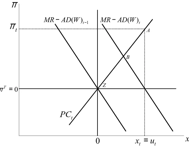
1. The first drawback is that from a teaching point of view the economy is not on theM R–AD W curve in periodtwhen the shock occurs (contrary to the way it is set out in Walsh). The reason is as follows: assume the economy was in equilibrium in periodt− . Then the central bank will not change the interest rate, r, in period t, since the central bank believes that nothing has changed to disturb the equilibrium. TheMR–AD W equation should really be written asxt −αβπCBt ut, since the monetary policy component of the
equation is equal to the level of output corresponding to the in ation rate the central bank believes it is imposing, namely hereπCB
t πT , so that the
xwhich the central bank believes it is producing isxCB
t . Hence output
will increase by exactlyut, so thatxt xCBt ut ut. In ation in periodt,
πt, is now determined by the intersection of the vertical linext utand the
Phillips curve. In Fig. 2 this is shown as pointA. PointB, the intersection of theM R–AD W curve in periodtand the Phillips curve in periodtis never reached. Note that B could only be reached if the central bank could reset rt. But if the central bank could reset rt, it would now be able to work out
the value ofutso that instead of moving toB, it would adjustrS,tup to take
account ofutand hence go straight toZ, the equilibrium point.
2. The second problem is not an analytic one but a pedagogical one and relates to the forward-looking way in which central banks function. We see this as re ecting the quite long time lags in the transmission of monetary policy. This is difficult to capture in Walsh’s model since there are no lags: i j . In our model, which we set out in the next sub-section, the rational central bank is engaged in forecasting the future. How one teaches undergraduates depends a lot on levels and background, but we have found it motivating for them to put themselves in the position of a central bank working out the future impact of its current actions.
2.5
The C–S model (
i
, j
)
t t
x
=
u
t
PC
1
( )t
MR−AD W − MR−AD W( )t
0
T
π =
t
π
x
π
0
A
B
Z
equations are as follows:
xt −a rt− −rS,t (ISequation)
πt πt− αxt (P C equation)
xt −αβπt . (M R–ADequation)
The IR equation is derived from the MR–AD equation using the Phillips curve equation to substitute forπt and theISequation to substitute forxt :
πt αxt −
αβxt
πt −
α β
αβ xt
rt−rS,t
αβ
a α β πt. (IRequation)
We shall show that this model does not suffer the drawbacks of the R–T and Walsh models. Irrespective of the kind of shock, in ation at the constant in ation equilibrium is equal to target in ation.6 Moreover, aggregate demand and supply shocks affect output and in ation and cannot be immediately offset by the central bank. The C–S model incorporates central bank optimization, and enables students to see that when the periodt CB sets rtit is having to forecast how to achieve its
desired values ofxt andπt . In Svensson’s language it is settingrtin response
to current shocks to meet ‘forecast targets’. Moreover, as we shall see in Section 3, there is a simple diagrammatic apparatus that students can use to explore how a wide variety of shocks and structural characteristics of the economy affect central bank decision-making.
2.6
The Svensson–Ball model (
i
, j
)
The Svensson–Ball model is the most realistic one, since its lag structure corre-sponds most closely to the views of central banks. For example, the Bank of Eng-land reports:
The empirical evidence is that on average it takes up to about one year in this and other industrial economies for the response to a mon-etary policy change to have its peak effect on demand and production, and that it takes up to a further year for these activity changes to have their fullest impact on the in ation rate.7
6We show in Section 4 how in ation bias arises if the central bank’s output target is above the
equilibrium,y .
Adopting our simplified treatment of the loss function (Section 2.1), the IS, P C andM R–ADequations in the Svensson–Ball model are:
xt −a rt− −rS,t (ISequation)
πt πt− αxt− (P C equation)
xt −δαβπt . (M R–ADequation)
As we have seen, it is possible to derive an interest rate rule that expresses how the central bank should react to current data. However, none of the lag structures examined so far delivers an interest rate equation that takes the form of Taylor’s em-pirical rule in which the central bank sets the interest rate in response to deviations in both output and in ation from target. The lag structure in the Svensson–Ball model produces an interest rate in the Taylor rule form:
xt −δαβπt
−a rt−rS,t −δαβπt −δα βxt
−δαβπt−δα βxt aδα β rt−rS,t
rt−rS,t
δαβ
a δα β πt αxt . (IRequation)
Hence the interest rate responds to current shocks to both output and in ation. In Taylor’s empirical rule, the weights on bothxtandπtare equal to 0.5: that will be
the case here ifδ α β a .
In spite of the advantage of greater realism, introducing the second lag (j ) to the C–S structure makes the diagrammatic analysis significantly harder because the Phillips curve has to be forecast a further period ahead. This does not pro-vide corresponding gains for students in terms of the basic insights of central bank behaviour.8
3
The C–S 3-equation model
In this section, we set out the C–S model to show how it can be taught to undergrad-uates. We present the model in a format useful for teaching, i.e. with the periods numbered zero and one and we work with output,y, rather than directly in terms of the output gap,x. The key lags in the system that the central bank must take into ac-count are shown in Fig. 3. In theIScurve, the choice of interest rate in period zero will only affect output next period (i ) as it takes time for interest rate changes to feed through to expenditure decisions. In the Phillips curve, this period’s in ation
y0
y1
r0
Phillips curve with inflation persistence
Lag from monetary policy to aggregate demand:
IS equation (i=1)
0
π
1
π
Policy instrument Contemporaneous
output in the Phillips curve (j=0)
Figure 3: The lag structure in the C–S 3-equation model
is affected by the current output gap (j ) and by last period’s in ation. The latter assumption of in ation persistence can be justified in terms of lags in wage- and or price-setting or by reference to backward-looking expectations: this assumption is common to all the models considered. The lag structure of the model explains why it is π andy that feature in the central bank’s loss function: by choosingr , the central bank determinesy , andy in turn determinesπ . This is illustrated in Fig. 3.
3.1
Equations
The three equations of the 3-equation model, the IS equation (#1), the Phillips curve equation (#2) and the MR–AD equation (#3), are set out in this section before being shown in a diagram. The central bank’s problem-solving can be dis-cussed intuitively and then depending on the audience, illustrated first either using the diagram or the algebra. The algebra is useful for pinning down exactly how the problem is set up and solved whereas the diagrammatic approach is well-suited to discussing different shocks and the path of adjustment to the new equilibrium.
requir-ing it to avoid large output uctuations:
L y −ye β π −πT . (Central Bank loss function)
The critical parameter isβ: β > will characterize a central bank that places less weight on output uctuations than on deviations in in ation, and vice versa. A more in ation-averse central bank is characterized by a higherβ.
The central bank optimizes by minimizing its loss function subject to the Phillips curve (j ):
π π α y −ye . (Inertial Phillips curve:P C equation, #2)
By substituting the Phillips curve equation into the loss function and differentiating with respect toy (which, as we have seen in Fig. 3, the central bank can choose by settingr ), we have:
∂L
∂y y −ye αβ π α y −ye −π
T
.
Substituting the Phillips curve back into this equation gives:
y −ye −αβ π −πT . (Monetary rule:M R–ADequation, #3)
This equation is the equilibrium relationship between the in ation rate chosen in-directly and the level of output chosen in-directly by the central bank to maximize its utility given its preferences and the constraints it faces.
To find out the interest rate that the central bank should set in the current period, we need to introduce theISequation. The central bank can set the nominal short-term interest rate directly, and since implicitly at least the expected rate of in ation is given in the short run, the central bank is assumed to be able to control the real interest rate indirectly. TheISequation incorporates the lagged effect of the interest rate on output (i ):
y A−ar (ISequation, #1)
and in output gap form is:
y −ye −a r −rS . (IS equation, output gap form)
If we substitute forπ using the Phillips curve in theM R–ADequation, we get
π α y −ye −πT −
αβ y −ye
π −πT − α
and if we now substitute for y −ye using theIS equation, we get
This tells the central bank how to adjust the interest rate (relative to the stabilizing interest rate) in response to a deviation of in ation from its target.
By setting out the central bank’s problem in this way, we have identified the key role of forecasting: the central bank must forecast the Phillips curve and the IS curve it will face next period. Although the central bank observes the shock in period zero and calculates its impact on current output and next period’s in ation, it cannot offset the shock in the current period because of the lagged effect of the interest rate on aggregate demand and output. This overcomes one of main draw-backs of the optimizing version of the R–T model. We therefore have a 3-equation model with an optimizing central bank in whichISshocks affect output.
3.2
Diagrams: the example of an
IS
shock
We shall now explain how the 3-equation model can be set out in a diagram. A graphical approach is useful because it allows students to work through the fore-casting exercise of the central bank and to follow the adjustment process as the optimal monetary policy is implemented and the economy moves to the new equi-librium.
The first step is to present two of the equations of the 3-equation model. In the lower part of the diagram, which we call the Phillips diagram, the vertical long-run Phillips curve at the equilibrium output level,ye, is shown. We think of labour
and product markets as being imperfectly competitive so that the equilibrium output level is where both wage- and price-setters make no attempt to change the prevailing real wage or relative prices. Each Phillips curve is indexed by the pre-existing or inertial rate of in ation,πI π
− .
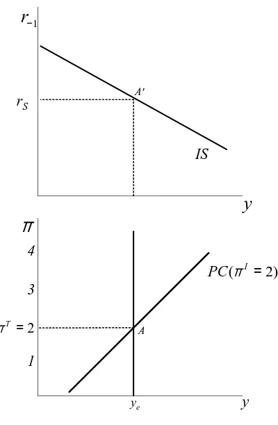
As shown in Fig. 4, the economy is in a constant in ation equilibrium at the output level of ye in ation is constant at the target rate ofπT and the real
interest rate required to ensure that aggregate demand is consistent with this level of output is the stabilizing rate,rS. Fig. 4 shows theIS equation in the upper panel:
the stabilizing interest rate will produce a level of aggregate demand equal to equi-librium output,ye. The interest rate axis in theISdiagram is labelledr− to capture
rS
IS
A A'
ye
4
3
1
π
2
T
π =
( I 2)
PC π =
1
r
−y
y
Figure 4: IS andP C curves
theIS curve, the Phillips curve and the central bank’s forecasting exercise to show how it formulates monetary policy.
In Fig. 5, we assume that as a consequence of an IS shock that shifts the IS curve toIS′, the economy is at point Ain the Phillips diagram with output above
equilibrium (aty ) and in ation ofπ above the target. The central bank’s job is to set the interest rate,r , in response to this new information about economic conditions. In order to do this, it must first make a forecast of the Phillips curve next period, since this shows the menu of output-in ation pairs that it can choose from by setting the interest rate now: remember that changing the interest rate now only affects output next period. Given that in ation is inertial, the central bank’s forecast of the Phillips curve in period one will beP C πI as shown by the dashed line
costly in the sense that output must be pushed below equilibrium in order to achieve disin ation.
How does the central bank make its choice from the combinations of in ation and output along the forecast Phillips curve (P C πI )? Its choice will depend
on its preferences: the higher isβ the more averse it is to in ation and the more it will want to reduce in ation by choosing a larger negative output gap. We show in the appendix how the central bank’s loss function can be represented graphically by loss circles or ellipses and we refer to the relevant parts of these circles or ellipses as its indifference curves. In Fig. 5, the central bank will choose point B at the tangency between its indifference curve and the forecast Phillips curve: this implies that its desired output level in period one is y . This level of output is the central bank’s aggregate demand target for period as implied by the monetary rule. The M R–ADline joins pointB and the zero loss point atZ, where in ation is at target and output is at equilibrium. The graphical construction of the downward sloping M R–ADline follows naturally from the economic reasoning.
The fourth step is for the central bank to forecast theIS curve for period one. In the example in Fig. 5, the forecast IS curve is shown by the dashed line and labelledIS′. With this IS curve, if an interest rate ofr′ is set in period zero, the
level of output in period one will bey as desired. Of course other random shocks may disturb the economy in period 1 but since these are by definition unforecastable by the central bank, they do not enter its decision rule in period zero.
To complete the example, we trace through the adjustment process. Following the increase in the interest rate, output falls to y and in ation falls to π . The central bank forecasts the new Phillips curve, which goes through point C in the Phillips diagram (not shown) and it will follow the same steps to adjust the interest rate downwards so as to guide the economy along the IS′ curve from C′ to Z′.
Eventually, the objective of in ation atπT is achieved and the economy is at
equilibrium output, where it will remain until a new shock or policy change arises. TheM R–ADline shows the optimal in ation-output choices of the central bank, given the Phillips curve constraint that it faces.
An important pedagogical question is the name to give the monetary rule equa-tion when we show it in the Phillips diagram. What it tells the central bank att is the output level that it needs to achieve int if it is to minimize the loss func-tion, given the forecast Phillips curve. Since we are explaining the model from the central bank’s viewpoint at t , what we want to convey is that the downward-sloping line in the Phillips diagram shows the aggregate demand target at t implied by the monetary rule. We therefore use the labelM R–AD.9
A set the interest rate in period 0.
4th: IS curve for period 1 is
forecast in period 0.
2nd: Phillips curve for period
1 is forecast in period 0.
3rd:Central bank calculates its
target output for period 1.
(
I2)
PC
π
=
1st: Inflation and output
are observed in period 0.
TheM R–ADcurve is shown in the Phillips diagram rather than in theIS dia-gram because the essence of the monetary rule is to identify the central bank’s best policy response to any shock. Both the central bank’s preferences shown graph-ically by its indifference curves and the Phillips curve trade-off it faces between output and in ation appear in the Phillips diagram. Once the central bank has cal-culated its desired output response by using the forecast Phillips curve, it is straight-forward to go to theISdiagram and discover what interest rate must be set in order to achieve this level of aggregate demand and output.
3.3
Using the graphical model
We now look at a variety of shocks so as to illustrate the role the following six elements play in their transmission and hence in the deliberations of policy-makers in the central bank:
1. the in ation target,πT
2. the central bank’s preferences,β
3. the slope of the Phillips curve,α
4. the interest sensitivity of aggregate demand,a
5. the equilibrium level of output,ye
6. the stabilizing interest rate,rS.
A temporary aggregate demand shock is a one-period shift in the IS curve, whereas a permanent aggregate demand shock shifts the IS curve and hence rS,
the stabilizing interest rate, permanently. An in ation shock is a temporary (one-period) shift in the short-run Phillips curve. This is sometimes referred to as a temporary aggregate supply shock. An aggregate supply shock refers to a perma-nent shift in the equilibrium level of output, ye. This shifts the long-run vertical
Phillips curve.
If aggregate demand shocks int are included, the curve ceases to be the curve on which the central bank bases its monetary policy int . On the other hand if an aggregate demand shock int is excluded — so that the central bank can base monetary policy on the curve — then it is misleading to call it theADschedule students would not unreasonably be surprised if anAD
3.3.1 ISshock: temporary or permanent?
In Section 3.2 and Fig. 5 we analyzed anIS shock — but was it a temporary or a permanent one? In order for the central bank to make its forecast of theIScurve, it has to decide whether the shock that initially caused output to rise toy is temporary or permanent. In our example, the central bank took the view that the shock would persist for another period, so it was necessary to raise the interest rate to r′ above
the new stabilizing interest rate,r′
S. Had the central bank forecast that theIScurve
would revert to the pre-shock IS curve, then it would have raised the interest rate by less since the stabilizing interest rate would have remained unchanged at rS.
The chosen interest rate would have been on theIScurve labelled pre-shock at the output level ofy (see Fig. 5).
3.3.2 Supply shock
One of the key tasks of a basic macroeconomic model is to help illuminate how the main variables are correlated following different kinds of shocks. We can appraise the usefulness of the IS-PC-MR model in this respect by looking at a positive ag-gregate supply shock and comparing the optimal response of the central bank and hence the output and in ation correlations with those associated with an aggre-gate demand shock. A supply shock results in a change in equilibrium output and therefore a shift in the long-run Phillips curve. It can arise from changes that af-fect wage- or price-setting behaviour such as a structural change in wage-setting arrangements, a change in taxation or in unemployment benefits or in the strength of product market competition, which alters the mark-up.
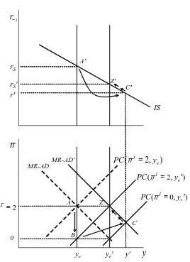
Fig. 6 shows the analysis of a positive supply-side shock, which raises equilib-rium output fromyetoye′. Before analyzing the impact of the shock and the
adjust-ment process as the central bank works out and impleadjust-ments its optimal response, it is useful to identify the characteristics of the new constant-in ation equilibrium. In the new equilibrium, equilibrium output will be at the new higher level,y′
e, and
in ation will be at its target of . The long-run Phillips curve will be aty′
e. There
will a newMR–ADcurve,M R–AD′, since it must go through the in ation target
and the new equilibrium output level, y′
e: the zero loss point for the central bank
following this shock is at point Z. Note also that as a consequence of the supply shock, the stabilizing interest rate has fallen tor′
S.
We now examine the initial effect of the shock. Since the long-run Phillips curve shifts to the right so too does the short-run Phillips curve corresponding to in ation equal to the target (shown by the P C πI , y′
e ). The first consequence of the
in period zero. To decide how monetary policy should be adjusted to respond to this, we follow the same steps taken in Section 3.2. The central bank forecasts the Phillips curve constraint (P C πI , y′
e ) for period one and chooses its optimal
level of output as shown by pointC. Next the central bank must forecast the IS curve: since there is no information to suggest any shift in theIS curve, it is as-sumed fixed. To raise output to the level desired, the central bank must therefore cut the interest rate in period zero tor′ as shown in theISdiagram. Note that since
the stabilizing interest rate has fallen tor′
S, the central bank reduces the interest rate
below this in order to achieve its desired output level ofy′. The economy is then
guided along theM R–AD′curve to the new equilibrium atZ.
The positive supply shock is associated initially with a fall in in ation, in con-trast to the initial rise in both output and in ation in response to the positive ag-gregate demand shock. In the agag-gregate demand case, the central bank has to push output below equilibrium during the adjustment process in order to squeeze the higher in ation caused by the demand shock out of the economy. Conversely in the aggregate supply shock case, a period of output above equilibrium is needed in order to bring in ation back up to the target from below. In the new equilibrium, output is higher than its initial level in the supply shock case whereas it returns to its initial level in the case of the aggregate demand shock. In the new equilibrium, in ation is at target in both cases. However, whereas the real interest rate is higher than its initial level in the new equilibrium following a permanent positive aggregate demand shock, it is lower following a positive aggregate supply shock.
3.3.3 ISshock: the role of the interest-sensitivity of aggregate demand
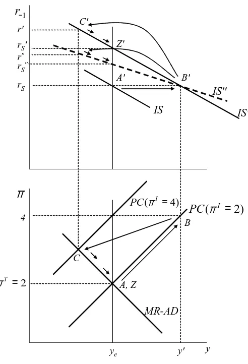
In the next experiment (Fig. 7), we keep the supply side of the economy and the central bank’s preferences fixed and examine how the central bank’s response to a permanent aggregate demand shock is affected by the sensitivity of aggregate demand to the interest rate. It is assumed that the economy starts off with output at equilibrium and in ation at the target rate of 2%. The economy is atA′ in theIS
diagram and atAin the Phillips diagram. The equilibrium is disturbed by a positive aggregate demand shock such as improved buoyancy of consumer expectations, which is assumed by the central bank to be permanent. Two post-shockIScurves are shown in the upper panel of Fig. 7: the more interest sensitive one is the atter one labelledIS′′. To prevent the diagram from getting too cluttered, only the steeper
of the two pre-shockIS curves is shown.
The step-by-step analysis of the impact of the shock is the same as in Section 3.2. The consequence of output aty′ above y
e is that in ation rises above target
ye'
rS
r'
MR-AD
IS
A
B
Z
C A'
C' Z'
y' ye
MR-AD'
0
rS'
π
1
r−
y
2 T
π =
( I 2, e)
PC π = y
( I 2, e )
PC π = y′
( I 0, )
e PCπ = y ′
rS r''
MR-AD
A, Z
B
C
A' C'
Z'
y' ye
4 rS'
B'
IS' IS''
rS''
r'
( I 4)
PC π =
( I 2)
PC π =
2 T
π =
π
y
1
r−
IS
its preferred point for the next period: pointC. Since the supply side and the cen-tral bank’s preferences are assumed to be identical for each economy, the Phillips diagram and hence theP C and MR–AD curves are common to both. However, in the next step, the structural difference between the two economies is relevant. By going vertically up to the IS diagram, we can see that the central bank must raise the interest rate by less in response to the shock (i.e. tor′′rather than tor′) if
aggregate demand is more responsive to a change in the interest rate (as illustrated by the atterIS curve,IS′′).
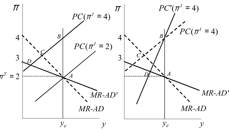
3.3.4 How central bank in ation aversion and the slope of the Phillips curve
affect interest rate decisions
To investigate how structural features of the economy such as the degree of in a-tion aversion of the central bank and the responsiveness of in aa-tion to the output gap impinge on the central bank’s interest rate decision, we look at the central bank’s response to an in ation shock. A one-period shift in the Phillips curve could occur as a result, for example, of an agricultural disease outbreak that temporarily inter-rupts supply and pushes in ation above the target level. We assume the economy is initially in equilibrium with output ofyeand in ation at the central bank’s target
rate of . This is shown by pointAin each panel of Fig. 8. To prevent cluttering the diagrams, the initial short-run Phillips curve is only shown in Fig. 8(a). The economy experiences a sudden rise in in ation to . The short-run Phillips curve shifts toP C πI and the economy moves to pointB in Fig. 8.
In our first example in Fig. 8(a), we focus attention on the consequences for monetary policy of different degrees of in ation aversion on the part of the central bank (β): the other five structural characteristics listed at the beginning of Section 3.3 are held constant. From theM R–ADequation (i.e. y −ye −αβ. π −πT )
and from the geometry in Fig. 11 in the appendix, it is clear that if the indifference curves are circles (i.e. β ) and if the Phillips curve has a gradient of one (i.e. α ), the M R–AD line is downward sloping with a gradient of minus one. It follows that theM R–ADline will be atter than this if the weight on in ation in the central bank’s loss function is greater than one (β > ). The more in ation-averse central bank is represented by the solidM R–AD′ line in Fig. 8(a). In response to
the in ation shock, the more in ation-averse central bank wishes to reduce in ation by more and will therefore choose a larger output reduction: pointDas compared with pointCfor the less in ation-averse central bank.
the steeper Phillips curve (α > ) shown by the solid line has the atter MR–AD curve: this is the solid one labelledM R–AD′. As in Fig. 8(a), the in ation shock
shifts the short run Phillips curve upwards and takes the economy from pointAto pointB on the long-run Phillips curve. Whenα (i.e. with the dashed Phillips curve andM R–ADcurve), the central bank’s optimal point isC, whereas we can see that if the Phillips curve is steeper, the central bank cuts aggregate demand by less (pointD). The intuition behind this result is that a steeper Phillips curve means that, holding central bank preferences constant, it has to ‘do less’ in response to a given in ation shock since in ation will respond sharply to the fall in output asso-ciated with tighter monetary policy.
Using the diagram underlines the fact that although theMR–ADcurve is atter in both of our experiments, i.e. with a more in ation-averse central bank or with greater sensitivity of in ation to output, the central bank’s reaction to a given in a-tion shock is different. In the left hand panel, the atterMR–AD curve is due to greater in ation-aversion on the part of the central bank. Such a central bank will always wish to cut output by more in response to a given in ation shock (choosing pointD) as compared with the neutral case of β (where pointC will be cho-sen). By contrast in the right hand panel, a central bank facing a more responsive supply-side (as re ected in steeper Phillips curves) will normally choose to do less in response to an in ation shock (choosing pointD) than would a central bank with the same preferences facing a less responsive supply-side (pointC).
The examples in Fig. 8(b) and Fig. 7 highlight that if we hold the central bank’s preferences constant, common shocks will require different optimal responses from the central bank if the parametersα(re ected in the slope of the short run Phillips curve) ora(re ected in the slope of theIScurve) differ. This is relevant to the com-parison of interest rate rules across countries and to the analysis of monetary policy in a common currency area. For example in a monetary union, unless the aggregate supply and demand characteristics that determine the slope of the Phillips curve and the IS curve in each of the member countries are the same, the currency union’s interest rate response to a common shock will not be optimal for all members.
3.4
Lags and the Taylor rule
3
4
y
eB
MR-AD'
MR-AD
π
C D
a. Greater inflation-aversion
y
(
I4)
PC
π
=
3
4
y
eB
MR-AD'
MR-AD
π
2
T
π
=
C
D
b. Steeper Phillips curve
y
(
I4)
PC
′
π
=
(
I4)
PC
π
=
(
I2)
PC
π
=
A A
coefficients . and . :
r −rS . π −πT . y −ye . (Taylor rule)
We derived the Taylor-type rule for the 3-equation C–S model:
r −rS
immediately apparent: first, only the in ation and not the output deviation is present in the rule although the central bank cares about both in ation and output deviations as shown by its loss function. Second, as we have seen in the earlier examples, all the parameters of the three equation model matter for the central bank’s optimal response to a rise in in ation. If each parameter is equal to one, the weight on the in ation deviation is one half. For a given deviation of in ation from target, and in each case, comparing the situation with that in whicha α β , we have
• a more in ation averse central bank (β > ) will raise the interest rate by more
• when theIS is atter (a > ), the central bank will raise the interest rate by less
• when the Phillips curve is steeper (α > ), the central bank will raise the interest rate by less.10
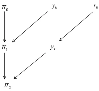
As shown in the discussion of the Svensson–Ball model in Section 2, in order to derive a Taylor rule in which both in ation and output deviations are present, it is necessary to modify the lag structure of the three equation C–S model. Specifically, it is necessary to introduce an additional lag (j ), i.e. the output levely affects in ation a period later,π . This means that it isy and noty that is in the Phillips curve forπ .
The double lag structure is shown in Fig. 9 and highlights the fact that a decision taken today by the central bank to react to a shock will only affect the in ation rate two periods later, i.e. π . When the economy is disturbed in the current period (period zero), the central bank looks ahead to the implications for in ation and sets the interest rater so as to determiney , which in turn determines the desired value of π . As the diagram illustrates, action by the central bank in the current period has no effect on output or in ation in the current period or on in ation in a year’s time.
y0
y1
r0
2
π
0
π
1
π
Figure 9: Double lag structure in the 3-equation model (i j )
Given the double lag (i j ), the central bank’s loss function containsy and π since it is these two variables it can choose through its interest rate deci-sion:11
L y −ye β π −πT
and the three equations are:
π π α y −ye (Phillips curve)
y −ye −a r −rS (IS )
π −πT −
αβ y −ye . (M R–AD)
By repeating the same steps as we used in Section 2.1, we derive the interest rate rule:
r −rS
αβ
a α β π −π
T α y −y e .
(Interest rate (Taylor) rule in 3-equation (double lag) model)
11For clarity when teaching, it is probably sensible to ignore the discount factor, i.e. we assume
We note that Taylor’s empirical formulation emerges ifa α β , i.e.
r −rS . π −πT . y −ye .
Implicitly the interest rate rule incorporates changes in the interest rate that are required as a result of a change in the stabilizing interest rate (in the case of a permanent shift in the IS or of a supply-side shift): rS in the rule should be
interpreted as the post-shock stabilizing interest rate.
It is often said that the relative weights on output and in ation in a Taylor rule re ect the central bank’s preferences for reducing in ation as compared to output deviations. However, we have already seen in the single lag version of the model that although the central bank cares about both in ation and output deviations, only the in ation deviation appears in the interest rate rule. Although both the output and in ation deviations are present in the IR equation for the double lag model, the relative weights on in ation and output depend only on α, the slope of the Phillips curve. The relative weights are used only to forecast next period’s in ation. The central bank’s preferences determine the interest rate response to next period’s in ation (as embodied in the slope of theM Rcurve). Another way to express this result is to say that the output term only appears in theIRequation because of the lag from a change in output to a change in in ation, i.e. becausej .
4
In ation bias and time inconsistency
4.1
Introducing in ation bias
In the 3-equation models analyzed to this point (with the exception of the R–T model without an optimizing central bank), medium-run equilibrium is character-ized by in ation equal to the central bank’s in ation target and by output at equilib-rium. However, since imperfect competition in product and labour markets implies thatyeis less than the competitive full-employment level of output, the government
may have a higher target output level. We assume that the government can impose this target on the central bank. How do things change if the central bank’s target is full-employment output, or more generally a level of output aboveye? For clarity,
we use the C–S model (i , j ).
A starting point is to look at the central bank’s new objective function. It now wants to minimize
L y −yT β π −πT , (1)
whereyT > y
e. This is subject as before to the Phillips curve,
y
the supply side of the economy, the Phillips curves remain unchanged. To work out the central bank’s monetary rule, consider the level of output it chooses ifπI .
Fig. 10 shows the Phillips curve corresponding to πI . The tangency of
P C πI with the central bank’s indifference curve shows where the central
bank’s loss is minimized (point D). Since the central bank’s monetary rule must also pass throughA, it is the downward sloping lineMR–ADin Fig. 10.
We can see immediately that the government’s target, pointA, does not lie on the Phillips curve for inertial in ation equal to the target rate of πT : the
economy will only be in equilibrium with constant in ation at point B. This is where the monetary rule (M R–AD) intersects the vertical Phillips curve aty ye.
At point B, in ation is above the target and the gap between the target rate of in ation and in ation in the equilibrium is the in ation bias.
We shall now pin down the source of in ation bias and the determinants of its size. We begin by showing why the equilibrium is at point B. If the economy is initially at pointC with output at equilibrium and in ation at its target rate of , the central bank chooses its preferred point on the P C πI and the economy
up to and the Phillips curve for the following period shifts up (see the dashed Phillips curve in Fig. 10). The process of adjustment continues until point B is reached: output is at the equilibrium and in ation does not change so the Phillips curve remains fixed. Neither the central bank nor price- or wage-setters have any incentive to change their behaviour. The economy is in equilibrium. But neither in ation nor output are at the central bank’s target levels (see Fig. 10). In ation bias arises because target output is aboveye: in equilibrium, the economy must be
at the output level ye and on theM R–ADcurve. It is evident from the geometry
that a steeperMR-ADline will produce a larger in ation bias.
We can derive the same result using the equations. Minimising the central bank’s loss function (equation (1)) subject to the Phillips curve (equation (2)) im-plies
y −yT αβ π α y −ye −πT y −yT αβ π −πT
.
So the new monetary rule is:
y −yT −αβ π −πT . (M R–ADequation)
This equation indeed goes through (πT, yT . Since from the Phillips curve, we have
π π wheny ye, it follows that
ye yT −αβ π −πT
⇒ π πT yT −ye
αβ in ation bias
. (In ation bias)
In equilibrium, in ation will exceed the target by yαβ−y , the in ation bias.12 The significance of this result is thatπ > πT wheneveryT > y
e. In other words, it is
the fact that the central bank’s output target is higher than equilibrium output that is at the root of the in ation bias problem. In ation bias will be greater, the less in ation-averse it is i.e. the lower is β. A lower α also raises in ation bias. A lower α implies that in ation is less responsive to changes in output. Therefore, any given reduction in in ation is more expensive in lost output so in cost-benefit terms for the central bank, it pays to allow a little more in ation and a little less output loss.
12For an early model of in ation bias with backward-looking in ation expectations, see Phelps
4.2
Time inconsistency and in ation bias
The problem of in ation bias is usually discussed in conjunction with the problem of time inconsistency in which the central bank or the government announces one policy but has an incentive to do otherwise. For this kind of behaviour to arise, it is necessary to introduce forward-looking in ation expectations. The simplest as-sumption to make is that in ation expectations are formed rationally and that there is no in ation inertia: i.e. πE E π, soπ πE ε
t, whereεt is uncorrelated
withπE. We continue to assume that the central bank choosesy(and henceπ) after
private sector agents have chosenπE. This defines the central bank as acting with
discretion. Now, in order for firms and workers to have correct in ation expecta-tions, they must chooseπE such that it pays the central bank to choosey y
e. That
must be where the central bank’s monetary rule cuts they yevertical line, i.e. at
pointBin Fig. 10. Note that the positively sloped lines are now interpreted as Lu-cas supply equations rather than as short-run Phillips curves.13 This is the so-called Lucas surprise supply equation:
For an expectations equilibrium, in ation must be sufficiently high to remove the temptation of the central bank to raise output toward its target. With π
andy ye, the temptation has been removed because any increase in output from
B would put the central bank on a loss circle more distant from its bliss pointA: firms and workers therefore rationally expect an in ation surprise of over and above the target in ation rate of (compare point B, which is an expectations equilibrium for the private sector and the central bank, with pointC, which is not an equilibrium for the central bank).
In ation bias presents a problem. As is clear from Fig. 10, the loss to the central bank atBis greater than its loss atC, since output is the same but in ation is higher atB. So the central bank would clearly be better off atC. Moreover, firms and workers would be just as happy at C as at B, since output, employment and the real wage are the same in each case. What is to stop the central bank being at C? When private sector agents are forward-looking, the problem is called that of time inconsistency. Although the central bank claims to have an in ation target of
13The usual interpretation of the former is that an in ation surprise leads output to deviate from
πT, if firms and workers act on the basis of this target ( ), when it comes to set
the interest rate, the central bank does not choose the output level consistent with its target. In short, at point B there is no incentive for the central bank to cheat whereas at pointC, there is an incentive.
5
Conclusions
In Section 2 we showed how different versions of a simplified 3-equation New Key-nesian model were generated by the absence or presence of two critical time-lags — from the interest rate to output (i or ) and from output to in ation (j or ). Thus the simple Romer–Taylor model hasi andj Walsh has i j and Svensson–Ball has i j . Our preferred model for teaching purposes (C–S) hasi andj . The paper develops this model graphically as a replac-ment for the standard IS-LM-AS model. It provides undergraduate students and non-specialists with the tools for analyzing a wide range of macroeconomic distur-bances and with access to contemporary debates in the more specialized monetary macroeconomics literature. It has a number of features that distinguish it from other models that replace the LM equation with a monetary policy rule. First, it conforms with the view that monetary policy is conducted by optimizing forward-looking central banks. Second, since aggregate demand responds to interest rate changes with a lag, aggregate demand and aggregate supply shocks cannot be fully offset even by a forward-looking central bank. Third, in response to a shock, the central bank guides the economy back to equilibrium with target in ation.
The graphical approach helps illuminate the role played by structural character-istics of the aggregate supply and demand sides of the economy and by the central bank’s preferences in determining the optimal interest rate response to shocks. It is straightforward to demonstrate the determinants of the size of the in ation bias using this model and the origin of the time inconsistency problem.
y
ye ye y ye y
(a) Balanced: ß =1 (b) Inflation-averse: ß >1
(c) Unemployment-averse: ß <1
π
π
π
T
π πT πT
Figure 11: Central bank loss function: varying the degree of in ation aversion
6
Appendix
The central bank’s loss function: graphical representation
The geometry of the central bank’s loss function can be shown in the Phillips diagram. The loss function withi , j , i.e.
L y −ye β π −πT ,
is simple to draw. Withβ , each indifference curve is a circle with (ye, πT) at its
centre (see Fig. 11(a)). The loss declines as the circle gets smaller. Whenπ πT
andy ye, the circle shrinks to a single point (called the ‘bliss point’) and the loss
is zero. Withβ , the central bank is indifferent between in ation above (or below)πT and output below (or above)y
e. They are on the same loss circle.
Only whenβ , do we have indifference circles. Ifβ > , the central bank is indifferent between (say) in ation above (or below)πT and output above (or
below)ye.This makes the indifference curves ellipsoid as in Fig. 11(b). A central
off a given fall in in ation for a smaller fall in output than in the other two cases. Such a central bank is sometimes referred to as unemployment-averse.
7
References
Allsopp, Christopher and David Vines (2000). ‘The Assessment: Macroeco-nomic Policy’. Oxford Review of EcoMacroeco-nomic Policy 16(4): 1-32.
Ball, Lawrence (1999). ‘Efficient Rules for Monetary Policy’. International Finance 2(1): 63-83.
Bank of England (1999). ‘The Transmission of Monetary Policy’.
http://www.bankofengland.co.uk/publications/other/monetary/montrans.pdf. Carlin, Wendy and David Soskice (2006). Macroeconomics: Imperfections, Institutions, and Policies. Oxford: Oxford University Press.
Clarida, Richard, Jordi Gali and Mark Gertler (1999). ‘The Science of Monetary Policy: A New Keynesian Perspective’. Journal of Economic Literature 37(4): 1661-1707.
Goodfriend, Marvin and Robert King (1997). ‘The New Neoclassical Synthesis and the Role of Monetary Policy’. NBER Macroeconomics Annual 12: 231-283.
Gürkaynak, Refet, Andrew Levin and Eric Swanson (2005). ‘Does In ation Targeting Anchor Long-Run In ation Expectations? Evidence from Long-Term Bond Yields in the US, UK and Sweden’. Unpublished Manuscript, Federal Re-serve Bank of San Francisco.
Phelps E. S. (1967). ‘Phillips Curves, Expectations of In ation and Optimal Unemployment over Time’. Economica New Series 34/135: 254-281.
Romer, David (2000). ‘Keynesian Macroeconomics without the LM Curve’. Journal of Economic Perspectives 14(2): 149-169.
Svensson, Lars E.O. (1997). ‘In ation Forecast Targeting: Implementing and Monitoring In ation Targets’. European Economic Review 41(6): 1111-1146.
Taylor, John B. (1993). ‘Discretion Versus Policy Rules in Practice’. Carnegie-Rochester Conference Series on Public Policy 39(1): 195-214.
Taylor, John B. (2000). ‘Teaching Modern Macroeconomics at the Principles Level’. American Economic Review Papers and Proceedings 90(2), 90-94.
Walsh, Carl E. (2002). ‘Teaching In ation Targeting: An Analysis for Interme-diate Macro’. Journal of Economic Education 33(4): 333-347.