Optimal Power Flow Enhancement Considering
Contingency with Allocate FACTS
Rakhmad Syafutra Lubis1,*, Sasongko Pramono Hadi2, Tumiran2
1PhD Student in Electrical Engineering and Information Technology, Gadjah Mada University, Yogyakarta, 55281, Indonesia 2Electrical Engineering and Information Technology, Gadjah Mada University, Yogyakarta, 55281, Indonesia
Abstract This paper presents techniques for OPF-based electricity market enhancement with considering contingencies,
allocating the Flexible AC Transmission System (FACTS) and estimating the system-wide available transfer capability (SATC) computations. The voltage stability constraints optimal power flow (VSC-OPF) problem formulation installs with the FACTS and includes the loading parameter in order to ensure enhancement a proper stability margin for the market solution. The first technique is an iterative approach and computes the SATC value based on the 𝑁𝑁 −1 contingency criterion for an initial optimal operating condition, to then solve an OPF problem for the worst contingency case; this process is repeated until the changes in the SATC values are below a minimum threshold. The second technique solves a reduced number of OPF associated with contingency cases according to a ranking based on the power transfer sensitivity analysis. Both techniques are tested on the IEEE 14-bus test system considering locational marginal prices (LMP) and nodal congestion prices (NCP) and then compared with results obtained by means of the VSC-OPF considering 𝑁𝑁 −1contingency criteria technique without installing the FACTS. A good system response for the allocated the FACTS devices which indicates that the devices given a powerful response for the VSC-OPF method, the two method, with presenting the security method and the transaction method result in improved transactions, higher security margins and lower prices.
Keywords Electricity markets, Optimal power flow,
N−1 contingency criterion, FACTS, Available transfer capability1. Introduction
In competitive market structures, such as centralized markets, standard auction markets, and spot-pricing or hybrid markets, the several studies have been published regarding the definition of a complete market model able to account for both economic and security aspects. Furthermore, the inclusion of the “correct” stability constraints and the determination of fair security prices have been properly addressed with so far so good. However, the inclusion of the FACTS devices for improving the techniques has not been addressed.
Reliability of the FACTS devices for enhancement the VSC-OPF performance included N-1 contingency criteria is focus of discussion in this paper. The hybrid markets and the two methods for the contingencies and stability constraints through the use of the VSC-OPF have been presented[1]. The OPF problem has been solved using an interior point method (IPM) that has proven to be robust and reliable for realistic size networks[2]. A proper representation of voltage stability constraints and maximum loading conditions, which may be associated with limit-induced bifurcations or
* Corresponding author:
[email protected] (Rakhmad Syafutra Lubis) Published online at http://journal.sapub.org/ijee
Copyright © 2013 Scientific & Academic Publishing. All Rights Reserved
saddle-node bifurcations, is used to represent the stability constraints in the OPF problem[3]. This technique has been applied to solve diverse OPF market problems as demonstrated in[1, 4].
Some studies for contingency planning and voltage security preventive control have been presented in[5], and the OPF computations with inclusion of voltage stability constraints and contingencies without installing the FACTS [1, 6] have also been discussed. However, the accounting of system contingencies in the VSC-OPF market problem with installing the FACTS has not arranged in the technical publication.
This paper uses the technique to account for system security through the use of voltage-stability-based constraints and the estimation of the system congestion through the value of the SATC as proposed in[1, 7] to OPF enhancement. In this case, voltage and power transfer limits are not computed off-line, which is the current common strategy, but are properly represented in on-line market computations by means of the inclusion of a loading parameter in the system stability constraints.
methodology to ensure transient stability that relies on an OPF model with inclusion of transient stability constraints (TSC) in the OPF that based on the using of the concept of single machine equivalent (SIME) method and ensure transient stability of the system against major disturbances, e.g., faults and/or line outages[9]. Furthermore the incorporating the N-1 security criterion in order to reduce the size of the resulting OPF problem, a prior contingency filtering is used for reducing the size of the small-signal stability constrained OPF (SSSC-OPF) problem, where only incorporate contingencies that threaten system stability[10].
In this paper, the basic technique initially proposed in[11] and expanded in[1] with include contingencies, such that an accurate evaluation of the SATC can be obtainedis further developed to include the FACTS devices, such that an enhancement the technique in[1] can be obtained.
The paper is organized as follows. Section 2 presents the mathematical model of the FACTS devices. Section 3 presents the basic concepts on which the methodologies are based that cited by means in[1] and advanced by applying the FACTS devices; the definitions of local marginal prices and nodal congestion prices and of SATC are also discussed by means of the literature in[1]. Furthermore in Section 3 discusses two techniques to account for contingencies in the OPF problem, with particular emphasis on their application to OPF-based electricity market models and then advances to allocate the FACTS devices. The applications of the proposed techniques are demonstrated in Section 4for the IEEE 14-Bus test system assuming elastic demand bidding; for the test systems, results are compared with respect to solutions obtained with the standard OPF-based market technique without the FACTS and with the VSC-OPF based market technique included N-1 contingency criteria without the FACTS devices respectively. Finally, Section 5resumes the conclusions as the main contributions of this paper as well as describes possible future research directions.
2. Mathematical Model of the FACTS
Devices
Power Injection Model of the FACTS: The power-injected model is a good model for FACTS devices because it will handle them well in load flow computation problem. Since, this method will not destroy the existing impedance matrix Z; it would be easy while implementing in load flow programs. In fact, the injected power model is convenient and enough for power system with FACTS devices. The Mathematical models of the FACTS devices are developed mainly to perform the steady-state research. The SVC and TCSC are modeled using the power injection method[12] and UPFC [13].
2.1. The FACTS Devices
In an interconnected power system network, power flows obey the Kirchhoff’s laws. The resistance of the transmission line is small compared to the reactance. Also the transverse
conductance is close to zero. The active power transmitted by a line between the buses 𝑖𝑖 and 𝑗𝑗 may be approximated by following relationships:
𝑃𝑃𝑖𝑖𝑗𝑗 =𝑉𝑉𝑋𝑋𝑖𝑖𝑉𝑉𝑖𝑖𝑗𝑗𝑗𝑗sin𝛿𝛿𝑖𝑖𝑗𝑗 (1) or ∆𝑃𝑃=∆𝑋𝑋
𝑋𝑋 ∙ 𝑃𝑃+ ∆𝑉𝑉
𝑉𝑉 ∙ 𝑃𝑃+ ∆𝜙𝜙
tan𝜙𝜙∙ 𝑃𝑃
where: 𝑉𝑉𝑖𝑖 and 𝑉𝑉𝑗𝑗 are voltages at buses i and j; 𝑋𝑋𝑖𝑖𝑗𝑗 : reactance of the line; 𝛿𝛿𝑖𝑖𝑗𝑗: angle between the 𝑉𝑉𝑖𝑖 and 𝑉𝑉𝑗𝑗. Under the normal operating condition for high voltage line the voltage 𝑉𝑉𝑖𝑖 and 𝑉𝑉𝑗𝑗 and 𝛿𝛿𝑖𝑖𝑗𝑗 is small. The active power flow coupled with 𝛿𝛿𝑖𝑖𝑗𝑗 and reactive power flow is linked with difference between the 𝑉𝑉𝑖𝑖 and 𝑉𝑉𝑗𝑗. The control of 𝑋𝑋𝑖𝑖𝑗𝑗 acts on both active and reactive power flows. The different types of FACTS devices have been choose and locate optimally in order to control the power flows in the power system network. The SVC can be used to control the reactive power. The reactance of the line can be changed by the TCSC. The TCPAR varies the phase angle between the two terminal voltages. The UPFC is most power full and versatile device, which control line reactance, terminal voltage, and the phase angle between the buses. In this paper, three different typical FACTS are selected: SVC, TCSC and UPFC.
2.2. Mathematical Model of the SVC
Power Injection Model of the SVC: SVC can control bus voltage and inject reactive power, modelled by power injection model as example is effective to hold the voltage fluctuation in starting and stopping action of generator.
In this model, a total reactance bSVC is assumed and the
following differential equation holds
𝑏𝑏̇𝑆𝑆𝑉𝑉𝑆𝑆 =�𝐾𝐾𝑟𝑟�𝑉𝑉𝑟𝑟𝑟𝑟𝑟𝑟 +𝑣𝑣𝑃𝑃𝑃𝑃𝑃𝑃− 𝑉𝑉� − 𝑏𝑏𝑆𝑆𝑉𝑉𝑆𝑆� 𝑇𝑇⁄ 𝑟𝑟 (2) The model is completed by the algebraic equation expressing the reactive power injected at the SVC node:
𝑄𝑄=𝑏𝑏𝑆𝑆𝑉𝑉𝑆𝑆𝑉𝑉2 (3) The regulator has an anti-windup limiter, thus the reactance bSVC is locked if one of its limits is reached and
the first derivative is set to zero.
2.3. Mathematical Model of the TCSC
Power Injection Model of the TCSC: The algebraic equations of the basic TCSC structure with current control are:
𝑃𝑃𝑖𝑖𝑗𝑗 =𝑉𝑉𝑖𝑖𝑉𝑉𝑗𝑗�𝑌𝑌𝑖𝑖𝑗𝑗 +𝐵𝐵�sin�𝜃𝜃𝑖𝑖− 𝜃𝜃𝑗𝑗�
𝑃𝑃𝑖𝑖𝑗𝑗 =−𝑃𝑃𝑗𝑗𝑖𝑖
𝑄𝑄𝑖𝑖𝑗𝑗 =𝑉𝑉𝑖𝑖2�𝑌𝑌
𝑖𝑖𝑗𝑗 +𝐵𝐵� − 𝑉𝑉𝑖𝑖𝑉𝑉𝑗𝑗�𝑌𝑌𝑖𝑖𝑗𝑗 +𝐵𝐵�cos�𝜃𝜃𝑖𝑖− 𝜃𝜃𝑗𝑗� 𝑄𝑄𝑗𝑗𝑖𝑖 =𝑉𝑉𝑗𝑗2�𝑌𝑌𝑖𝑖𝑗𝑗 +𝐵𝐵� − 𝑉𝑉𝑖𝑖𝑉𝑉𝑗𝑗�𝑌𝑌𝑖𝑖𝑗𝑗 +𝐵𝐵�cos�𝜃𝜃𝑖𝑖− 𝜃𝜃𝑗𝑗� (4)
where 𝑌𝑌𝑖𝑖𝑗𝑗 is the admittance of the line at which the TCSC is connected, and the indexes i and j stand for the sending and receiving bus indices, respectively.
The TCSC differential equations are as follows:
𝑥𝑥̇2=𝐾𝐾𝐼𝐼�𝑃𝑃𝑖𝑖𝑗𝑗 − 𝑃𝑃𝑟𝑟𝑟𝑟𝑟𝑟� (5) where: {𝑥𝑥𝑆𝑆0,𝛼𝛼0} =𝐾𝐾𝑃𝑃�𝑃𝑃𝑖𝑖𝑗𝑗− 𝑃𝑃𝑟𝑟𝑟𝑟𝑟𝑟�+𝑥𝑥2
The state variables 𝑥𝑥1= {𝑥𝑥𝑆𝑆0,𝛼𝛼0} depend on the TCSC model. The PI controller is enabled only for the constant power flow operation mode. The output signal is the series susceptance B of the TCSC, as:
𝐵𝐵(𝑥𝑥𝑆𝑆) =− 𝑥𝑥𝑆𝑆⁄𝑥𝑥𝑖𝑖𝑗𝑗 𝑥𝑥𝑖𝑖𝑗𝑗�𝐼𝐼 − 𝑥𝑥𝑆𝑆⁄ �𝑥𝑥𝑖𝑖𝑗𝑗
During the power flow analysis the TCSC is modeled as a constant capacitive reactance that modifies the line reactance
𝑥𝑥𝑖𝑖𝑗𝑗 as follows:
𝑥𝑥′𝑖𝑖𝑗𝑗 =�1− 𝑐𝑐𝑝𝑝�𝑥𝑥𝑖𝑖𝑗𝑗
where 𝑐𝑐𝑝𝑝 is the percentage of series compensation. The TCSC state variables are initialized after the power flow analysis as well as the reference power of the PI controller
𝑃𝑃𝑟𝑟𝑟𝑟𝑟𝑟. At this step, a check of 𝑥𝑥𝑐𝑐 and/or 𝛼𝛼 anti-windup limits is performed. In case of limit violation a warning message is displayed. Initialization a check for SVC limits is performed.
2.4. Mathematical Model of the UPFC
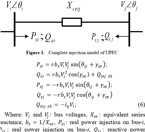
Power Injection Model of the UPFC: A series inserted voltage and phase angel of inserted voltage can model the effect of UPFC on network. The inserted voltage has a maximum magnitude of 𝑉𝑉𝑡𝑡 = 0.1𝑉𝑉𝑚𝑚 where the 𝑉𝑉𝑚𝑚 is rated voltage of the transmission line, where the UPFC is connected. It is connected to the system through two coupling transformers integrated into the model of the transmission line.
The whole UPFC model for representing power flow is depicted in Figure 1 or equation (6).
i i
V
∠
θ
X
s eijV
j∠
θ
jj s
P
Q
sjsi
P
;
Q
si;
Figure 1. Complete injection model of UPFC
𝑃𝑃𝑠𝑠𝑖𝑖=𝑟𝑟𝑏𝑏𝑠𝑠𝑉𝑉𝑖𝑖𝑉𝑉𝑗𝑗sin�𝜃𝜃𝑖𝑖𝑗𝑗 +𝛾𝛾𝑠𝑠𝑟𝑟�; 𝑄𝑄𝑠𝑠𝑖𝑖=𝑟𝑟𝑏𝑏𝑠𝑠𝑉𝑉𝑖𝑖2cos(𝛾𝛾𝑠𝑠𝑟𝑟) +𝑄𝑄𝑖𝑖𝑖𝑖𝑗𝑗𝑠𝑠ℎ 𝑃𝑃𝑠𝑠𝑗𝑗 =−𝑟𝑟𝑏𝑏𝑠𝑠𝑉𝑉𝑖𝑖𝑉𝑉𝑗𝑗sin�𝜃𝜃𝑖𝑖𝑗𝑗 +𝛾𝛾𝑠𝑠𝑟𝑟�; 𝑄𝑄𝑠𝑠𝑗𝑗 =−𝑟𝑟𝑏𝑏𝑠𝑠𝑉𝑉𝑖𝑖𝑉𝑉𝑗𝑗cos�𝜃𝜃𝑖𝑖𝑗𝑗 +𝛾𝛾𝑠𝑠𝑟𝑟�
𝑄𝑄𝑖𝑖𝑖𝑖𝑗𝑗𝑠𝑠ℎ=−𝑖𝑖𝑞𝑞𝑉𝑉𝑖𝑖; (6) Where: 𝑉𝑉𝑖𝑖 and 𝑉𝑉𝑗𝑗: bus voltages, 𝑋𝑋𝑠𝑠𝑟𝑟: equivalent series reactance, 𝑏𝑏𝑠𝑠= 1⁄𝑋𝑋𝑠𝑠𝑟𝑟, 𝑃𝑃𝑠𝑠𝑖𝑖: real power injection on bus-i,
𝑃𝑃𝑠𝑠𝑗𝑗: real power injection on bus-j, 𝑄𝑄𝑠𝑠𝑖𝑖: reactive power injection on bus-i, 𝑄𝑄𝑠𝑠𝑗𝑗: reactive power injection on bus-j,
𝑄𝑄𝑖𝑖𝑖𝑖𝑗𝑗𝑠𝑠ℎ: reactive power injection by converter shunt.
3. OPF Based Market Model
In[14] the standard-OPF based market model was presented. The OPF-based approach is typically formulated as a nonlinear constrained optimization problem, consisting of a scalar objective function and a set of technical limits such as equality and inequality constraints. The “standard” OPF-based market model can be represented using security constrained optimization problem[1].
3.1. Voltage Stability Constrained OPF
In the following, the security constrained OPF is modified and presented as proposed in[1], so that system security is modelled through the using in voltage stability conditions. Thus, as fundamentality, the VSC-OPF market model problems are:
Min. 𝐺𝐺 =−(𝑆𝑆𝑃𝑃𝑇𝑇𝑃𝑃𝑃𝑃− 𝑆𝑆𝑆𝑆𝑇𝑇𝑃𝑃𝑆𝑆)− 𝑘𝑘𝜆𝜆𝑐𝑐
s.t. 𝑟𝑟(𝛿𝛿,𝑉𝑉,𝑄𝑄𝐺𝐺,𝑃𝑃𝑆𝑆,𝑃𝑃𝑃𝑃) = 0 PF equations 𝑟𝑟�𝛿𝛿𝑐𝑐,𝑉𝑉𝑐𝑐,𝑄𝑄𝐺𝐺𝑐𝑐,𝜆𝜆𝑐𝑐,𝑃𝑃𝑆𝑆,𝑃𝑃𝑃𝑃�= 0
Critical PF equations Technical limits:
𝜆𝜆𝑐𝑐𝑚𝑚𝑖𝑖𝑖𝑖 ≤ 𝜆𝜆𝑐𝑐≤ 𝜆𝜆𝑐𝑐𝑚𝑚𝑚𝑚𝑥𝑥 Loading margin 0≤ 𝑃𝑃𝑆𝑆≤ 𝑃𝑃𝑆𝑆𝑚𝑚𝑚𝑚𝑥𝑥 Supply bid blocks 0≤ 𝑃𝑃𝑃𝑃 ≤ 𝑃𝑃𝑃𝑃𝑚𝑚𝑚𝑚𝑥𝑥 Demand bid blocks �𝑃𝑃𝑖𝑖𝑗𝑗(𝛿𝛿,𝑉𝑉)� ≤ 𝑃𝑃𝑖𝑖𝑗𝑗𝑚𝑚𝑚𝑚𝑥𝑥 Power transfer limit �𝑃𝑃𝑗𝑗𝑖𝑖(𝛿𝛿,𝑉𝑉)� ≤ 𝑃𝑃𝑗𝑗𝑖𝑖𝑚𝑚𝑚𝑚𝑥𝑥
𝐼𝐼𝑖𝑖𝑗𝑗(𝛿𝛿,𝑉𝑉)≤ 𝐼𝐼𝑖𝑖𝑗𝑗𝑚𝑚𝑚𝑚𝑥𝑥 Thermal limits 𝐼𝐼𝑗𝑗𝑖𝑖(𝛿𝛿,𝑉𝑉)≤ 𝐼𝐼𝑗𝑗𝑖𝑖𝑚𝑚𝑚𝑚𝑥𝑥
𝐼𝐼𝑖𝑖𝑗𝑗(𝛿𝛿𝑐𝑐,𝑉𝑉𝑐𝑐)≤ 𝐼𝐼𝑖𝑖𝑗𝑗𝑚𝑚𝑚𝑚𝑥𝑥
𝐼𝐼𝑗𝑗𝑖𝑖(𝛿𝛿𝑐𝑐,𝑉𝑉𝑐𝑐)≤ 𝐼𝐼𝑗𝑗𝑖𝑖𝑚𝑚𝑚𝑚𝑥𝑥
𝑄𝑄𝐺𝐺𝑚𝑚𝑖𝑖𝑖𝑖 ≤ 𝑄𝑄𝐺𝐺≤ 𝑄𝑄𝐺𝐺𝑚𝑚𝑚𝑚𝑥𝑥 Generation 𝑄𝑄 limit 𝑄𝑄𝐺𝐺𝑚𝑚𝑖𝑖𝑖𝑖 ≤ 𝑄𝑄𝐺𝐺𝑐𝑐 ≤ 𝑄𝑄𝐺𝐺𝑚𝑚𝑚𝑚𝑥𝑥
𝑉𝑉𝑚𝑚𝑖𝑖𝑖𝑖 ≤ 𝑉𝑉 ≤ 𝑉𝑉𝑚𝑚𝑚𝑚𝑥𝑥 Voltage "security" limit
𝑉𝑉𝑚𝑚𝑖𝑖𝑖𝑖 ≤ 𝑉𝑉𝑐𝑐≤ 𝑉𝑉𝑚𝑚𝑚𝑚𝑥𝑥 (7) where 𝑆𝑆𝑆𝑆 and 𝑆𝑆𝑃𝑃 are vectors of supply and demand bids in dollars per megawatt hour, respectively; 𝑄𝑄𝐺𝐺 stand for the generator reactive powers; 𝑉𝑉 and 𝛿𝛿 represent the bus phasor voltages; 𝑃𝑃𝑖𝑖𝑗𝑗 and 𝑃𝑃𝑗𝑗𝑖𝑖 represent the power flowing through the lines in both directions, and are used to model system security by limiting the transmission line power flows, together with line current 𝐼𝐼𝑖𝑖𝑗𝑗 and 𝐼𝐼𝑗𝑗𝑖𝑖 thermal limits and bus voltage limits; and 𝑃𝑃𝑆𝑆 and 𝑃𝑃𝑃𝑃 represent bounded supply and demand power bids in megawatts. In this model, which is typically referred to as a security constrained OPF,
𝑃𝑃𝑖𝑖𝑗𝑗 and 𝑃𝑃𝑗𝑗𝑖𝑖 limits are obtained by means of off-line angle and/or voltage stability studies, based on an 𝑁𝑁 −1
determined based mostly on power-flow-based voltage stability studies.
As this can see in[1], along with the current system equations 𝑟𝑟 that provides the operating point, a second set of power flow equations 𝑟𝑟𝑐𝑐 and constraints with a subscript c are introduced to represent the system at a maximum loading condition, which can be associated with any given system limit or a voltage stability condition. Equations 𝑟𝑟𝑐𝑐 are associated with a loading parameter 𝜆𝜆𝑐𝑐 (expressed in p.u.), which ensures that the system has the required margin of security. The loading margin 𝜆𝜆𝑐𝑐 is also included in the objective function through a properly scaled weighting factor
𝑘𝑘 to guarantee the required maximum loading conditions (𝑘𝑘> 0 and 𝑘𝑘 ≪1 to avoid affecting market solutions). This parameter is bounded within minimum and maximum limits, respectively, to ensure a minimum security margin in all operating conditions and to avoid “excessive” levels of security. Observe that the higher the value of 𝜆𝜆𝑐𝑐𝑚𝑚𝑖𝑖𝑖𝑖, the more “congested” the solution for the system would be. An improper choice of 𝜆𝜆𝑐𝑐𝑚𝑚𝑖𝑖𝑖𝑖 may result in an unfeasible OPF problem if a voltage stability limit (collapse point) corresponding to a system singularity (saddle-node bifurcation) or a given system controller limit like generator reactive power limits (limit-induced bifurcation) is encountered.
3.2. Loading Parameter
The economic dispatching is to minimize the overall generating cost 𝑆𝑆𝑡𝑡, which is the function of plant output[24]
𝑆𝑆𝑡𝑡=∑ 𝛼𝛼𝑖𝑖+𝛽𝛽𝑖𝑖+𝑃𝑃𝑔𝑔𝑖𝑖+𝛾𝛾𝑖𝑖𝑃𝑃𝑔𝑔2𝑖𝑖
𝑖𝑖𝑔𝑔
𝑖𝑖=1 (8)
Subject to the constraint that generation should equal total demand plus losses, i.e.
∑ 𝑃𝑃𝑔𝑔𝑖𝑖=
𝑖𝑖𝑔𝑔
𝑖𝑖=1 𝑃𝑃𝑃𝑃+𝑃𝑃Losses (9)
Satisfying the inequality constraints, expressed as follows:
𝑃𝑃𝑔𝑔𝑖𝑖 (𝑚𝑚𝑖𝑖𝑖𝑖)≤ 𝑃𝑃𝑔𝑔𝑖𝑖 ≤ 𝑃𝑃𝑔𝑔𝑖𝑖 (𝑚𝑚𝑚𝑚𝑥𝑥) 𝑖𝑖= 1, 2, . . ,𝑖𝑖𝑔𝑔
However, the most accepted analytical tool used to investigate voltage collapse phenomena is the bifurcation theory, which is a general mathematical theory able to classify instabilities, studies the system behavior in the neighborhood of collapse or unstable points and gives quantitative information on remedial actions to avoid critical conditions[25]. In the bifurcation theory, it is assumed that system equations depend on a set of parameters together with state variables, as follows:
0 =𝑟𝑟(𝑥𝑥,𝜆𝜆) (10) Then stability/instability properties are assessed varying “slowly” the parameters. In this paper, the parameter used to investigate system proximity to voltage collapse is the so called loading parameter 𝜆𝜆(𝜆𝜆 ∈ ℝ) , which modifies generator and load powers as follows:
𝑃𝑃𝐺𝐺1 = (1 +𝜆𝜆)�𝑃𝑃𝐺𝐺0+𝑃𝑃𝑆𝑆�
𝑃𝑃𝐿𝐿1= (1 +𝜆𝜆)�𝑃𝑃𝐿𝐿0+𝑃𝑃𝑃𝑃� (11)
Powers which multiply 𝜆𝜆 are called power directions. Equations (11) differ from the model typically used in
continuation power flow analysis, i.e.
𝑃𝑃𝐺𝐺2 =𝑃𝑃𝐺𝐺0+𝜆𝜆𝑃𝑃𝑆𝑆
𝑃𝑃𝐿𝐿2=𝑃𝑃𝐿𝐿0+𝜆𝜆𝑃𝑃𝑃𝑃 (12)
where the loading parameter 𝜆𝜆 affects only variable powers
𝑃𝑃𝑆𝑆 and 𝑃𝑃𝑃𝑃.
Thus, for the current 𝑟𝑟 and maximum loading conditions
𝑟𝑟𝑐𝑐 of (7), the generator and load powers are defined as which are not part of the market bidding (e.g., must-run generators, inelastic loads), and 𝑘𝑘𝐺𝐺𝑐𝑐 represents a scalar variable used to distribute the system losses associated only with the solution of the critical power flow equations 𝑟𝑟𝑐𝑐 in proportion to the power injections obtained in the solution process (i.e., a standard distributed slack bus model is used). It is assumed that the losses corresponding to the maximum loading level defined by 𝜆𝜆𝑐𝑐 in equation (7) and equation (9) (8) are distributed among all generators; other possible mechanisms to handle increased losses could be implemented, but they are beyond the main interest of the present paper.
Since the equation (14) becomes,
∑ 𝑃𝑃𝑔𝑔𝑖𝑖 =∑ �𝑃𝑃𝐺𝐺0𝑖𝑖+𝜆𝜆�𝑃𝑃𝑃𝑃𝑖𝑖+𝑃𝑃𝐿𝐿0𝑖𝑖�� devices that installed at the best location in an optimal location), therefore will be maximizing the 𝑃𝑃𝑆𝑆 that will influence and increase power transfer or the power flow, because the level of loadability or the level of critical condition (𝜆𝜆𝑐𝑐 represents the maximum loadability of the network where this value viewed as the measure of the congestion of the network[16]) will be decreased. While, in the same manner for the demand 𝑃𝑃𝑃𝑃 can be arranged as
𝑃𝑃𝑃𝑃 =𝑃𝑃𝐿𝐿− 𝑃𝑃𝐿𝐿0 (18)
where 𝑃𝑃𝑃𝑃 will increase if 𝑃𝑃𝐿𝐿0 is minimized by the FACTS.
3.3. Multi-Objective VSC-OPF with FACTS
Furthermore, by modified the equation (1) as also in[16] the formulation of problem for Multi-Objective VSC-OPF with applying FACTS can be arranged as follows.
Min. 𝑟𝑟=𝑟𝑟1(𝑥𝑥𝑖𝑖)
𝑟𝑟1(𝑥𝑥𝑖𝑖) =−𝜔𝜔1(𝑆𝑆𝑃𝑃𝑇𝑇𝑃𝑃𝑃𝑃− 𝑆𝑆𝑆𝑆𝑇𝑇𝑃𝑃𝑆𝑆)− 𝜔𝜔2𝜆𝜆𝑐𝑐 Equality constraints:
𝑃𝑃ℎ+� 𝑃𝑃𝑈𝑈𝑖𝑖(𝑉𝑉𝑈𝑈𝑘𝑘,𝛼𝛼𝑈𝑈𝑘𝑘) 𝑚𝑚(𝑖𝑖)
𝑘𝑘=1
+� 𝑃𝑃𝐺𝐺𝑈𝑈𝑖𝑖𝑖𝑖(𝑉𝑉𝐺𝐺𝑈𝑈𝑘𝑘𝑖𝑖,𝛼𝛼𝐺𝐺𝑈𝑈𝑘𝑘𝑖𝑖) 𝑖𝑖(𝑖𝑖)
𝑘𝑘=1
− ∑𝑁𝑁𝑗𝑗=1𝑉𝑉𝑖𝑖𝑉𝑉𝑗𝑗𝑌𝑌𝑖𝑖𝑗𝑗(𝑋𝑋𝑆𝑆) cos�𝜃𝜃𝑖𝑖𝑗𝑗(𝑋𝑋𝑆𝑆)− 𝛿𝛿𝑖𝑖+𝛿𝛿𝑗𝑗�= 0
𝑄𝑄ℎ+∑𝑚𝑚𝑘𝑘=1(𝑖𝑖)𝑄𝑄𝑈𝑈𝑖𝑖(𝑉𝑉𝑈𝑈𝑘𝑘,𝛼𝛼𝑈𝑈𝑘𝑘)+∑𝑖𝑖 𝑄𝑄𝐺𝐺𝑈𝑈𝑖𝑖𝑖𝑖(𝑉𝑉𝐺𝐺𝑈𝑈𝑘𝑘𝑖𝑖,𝛼𝛼𝐺𝐺𝑈𝑈𝑘𝑘𝑖𝑖)
(𝑖𝑖)
𝑘𝑘=1
+𝑄𝑄𝑉𝑉𝑖𝑖+∑𝑁𝑁𝑗𝑗=1𝑉𝑉𝑖𝑖𝑉𝑉𝑗𝑗𝑌𝑌𝑖𝑖𝑗𝑗(𝑋𝑋𝑆𝑆)sin�𝜃𝜃𝑖𝑖𝑗𝑗(𝑋𝑋𝑆𝑆)− 𝛿𝛿𝑖𝑖+𝛿𝛿𝑗𝑗�= 0
𝑟𝑟 �𝑉𝑉𝑈𝑈𝑖𝑖,𝛼𝛼𝑈𝑈𝑖𝑖,𝑉𝑉𝐺𝐺𝑈𝑈𝑖𝑖𝑖𝑖,𝛼𝛼𝐺𝐺𝑈𝑈𝑖𝑖𝑖𝑖,𝑋𝑋𝑆𝑆𝑖𝑖,𝑄𝑄𝑉𝑉𝑖𝑖,𝑉𝑉,𝛿𝛿,𝑇𝑇,𝑃𝑃𝐺𝐺𝑖𝑖,𝑄𝑄𝐺𝐺𝑖𝑖,𝑃𝑃𝑆𝑆𝑖𝑖,𝑃𝑃𝑃𝑃𝑗𝑗�= 0
PF equation
𝑟𝑟(𝑉𝑉𝑈𝑈𝑖𝑖,𝛼𝛼𝑈𝑈𝑖𝑖,𝑉𝑉𝐺𝐺𝑈𝑈𝑖𝑖𝑖𝑖,𝛼𝛼𝐺𝐺𝑈𝑈𝑖𝑖𝑖𝑖,𝑋𝑋𝑆𝑆𝑖𝑖,𝑄𝑄𝑉𝑉𝑖𝑖,𝛿𝛿𝑐𝑐,𝑉𝑉𝑐𝑐,𝜆𝜆𝑐𝑐,
𝑇𝑇,𝑃𝑃𝐺𝐺𝑖𝑖,𝑄𝑄𝐺𝐺𝑐𝑐𝑖𝑖,𝑃𝑃𝑆𝑆𝑖𝑖,𝑃𝑃𝑃𝑃𝑗𝑗�= 0 Max load PF equation Technical limits:
Inequality constraints:
𝜆𝜆𝑐𝑐𝑚𝑚𝑖𝑖𝑖𝑖 ≤ 𝜆𝜆𝑐𝑐≤ 𝜆𝜆𝑐𝑐𝑚𝑚𝑚𝑚𝑥𝑥 loading margin
0≤ 𝑃𝑃𝑆𝑆𝑖𝑖≤ 𝑃𝑃𝑆𝑆max𝑖𝑖 ∀𝑖𝑖 ∈ ℐ Supply Bid Blocks
0≤ 𝑃𝑃𝑃𝑃𝑗𝑗 ≤ 𝑃𝑃𝑃𝑃max𝑗𝑗 ∀𝑗𝑗 ∈ 𝒥𝒥 Demand Bid Blocks
𝑃𝑃𝐺𝐺min𝑖𝑖 ≤ 𝑃𝑃𝐺𝐺𝑖𝑖≤ 𝑃𝑃𝐺𝐺max 𝑖𝑖 ∀𝑖𝑖∈ ℐ Gen. P Limit 𝑄𝑄𝐺𝐺min𝑖𝑖 ≤ 𝑄𝑄𝐺𝐺𝑖𝑖≤ 𝑄𝑄𝐺𝐺max 𝑖𝑖 ∀𝑖𝑖∈ ℐ
Gen. Limit
𝑄𝑄𝐺𝐺min𝑖𝑖 ≤ 𝑄𝑄𝐺𝐺𝑐𝑐𝑖𝑖 ≤ 𝑄𝑄𝐺𝐺max𝑖𝑖
𝐼𝐼ℎ𝑘𝑘(𝛿𝛿,𝑉𝑉)≤ 𝐼𝐼ℎ𝑘𝑘𝑚𝑚𝑚𝑚𝑥𝑥 ∀(ℎ,𝑘𝑘)∈ 𝒩𝒩 Thermal limits
𝐼𝐼𝑘𝑘ℎ(𝛿𝛿,𝑉𝑉)≤ 𝐼𝐼𝑘𝑘ℎ𝑚𝑚𝑚𝑚𝑥𝑥
𝐼𝐼ℎ𝑘𝑘(𝛿𝛿𝑐𝑐,𝑉𝑉𝑐𝑐)≤ 𝐼𝐼ℎ𝑘𝑘𝑚𝑚𝑚𝑚𝑥𝑥
𝐼𝐼𝑘𝑘ℎ(𝛿𝛿𝑐𝑐,𝑉𝑉𝑐𝑐)≤ 𝐼𝐼𝑘𝑘ℎ𝑚𝑚𝑚𝑚𝑥𝑥
𝑉𝑉𝑚𝑚𝑖𝑖𝑖𝑖ℎ ≤ 𝑉𝑉ℎ≤ 𝑉𝑉𝑚𝑚𝑚𝑚𝑥𝑥ℎ ∀ℎ ∈ ℬ V "Security" Limit
𝑉𝑉𝑚𝑚𝑖𝑖𝑖𝑖ℎ ≤ 𝑉𝑉ℎ𝑐𝑐 ≤ 𝑉𝑉𝑚𝑚𝑚𝑚𝑥𝑥ℎ
|𝑆𝑆𝐿𝐿𝑖𝑖|≤ 𝑆𝑆𝐿𝐿𝑖𝑖𝑚𝑚𝑚𝑚𝑥𝑥 ∀𝑖𝑖∈ 𝒥𝒥 Limit for the FACTS devices:
0≤ 𝑋𝑋𝑆𝑆𝑖𝑖 ≤ 𝑋𝑋𝑆𝑆𝑖𝑖𝑚𝑚𝑚𝑚𝑥𝑥 for TCSC
0≤ 𝑉𝑉𝑈𝑈𝑖𝑖≤ 𝑉𝑉𝑈𝑈𝑖𝑖𝑚𝑚𝑚𝑚𝑥𝑥 ; −𝜋𝜋 ≤ 𝛼𝛼𝑈𝑈𝑖𝑖≤ 𝜋𝜋 for UPFC
0≤ 𝑉𝑉𝐺𝐺𝑈𝑈𝑖𝑖𝑖𝑖 ≤ 𝑉𝑉𝐺𝐺𝑈𝑈𝑖𝑖𝑖𝑖𝑚𝑚𝑚𝑚𝑥𝑥 ; −𝜋𝜋 ≤ 𝛼𝛼𝐺𝐺𝑈𝑈𝑖𝑖𝑖𝑖 ≤ 𝜋𝜋 for GUPFC
𝑄𝑄𝑉𝑉𝑖𝑖𝑚𝑚𝑖𝑖𝑖𝑖 ≤ 𝑄𝑄𝑉𝑉𝑖𝑖 ≤ 𝑄𝑄𝑉𝑉𝑖𝑖𝑚𝑚𝑚𝑚𝑥𝑥 for SVC (19)
3.4. Local Marginal Prices and Nodal Congestion Prices
As presented in[1] and modified in this paper with allocated the FACTS devices, the solution of the OPF problem in equation (7) for without allocated the FACTS and equation (19) for allocated the FACTSprovides the optimal operating point condition along with a set of Lagrangian multipliers and dual variables, which have been previously proposed as price indicators for OPF-based electricity markets. LMPs at each node are commonly associated with the Lagrangian multipliers of the power flow equations 𝑟𝑟. These LMPs can be decomposed in several terms, typically associated with bidding costs and dual variables (shadow prices) of system constraints. From equation (7) and
equation (13), the expressions for LMPs without FACTS obtained as.
LMP𝑆𝑆𝑖𝑖=𝜌𝜌𝑃𝑃𝑆𝑆𝑖𝑖 =𝑆𝑆𝑆𝑆𝑖𝑖+𝜇𝜇𝑃𝑃𝑆𝑆max𝑖𝑖
−𝜇𝜇𝑃𝑃𝑆𝑆min𝑖𝑖−𝜌𝜌𝑐𝑐𝑃𝑃𝑆𝑆𝑖𝑖�1 +𝜆𝜆𝑐𝑐⋆+𝑘𝑘𝐺𝐺⋆𝑐𝑐� LMP𝑃𝑃𝑖𝑖=𝜌𝜌𝑃𝑃𝑃𝑃𝑖𝑖=𝑆𝑆𝑃𝑃𝑖𝑖− 𝜌𝜌𝑄𝑄𝑃𝑃𝑖𝑖tan�𝜙𝜙𝑃𝑃𝑖𝑖� −𝜇𝜇𝑃𝑃𝑃𝑃max𝑖𝑖+𝜇𝜇𝑃𝑃𝑃𝑃min𝑖𝑖
−𝜌𝜌𝑐𝑐𝑃𝑃𝑃𝑃𝑖𝑖(1 +𝜆𝜆𝑐𝑐⋆)− 𝜌𝜌𝑐𝑐𝐺𝐺𝑃𝑃𝑖𝑖(1 +𝜆𝜆⋆𝑐𝑐) tan�𝜙𝜙𝑃𝑃𝑖𝑖� (20)
where 𝜙𝜙𝑃𝑃𝑖𝑖 represents a constant load demand power factor angle.
The LMPs are directly related to the costs 𝑆𝑆𝑆𝑆 and 𝑆𝑆𝑃𝑃, and do not directly depend on the weighting factor 𝜔𝜔 from the definition of equation (20). These LMPs have additional terms associated with 𝜆𝜆𝑐𝑐⋆ which represent the added value of the proposed OPF technique. If a maximum value 𝜆𝜆𝑐𝑐𝑚𝑚𝑚𝑚𝑥𝑥 is imposed on the loading parameter, when the weighting factor 𝜔𝜔 reaches a value, say 𝜔𝜔0, at which 𝜆𝜆𝑐𝑐=𝜆𝜆𝑐𝑐𝑚𝑚𝑚𝑚𝑥𝑥, there is no need to solve other OPFs for 𝜔𝜔>𝜔𝜔0, since the
security level cannot increase any further[16], but in this paper as descript in equation (19), the security level can be enhanced with allocated the FACTS devices at a good location. Furthermore, if the FACTS are installed, the LMPs can be defined as
LMP𝑆𝑆𝑖𝑖 =𝜌𝜌𝑃𝑃𝑆𝑆𝑖𝑖 =𝑆𝑆𝑆𝑆𝑖𝑖+𝜇𝜇𝑃𝑃𝑆𝑆max𝑖𝑖− 𝜇𝜇𝑃𝑃𝑆𝑆min𝑖𝑖−𝜌𝜌𝑐𝑐𝑃𝑃𝑆𝑆𝑖𝑖(1 +𝜆𝜆) LMP𝑃𝑃𝑖𝑖=𝜌𝜌𝑃𝑃𝑃𝑃𝑖𝑖=𝑆𝑆𝑃𝑃𝑖𝑖− 𝜌𝜌𝑄𝑄𝑃𝑃𝑖𝑖tan�𝜙𝜙𝑃𝑃𝑖𝑖� − 𝜇𝜇𝑃𝑃𝑃𝑃max𝑖𝑖
+𝜇𝜇𝑃𝑃𝑃𝑃min𝑖𝑖− 𝜌𝜌𝑐𝑐𝑃𝑃𝑃𝑃𝑖𝑖(1 +𝜆𝜆)− 𝜌𝜌𝑐𝑐𝐺𝐺
𝑃𝑃𝑖𝑖(1 +𝜆𝜆) tan�𝜙𝜙𝑃𝑃𝑖𝑖� (21)
Where 𝜌𝜌 indicates Lagrangian multipliers of the power flow equations, 𝜇𝜇 stands for the dual-variables (shadow prices) for the corresponding bid blocks, which are assumed to be constant values. In (20), terms that depend on the loading parameter 𝜆𝜆𝑐𝑐 are not “standard”, and can be viewed as costs due to voltage stability constraints included in the power flow equations 𝑟𝑟𝑐𝑐, while in (21), terms that depend on the loading parameter 𝜆𝜆 are steady-state, and can be viewed as costs due to voltage stability constraints included in the power flow equations 𝑟𝑟. By using the decomposition formula for LMPs, equations (20) [1] and also equation (21) can be decomposed to determine NCPs that are correlated to transmission line limits and hence define prices associated with the maximum loading condition (MLC) or “system” available transfer capability (SATC).
NCP =�∂𝑟𝑟
T
∂𝑦𝑦� −1𝜕𝜕ℎT
𝜕𝜕𝑦𝑦 (𝜇𝜇𝑚𝑚𝑚𝑚𝑥𝑥 − 𝜇𝜇𝑚𝑚𝑖𝑖𝑖𝑖) (22) where 𝑦𝑦 are the voltage phases (𝛿𝛿) and magnitudes (𝑉𝑉), ℎ represents the inequality constraint functions (e.g. transmission line currents), and 𝜇𝜇𝑚𝑚𝑚𝑚𝑥𝑥 and 𝜇𝜇𝑚𝑚𝑖𝑖𝑖𝑖 are the shadow pricesassociated with the inequality constraints.
3.5. System Available Transfer Capability
associated with “area” interchange limits used, for example, in markets for transmission rights. A “system-wide” available transfer capability is proposed to extend the ATC concept to a system domain[7], as follows:
SATC = STTC−SETC−STRM (23)
Thus the SATC for the VSC-OPF problem equation (7) and (19)can be defined as.
SATC =𝜆𝜆𝑐𝑐𝑇𝑇 − 𝐾𝐾 (24)
3.6. VSC-OPF Including N-1 Contingency
The solution of the VSC-OPF problem equation (7), equation (19) and the following equation (26) is used as the initial condition for the two techniques presented in here to account for a 𝑁𝑁 −1 contingency criterion in electricity markets based on this type of OPF approach. Contingencies are included in equation (7), equation (19) and the following equation (26) by taking out the selected lines when formulating the “critical” power flow equations 𝑟𝑟𝑐𝑐, thus ensuring that the current solution of the VSC-OPF problem is feasible also for the given contingency. Although one could solve one VSC-OPF for the outage of each line of the system, this would result in a lengthy process for realistic size networks. The techniques proposed in[1] address the problem of efficiently determining the contingencies which cause the worst effects on the system, i.e. the lowest SATC values that also is become the topic to discuss in this paper.
3.6.1. Iterative Method with Continuation Power Flow (CPF)
Considering N-1 Contingency Criterion
The flow chart of the method for including the 𝑁𝑁 −1
contingency criterion, based on the continuation power flow analysis, in the VSC-OPF based market solutions depicted in in[1]. This method is basically composed of two basic steps, while in the block set supply and demand bids 𝑃𝑃𝑆𝑆 and 𝑃𝑃𝑃𝑃 as generator and loading directions is inserted the FACTS devices as dynamic component .
The VSC-OPF problem control variables, such as generator voltages and reactive powers can be modified by FACTS in order to minimize costs and maximize the loading margin 𝜆𝜆𝑐𝑐 for the given contingency because the OPF-based solution of the power flow equations 𝑟𝑟𝑐𝑐 and its associated SATC generally differ from the corresponding values obtained with the CPF, hence also needs an iterative process for the system installed FACTS.
It is necessary to consider the system effects of a line outage, in order to avoid unfeasible conditions when removing a line in equations 𝑟𝑟𝑐𝑐, that it is other function of FACTS. For the given operating conditions, a line outage may cause the original grid to separate into two or more subsystems, i.e. islanding; where the smallest island may be discarded, or just consider the associated contingency as unfeasible.
3.6.2. Multi-Objective VSC-OPF with Contingency Ranking
This technique[1] starts with a basic VSC-OPF solution that does not consider contingencies so that sensitivities of power flows with respect to the loading parameter 𝜆𝜆𝑐𝑐 can be
computed. Then, based on this solution and assuming a small variation 𝜖𝜖 of the loading parameter, normalized sensitivity factors can be approximately computed as follows:
𝑝𝑝𝑖𝑖𝑗𝑗 =𝑃𝑃𝑖𝑖𝑗𝑗 ≈ 𝑃𝑃𝑖𝑖𝑗𝑗(𝜆𝜆𝑐𝑐)𝑃𝑃𝑖𝑖𝑗𝑗
(𝜆𝜆𝑐𝑐)−𝑃𝑃𝑖𝑖𝑗𝑗(𝜆𝜆𝑐𝑐−𝜖𝜖)
𝜖𝜖 (25) where 𝑝𝑝𝑖𝑖𝑗𝑗 and 𝑃𝑃𝑖𝑖𝑗𝑗 are the sensitivity factor and the power flows of line 𝑖𝑖 − 𝑗𝑗, respectively; this requires an additional solution of 𝑟𝑟𝑐𝑐 for 𝜆𝜆𝑐𝑐− 𝜖𝜖. The scaling is introduced for properly evaluating the “weight” of each line in the system, and thus considers only those lines characterized by both “significant” power transfers and high sensitivities[18].
3.6.3. VSC-OPF Market Model Including N-1 Contingency with FACTS Devices
The formulation of problem for VSC-OPF including N-1 contingency criteria where basically use equation (7) and equation (19) with allocating the FACTS devices can be arranged as follows.
Objective function:
Min 𝑟𝑟=−(𝜔𝜔 −1)(𝑆𝑆𝑃𝑃𝑇𝑇𝑃𝑃𝑃𝑃− 𝑆𝑆𝑆𝑆𝑇𝑇𝑃𝑃𝑆𝑆)− 𝜔𝜔𝜆𝜆𝑐𝑐 Equality constraints:
𝑃𝑃ℎ+∑𝑚𝑚𝑘𝑘=1(𝑖𝑖)𝑃𝑃𝑈𝑈𝑖𝑖(𝑉𝑉𝑈𝑈𝑘𝑘,𝛼𝛼𝑈𝑈𝑘𝑘)+∑𝑖𝑖 𝑃𝑃𝐺𝐺𝑈𝑈𝑖𝑖𝑖𝑖(𝑉𝑉𝐺𝐺𝑈𝑈𝑘𝑘𝑖𝑖,𝛼𝛼𝐺𝐺𝑈𝑈𝑘𝑘𝑖𝑖)
(𝑖𝑖)
𝑘𝑘=1
− ∑𝑁𝑁𝑗𝑗=1𝑉𝑉𝑖𝑖𝑉𝑉𝑗𝑗𝑌𝑌𝑖𝑖𝑗𝑗(𝑋𝑋𝑆𝑆) cos�𝜃𝜃𝑖𝑖𝑗𝑗(𝑋𝑋𝑆𝑆)− 𝛿𝛿𝑖𝑖+𝛿𝛿𝑗𝑗�= 0
𝑄𝑄ℎ+∑𝑚𝑚𝑘𝑘=1(𝑖𝑖)𝑄𝑄𝑈𝑈𝑖𝑖(𝑉𝑉𝑈𝑈𝑘𝑘,𝛼𝛼𝑈𝑈𝑘𝑘)+∑𝑖𝑖 𝑄𝑄𝐺𝐺𝑈𝑈𝑖𝑖𝑖𝑖(𝑉𝑉𝐺𝐺𝑈𝑈𝑘𝑘𝑖𝑖,𝛼𝛼𝐺𝐺𝑈𝑈𝑘𝑘𝑖𝑖)
(𝑖𝑖)
𝑘𝑘=1
+𝑄𝑄𝑉𝑉𝑖𝑖+∑𝑁𝑁𝑗𝑗=1𝑉𝑉𝑖𝑖𝑉𝑉𝑗𝑗𝑌𝑌𝑖𝑖𝑗𝑗(𝑋𝑋𝑆𝑆)sin�𝜃𝜃𝑖𝑖𝑗𝑗(𝑋𝑋𝑆𝑆)− 𝛿𝛿𝑖𝑖+𝛿𝛿𝑗𝑗�= 0
�𝑉𝑉𝑈𝑈𝑖𝑖,𝛼𝛼𝑈𝑈𝑖𝑖,𝑉𝑉𝐺𝐺𝑈𝑈𝑖𝑖𝑖𝑖,𝛼𝛼𝐺𝐺𝑈𝑈𝑖𝑖𝑖𝑖,𝑋𝑋𝑆𝑆𝑖𝑖,𝑄𝑄𝑉𝑉𝑖𝑖,𝑉𝑉,𝛿𝛿,𝑇𝑇,𝑃𝑃𝐺𝐺𝑖𝑖,𝑄𝑄𝐺𝐺𝑖𝑖,𝑃𝑃𝑆𝑆𝑖𝑖,𝑃𝑃𝑃𝑃𝑗𝑗�= 0
PF equation
𝑟𝑟𝑐𝑐𝑁𝑁−1(𝑉𝑉𝑈𝑈𝑖𝑖,𝛼𝛼𝑈𝑈𝑖𝑖,𝑉𝑉𝐺𝐺𝑈𝑈𝑖𝑖𝑖𝑖,𝛼𝛼𝐺𝐺𝑈𝑈𝑖𝑖𝑖𝑖,𝑋𝑋𝑆𝑆𝑖𝑖,𝑄𝑄𝑉𝑉𝑖𝑖,𝛿𝛿𝑐𝑐,𝑉𝑉𝑐𝑐,𝜆𝜆𝑐𝑐, 𝑇𝑇,𝑃𝑃𝐺𝐺𝑖𝑖,𝑄𝑄𝐺𝐺𝑐𝑐𝑖𝑖,𝑃𝑃𝑆𝑆𝑖𝑖,𝑃𝑃𝑃𝑃𝑗𝑗�= 0 Max load (N−1) PF equation Technical limits:
Inequality constraints:
𝜆𝜆𝑐𝑐𝑚𝑚𝑖𝑖𝑖𝑖 ≤ 𝜆𝜆𝑐𝑐≤ 𝜆𝜆𝑐𝑐𝑚𝑚𝑚𝑚𝑥𝑥 loading margin 0≤ 𝑃𝑃𝑆𝑆𝑖𝑖≤ 𝑃𝑃𝑆𝑆max𝑖𝑖 ∀𝑖𝑖 ∈ ℐ Supply Bid Blocks 0≤ 𝑃𝑃𝑃𝑃𝑗𝑗 ≤ 𝑃𝑃𝑃𝑃max𝑗𝑗 ∀𝑗𝑗 ∈ 𝒥𝒥 Demand Bid Blocks 𝑃𝑃𝐺𝐺min𝑖𝑖 ≤ 𝑃𝑃𝐺𝐺𝑖𝑖≤ 𝑃𝑃𝐺𝐺max𝑖𝑖 ∀𝑖𝑖∈ ℐ Generator P Limit 𝑄𝑄𝐺𝐺min𝑖𝑖 ≤ 𝑄𝑄𝐺𝐺𝑖𝑖≤ 𝑄𝑄𝐺𝐺max𝑖𝑖 ∀𝑖𝑖∈ ℐ Generator Q Limits 𝑄𝑄𝐺𝐺min𝑖𝑖 ≤ 𝑄𝑄𝐺𝐺𝑐𝑐𝑖𝑖 ≤ 𝑄𝑄𝐺𝐺max𝑖𝑖
𝐼𝐼ℎ𝑘𝑘(𝛿𝛿,𝑉𝑉)≤ 𝐼𝐼ℎ𝑘𝑘𝑚𝑚𝑚𝑚𝑥𝑥 ∀(ℎ,𝑘𝑘)∈ 𝒩𝒩 Thermal limits 𝐼𝐼𝑘𝑘ℎ(𝛿𝛿,𝑉𝑉)≤ 𝐼𝐼𝑘𝑘ℎ𝑚𝑚𝑚𝑚𝑥𝑥
𝐼𝐼ℎ𝑘𝑘(𝛿𝛿𝑐𝑐,𝑉𝑉𝑐𝑐)≤ 𝐼𝐼ℎ𝑘𝑘𝑚𝑚𝑚𝑚𝑥𝑥
𝐼𝐼𝑘𝑘ℎ(𝛿𝛿𝑐𝑐,𝑉𝑉𝑐𝑐)≤ 𝐼𝐼𝑘𝑘ℎ𝑚𝑚𝑚𝑚𝑥𝑥
𝑉𝑉𝑚𝑚𝑖𝑖𝑖𝑖ℎ ≤ 𝑉𝑉ℎ ≤ 𝑉𝑉𝑚𝑚𝑚𝑚𝑥𝑥ℎ ∀ℎ ∈ ℬ V "Security" Limits 𝑉𝑉𝑚𝑚𝑖𝑖𝑖𝑖ℎ ≤ 𝑉𝑉ℎ𝑐𝑐 ≤ 𝑉𝑉𝑚𝑚𝑚𝑚𝑥𝑥ℎ
|𝑆𝑆𝐿𝐿𝑖𝑖|≤ 𝑆𝑆𝐿𝐿𝑖𝑖𝑚𝑚𝑚𝑚𝑥𝑥 ∀𝑖𝑖∈ 𝒥𝒥 Limit for the FACTS devices:
𝑄𝑄𝑉𝑉𝑖𝑖𝑚𝑚𝑖𝑖𝑖𝑖 ≤ 𝑄𝑄𝑉𝑉𝑖𝑖≤ 𝑄𝑄𝑉𝑉𝑖𝑖𝑚𝑚𝑚𝑚𝑥𝑥 for SVC (26) where 𝑟𝑟𝑐𝑐(𝑁𝑁−1) represent power flow equations for the system with under study with one line outage. Although one could solve one VSC-OPF problem for the outage of each line of the system, this would result in a lengthy process for realistic size networks. The techniques this paper address the problem of determining efficiently the contingencies which cause the worst effects on the system, i.e. the lowest loading margin 𝜆𝜆𝑐𝑐 and ALC(𝑁𝑁−1). The following is assumed to be defined using loading directions in equation (3.3) and then using equation (7.2) as presented in[19]:
ALC(𝑁𝑁−1) = minℎ{(𝜆𝜆𝑐𝑐ℎ−1)TTLℎ} (27) where ℎ indicates the line outage, Observe that (27) analogy with equation (24), where the search for the minimum was limited only to the loading parameters. In equation (27) the minimum ALC is computed for the product of both 𝜆𝜆𝑐𝑐 and the TTL since power bids 𝑃𝑃𝑃𝑃 are not fixed and the optimization process adjusts both 𝜆𝜆𝑐𝑐 and 𝑃𝑃𝑃𝑃 in order to minimize the objective function. Finally, for a good case in FACTS installed the lowest loading margin 𝜆𝜆𝑐𝑐 and
ALC(𝑁𝑁−1) will be increase.
4. Example
The VSC-OPF problem in equations (8) and (17) and the techniques to account for contingencies are applied to the IEEE 14-Bus test system modified. All the results discussed here were obtained in Matlab[21] using the nonlinear predictor-corrector primal-dual interior-point method based on the Mehrotra’s predictor-corrector technique[20] where coded in the Power System Analysis Toolbox (PSAT)[22] and modified by the means of implementation of the VSC-OPF with N-1 contingency criteria installed the FACTS devices techniques. The results of the optimization technique in equation (7)are also discussed to observe the effect of the method on LMPs, NCPs and system security, which is represented here through the SATC. The power flow limits needed in equation (7)were obtained off-line, by means of a continuation power flow technique similar to the presented in[1]. For the test system, bid load and generator powers were used as the direction needed to obtain a maximum loading point and the associated power flows in the lines.
By using the same manner as the VSC-OPF with N-1 contingency criteria without installed the FACTS devices techniques[1], for the test case, the limits of the loading parameter were assumed to be 𝜆𝜆𝑐𝑐𝑚𝑚𝑖𝑖𝑖𝑖 = 0.1 and 𝜆𝜆𝑐𝑐𝑚𝑚𝑚𝑚𝑥𝑥 = 0.8, i.e. it is assumed that the system can be securely loaded to an SATC between 10 and 80% of the total transaction level of the given solution. The weighting factor k in the objective function G of equation (8) and equation (17), used for maximizing the loading parameter, was set to 𝑘𝑘= 10−4, as this was determined to be a value that does not significantly affect the market solution. Furthermore, where had been found for the fixed value 𝐾𝐾 used to represents the
STRM is neglected (𝐾𝐾= 0), as this does not really affect
results obtained with the equation (7) techniques[1] and the proposed techniques (equation (24)), since all computed values of SATC would be reduced by the same amount.
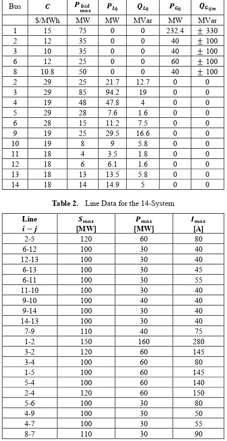
4.1. The 14-Bus Test Case
This section depicts the data set for the IEEE 14-bus test system. Table 1shows supply and demand bids and the bus data for the market participants, whereas Table 2 shows the line data only for 𝑆𝑆𝑚𝑚𝑚𝑚𝑥𝑥, 𝑃𝑃𝑚𝑚𝑚𝑚𝑥𝑥 and 𝐼𝐼𝑚𝑚𝑚𝑚𝑥𝑥. Maximum active power flow limits were computed off-line using a continuation power flow with generation and load directions based on the corresponding power bids, whereas thermal limits were assumed to be twice the values of the line currents at base load conditions for a variation kV voltage rating. In Table 2, it is assumed that 𝐼𝐼𝑖𝑖𝑗𝑗𝑚𝑚𝑚𝑚𝑥𝑥 =𝐼𝐼𝑗𝑗𝑖𝑖𝑚𝑚𝑚𝑚𝑥𝑥 =𝐼𝐼𝑚𝑚𝑚𝑚𝑥𝑥
and 𝑃𝑃𝑖𝑖𝑗𝑗𝑚𝑚𝑚𝑚𝑥𝑥 =𝑃𝑃𝑗𝑗𝑖𝑖𝑚𝑚𝑚𝑚𝑥𝑥 =𝑃𝑃𝑚𝑚𝑚𝑚𝑥𝑥 . Maximum and minimum voltage limits are considered to be 1.1 and 0.9 p.u, so that the results discussed here may also be readily reproduced as presented in[1].
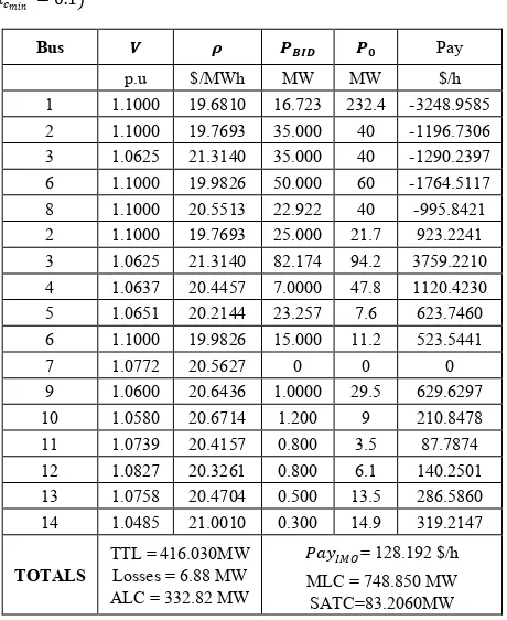
4.2. Results and Discussion
In the following 𝜆𝜆𝑐𝑐 = 0.79999[p.u.] for without and with installing the FACTS devices in Table 3, Table 4, Table 7, Table 8, Table 9, Table 10, Table 11 and Table 12, 𝑉𝑉 is voltage at each bus, 𝜌𝜌 is the LMP, 𝑃𝑃𝐵𝐵𝐼𝐼𝑃𝑃 is supply and demand maximum power bid, 𝑃𝑃0 is generator and load active power including 𝑃𝑃𝐺𝐺0 and 𝑃𝑃𝐿𝐿0, 𝑃𝑃𝑚𝑚𝑦𝑦 is pay for supply and demand. The other definition is the OPF-based approach which represents the maximum load-ability of the network. Furthermore, this value can be viewed as a measure of the congestion of the network, which is represented here using the following maximum loading condition (MLC) definition[19] in case before FACTS installed.
Table 3. OPF with Off-Line Power Flow Limit without FACTS
Bus 𝑽𝑽 𝝆𝝆 𝑷𝑷𝑩𝑩𝑰𝑰𝑩𝑩 𝑷𝑷𝟎𝟎 Pay
p.u. $/MWh MW MW $/h
1 1.1000 17.2997 75.000 232.4 -2720.4677
2 1.0858 17.9112 35.000 40 -1343.3405
3 1.0516 19.2082 35.000 40 -1440.6142
6 1.1000 17.9304 50.000 60 -1972.3493
8 1.1000 18.6447 35.000 40 -1398.3514
2 1.0858 17.9112 25.000 21.7 836.4533
3 1.0516 19.2082 85.000 94.2 3442.1076
4 1.0484 18.5365 48.000 47.8 1775.7970
5 1.0533 18.2142 28.000 7.6 648.4249
6 1.1000 17.9304 15.000 11.2 469.7777
7 1.0601 18.6680 0 0 0
9 1.0352 18.7765 19.302 29.5 916.3357
10 1.0371 18.7666 1.2000 9 191.4192
11 1.0628 18.4309 0.8000 3.5 79.2527
12 1.0809 18.2487 0.8000 6.1 125.9163
13 1.0718 18.4102 0.5000 13.5 257.7432
14 1.0323 19.0239 0.3000 14.9 289.1638
TOTALS TTL = 482.902MW
Losses = 9.353 MW
𝑃𝑃𝑚𝑚𝑦𝑦𝐼𝐼𝐼𝐼𝑃𝑃= 157.2665 $/h
MLC = 531.192 MW SATC = 48.2902 MW
Table 4. VSC-OPF with Off-Line Power Flow Limit with UPFC on
Line-11
Bus 𝑽𝑽 𝝆𝝆 𝑷𝑷𝑩𝑩𝑰𝑰𝑩𝑩 𝑷𝑷𝟎𝟎 Pay
p.u $/MWh MW MW $/h
1 1.1000 17.7226 75.000 232.4 -2776.5839
2 1.1000 17.7947 35.000 40 -1334.6021
3 1.0633 19.1190 35.000 40 -1433.9265
6 1.1000 17.9396 50.000 60 -1973.3595
8 1.1000 18.6413 35.000 40 -1398.0949
2 1.1000 17.7947 25.000 21.7 831.0122
3 1.0633 19.1190 85.000 94.2 3426.1284
4 1.0564 18.5236 48.000 47.8 1774.5585
5 1.0603 18.2416 28.000 7.6 649.4023
6 1.1000 17.9396 15.000 11.2 470.0184
7 1.0632 18.6648 0 0 0
9 1.0376 18.7793 20.616 29.5 941.1352
10 1.0390 18.7708 1.200 9 191.4618
11 1.0638 18.4382 0.800 3.5 79.2843
12 1.0811 18.2570 0.800 6.1 125.9734
13 1.0722 18.4188 0.500 13.5 257.8638
14 1.0338 19.0284 0.300 14.9 289.2323
TOTALS TTL = 484.215MW
Losses = 7.454 MW
𝑃𝑃𝑚𝑚𝑦𝑦𝐼𝐼𝐼𝐼𝑃𝑃= 119.5012 $/h
MLC = 593.360 MW SATC = 109.144 MW
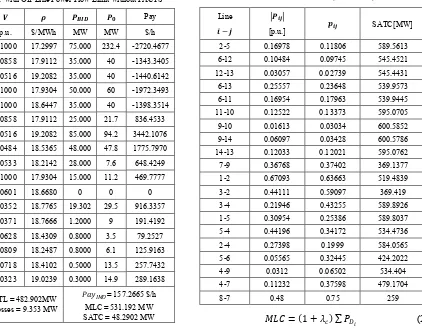
Table 5. Sensitivity Coefficients 𝑝𝑝𝑖𝑖𝑗𝑗 and SATC Determined Applying an N-1 Contingency Criterion without FACTS�𝜆𝜆𝑐𝑐𝑚𝑚𝑖𝑖𝑖𝑖 = 0.1�
Line
𝒃𝒃 − 𝒊𝒊
�𝑷𝑷𝒃𝒃𝒊𝒊�
[p.u.] 𝒑𝒑𝒃𝒃𝒊𝒊 SATC[MW]
2-5 0.16978 0.11806 589.5613
6-12 0.10484 0.09745 545.4521
12-13 0.03057 0.02739 545.4431
6-13 0.25557 0.23648 539.9573
6-11 0.16954 0.17963 539.9445
11-10 0.12522 0.13373 595.0705
9-10 0.01613 0.03034 600.5852
9-14 0.06097 0.03428 600.5786
14-13 0.12033 0.12021 595.0762
7-9 0.36768 0.37402 369.1377
1-2 0.67093 0.63663 519.4839
3-2 0.44111 0.59097 369.419
3-4 0.21946 0.43255 589.8926
1-5 0.30954 0.25386 589.8037
5-4 0.44196 0.34172 534.4736
2-4 0.27398 0.1999 584.0565
5-6 0.05565 0.32445 424.2022
4-9 0.0312 0.06502 534.404
4-7 0.11232 0.37598 479.1704
8-7 0.48 0.75 259
𝐼𝐼𝐿𝐿𝑆𝑆= (1 +𝜆𝜆𝑐𝑐)∑ 𝑃𝑃𝑃𝑃
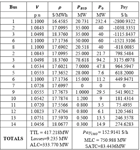
Table 3 depicts the solution of equation (7), showing a low total transaction level (TTL) and the lowest SATC with respect to the maximum power limits of all bids, while as in case[1] the heterogeneous LMPs and NCPs also indicating that system constraints and in particular active power flow limits negatively affect the market solution, however can be corrected by applying FACTS. The SATC value, which was computed off-line with the continuation power flow, seems to be consistent with the chosen power flow limits. Table 3 depicts also the total losses and the payment given to the independent market operator, which is computed as the difference between demand and supply payments[1] as follows:
PayIMO =∑ 𝑆𝑆𝑖𝑖 𝑆𝑆𝑖𝑖𝑃𝑃𝐺𝐺𝑖𝑖− ∑ 𝑆𝑆𝑖𝑖 𝑃𝑃𝑖𝑖𝑃𝑃𝐿𝐿𝑖𝑖 (29) Table 4 depicts the results were be improved with allocated the UPFC in Line-11. The TTL, maximum loading condition (MLC), SATC, LMPs and voltages enhanced, while the total losses and PayIMO given an enhancement.
Table 6. Sensitivity Coefficients 𝑝𝑝𝑖𝑖𝑗𝑗 Determined Applying an N-1
Table 5 shows the coefficients 𝑝𝑝𝑖𝑖𝑗𝑗 used for the sensitivity analysis and the SATCs computed by means of the continuation power flows technique for the two steps required by the iterative method described in Section 3.6.1 when applying the 𝑁𝑁 −1 contingency criterion without installing the FACTS. Observe that both methods lead to similar conclusions, i.e. the sensitivity analysis indicates that the line 1-2 (Line-11) has the highest impact in the system power flows, therefore Line-11 becomes the best location of the FACTS devices, furthermore the 𝑁𝑁 −1 contingency criteria show that the outage of line 1-2 leads to low SATC
Table 6 shows the coefficients 𝑝𝑝𝑖𝑖𝑗𝑗 used for the sensitivity analysis when applying the 𝑁𝑁 −1 contingency criterion which becomes decrease after installing the UPFC in line 1-2.
Table 10. VSC-OPF with Contingency on Line 1-5 with UPFC on Line-11
�𝜆𝜆𝑐𝑐𝑚𝑚𝑖𝑖𝑖𝑖 = 0.1�
Table 7, Table 8 and Table 9 as the following depict the VSC-OPF results for the critical line 1-5, line 2-4 and line 3-2 outage. This solution presents practically the same total transaction level as provided by the solution without contingencies in Table 3, but with different demand side bidding, and a higher SATC, as expected, since the system is now optimized for the given critical contingency. The rescheduling of demand bids results in slightly lower LMPs and NCPs, as a consequence of including more precise security constraints, which is also better results after installing the FACTS devices as seen in Table 10, Table 11 and Table 12 as the following, which in turn results in a lower PayIMO value with respect to the one obtained with
the standard OPF problem equation (7) in Table 3(the higher losses are due the transaction level being higher). Furthermore Table 13 gives NCPs values about the topics that given in Table 3 until Table 12.
Table 11. VSC-OPF with Contingency on Line 2-4 with UPFC on Line-11
�𝜆𝜆𝑐𝑐𝑚𝑚𝑖𝑖𝑖𝑖 = 0.1�
Figure 2 shows the system quiet stable after installing the UPFC on the Line-11 and gives the improvement for some parameter of the electricity base market.
stability margins lead to less congested, i.e. lower, and “cheaper” optimal solutions. For the sake of comparison, Table 10, Table 11 and Table 12 depict the final solution obtained with allocating the UPFC in Line-11. In this case the whole results given satisfactory an enhancement or improvement.
Table 12. VSC-OPF with Contingency on Line 3-2 with UPFC on Line-11
�𝜆𝜆𝑐𝑐𝑚𝑚𝑖𝑖𝑖𝑖 = 0.1�
Table 13. Nodal Congestion Prices Value ($/MWh)
Bus Table
Table 14. Nodal Congestion Prices Value ($/MWh) for System with UPFC
on Line-11
Figure 2. Eigenvalue the IEEE 14-bus system with UPFC on line-11.
Statistics of Eigenvalue: Positive eigs: 0; Negative eigs: 27; Complex pairs: 6; Zero eigs: 0; Dynamic order: 27
Finally, the found of a good system response for the allocated the FACTS devices indicates that the FACTS devices given a good response for the VSC-OPF method with presenting the security method (i.e., V "security" limits) and transaction method (i.e., power transfer limits) in equations (7), (19) and (26) which have the relationship to equation (1) and equation UPFC in Figure 2 for especially voltage, reactance and phase angle between the two terminal voltages.
5. Conclusions
The VSC-OPF based market enhancement are modified and tested on the IEEE 14-Bus test system. The results obtained with VSC-OPF based market including contingencies with installing the FACTS devices techniques and those obtained by means of the VSC-OPF based market including contingencies model only indicate that a proper representation of system security and a proper inclusion of
contingencies with installing the FACTS devices, by using an allocation method, for the two result in improved transactions, higher security margins and lower prices.
The first method gave definition of the worst-case contingency by determining the lowest SATC with the off-line power flow limit without the FACTS as shown in Table 3 that can be improved with the FACTS as shown in Table 4, while the second approach computes sensitivity factors as indicated in Table 5 and Table 6 whose magnitude indicate which line outages and controlling of the FACTS devices maximally affect the system security and total transaction level as indicated in Table 7 until Table 12.
In the relationship with voltage, reactance and phase angle between the two terminal voltages on a transmission line, that is found a good system response for the allocated the FACTS devices which indicates that the FACTS devices given a powerful response for the VSC-OPF method with presenting the security method (i.e., voltage V "security" limits) and the transaction method (i.e., power transfer limits).
Further research work will concentrate in enhancement the OPF techniques performance with modifying of the model and control and then select the best variety and location of the FACTS devices.
ACKNOWLEDGEMENTS
The authors would like to thank for the support and helpful comments of academicals members Gadjah Mada University for this work.
REFERENCES
[1] F. Milano, C. A. Cañizares, M. Invernizzi, “Voltage Stability Constrained OPF Market Models Considering N-1 Contingency Criteria,” Elsevier, Electric Power Systems Research, Vol. 74, No. 1, pp. 27-36, April 2005.
[2] M. Huneault, F.D. Galiana, “A survey of the optimal power flow literature,” IEEE Trans. Power Syst., Vol. 6, No.2, pp. 762–770, 1991.
[3] G.D. Irisarri, X. Wang, J. Tong, S. Mokhtari, “Maximum loadabilityof power systems using interior point nonlinear optimization method,” IEEE Trans. Power Syst., Vol.12, No. 1, pp. 162–172, 1997.
[4] M. Madrigal, “Optimization model and techniques for implementation and pricing of electricity markets,” Ph.D. thesis, University ofWaterloo, Waterloo, Ont., Canada, 2000. [5] V.C. Ramesh, X. Li, “A fuzzy multiobjective approach to
contingency constrained OPF,” IEEE Trans. Power Syst., Vol. 12, No. 3, pp. 1348–1354, 1997.
[6] El-Araby, E.E., Yorino, N., Sasaki, H. and Sugihara, H., A hybrid genetic algorithm/SLP for voltage stability constrained VAR planning problem, Proceedings of the Bulk Power systems Dynamics and Control-V, Onomichi, Japan,
2001.
[7] H. Chen, “Security cost analysis in electricity markets based on voltage security criteria and web-based implementation,” Ph.D. thesis, University of Waterloo, Waterloo, ON, Canada, 2002.
[8] R. Zárate-Miñano, A. J. Conejo, F. Milano, “OPF-Based Security Redispatching Including FACTS Devices,” IET Generation, Transmission & Distribution, Vol. 2, No. 6, pp. 821-833, November 2008.
[9] R. Zárate-Miñano, T. Van Cutsem, F. Milano, A. J. Conejo, “Securing Transient Stability using Time-Domain Simulations within an Optimal Power Flow,” IEEE Transactions on Power Systems, Vol. 25, No. 1, pp. 243-253, February 2010.
[10] R. Zárate-Miñano, F. Milano, A. J. Conejo, “An OPF Methodology to Ensure Small-Signal Stability,” IEEE Transactions on Power Systems, Vol. 26, No. 3, pp. 1050-1061, Aug. 2011.
[11] Canizares, C.A., Chen, H., and Rosehart, W. , Pricing system security in electricity markets, Proceedings of the Bulk Power Systems Dynamics and Control-V, Onomichi, Japan, 2001. [12] F. Milano, “Power System Analysis Toolbox,”
Documentation for PSAT version 2.0.0, February 14, 2008, pp. 194-198.
[13] M. Norozian, L. Angquist, M. Ghandhari and G. Andersson, “Use of UPFC for Optimal Power Flow Control,” IEEE Trans. Power Delivery, vol. 12, no. 4, pp.1629-1634, 1997.
[14] K. Xie, Y.-H. Song, J. Stonham, E. Yu, G. Liu, “Decomposition model and interior point methods for optimal spot pricing of electricity in deregulation environments,” IEEE Trans. Power Syst., Vol.15, No. 1, pp. 39–50, 2000. [15] Gisin, B.S., Obessis, M.V., and Mitsche, J.V., Practical
methods for transfer limit analysis in the power industry deregulated environment, Proceedings of the PICA IEEE International Conference, 1999, pp. 261–266.
[16] F. Milano, C.A. Ca˜nizares, M. Invernizzi, “Multi-objective optimizationfor pricing system security in electricity markets,” IEEE Trans. Power Syst., Vol. 18, No. 2, pp. 596–604, 2003. [17] Available transfer capability definition and determination,
Technical Report, NERC, USA, 1996.
[18] C.A. Ca˜nizares, Z.T. Faur, “Analysis of SVC and TCSC controllers in voltage collapse,” IEEE Trans. Power Syst., Vol. 14, No.1, pp.158–165, 1999.
[19] F. Milano, “Pricing System Security in Electricity Market Models with Inclusion of Voltage Stability Constraints”, Ph.D. Thesis, Electrical Engineering, University of Genova, Genova, Italy, 2003.
[20] V.H. Quintana, G.L. Torres, “Introduction to interior-point methods,” IEEE PICA, Santa Clara, CA, 1999.
[21] MA. Natick. (2012) MATLAB Programming Fundamentals, The MathWorks, Inc., USA,[Online]. Available:http://www. mathworks.com.
[23] M. Ghandhari, “Development of Sensitivity Based Indices for Optimal Placement of UPFC to Minimize Load Curtailment Requirements”, Master Thesis KTH Vetenskap Och Konst, XR-EE-ES-2009:006, 2009.
[24] Saadat, H., 1999, Power System Analysis, WCB/McGraw- Hill Book Co, Singapore.