Three Dimensional Tomography Based on Microearthquake Data at Brady’s Hot Spring Geothermal Field, Nevada

10 - 12 August 2016, Cendrawasih Hall - Jakarta Convention Center, Indonesia

Three Dimensional Tomography Based on Microearthquake Data at Brady’s Hot Spring

Geothermal Field, Nevada

Nanda Hanyfa Maulida, Ahmad Zaenudin, Syamsurijal Rasimeng, Suharno

Geophysical Engineering, University of Lampung nandahanyfa@gmail.com

Keywords: tomography, microearthquake, geothermal,

Brady’s Hot Spring

ABSTRACT

Microearthquake activity in the geothermal field is related to reservoir and sub-surface structure. According to the data recorded, Brady’s Hot Spring which is a non-magmatic convection-dominated geothermal play system has high seismicity. Three-dimensional Vp anomaly, Vs anomaly, and

Vp/Vs-ratio structure are presented for The Brady’s Hot Spring geothermal field using microearthquake travel-time data. The data were recorded by the Northern California Earthquake Data Center (NCEDC) using 8 stations seismic network. In addition, it uses 1D velocity models data and coordinates of the station as supporting data. The data proceed by Lotos 13 consists of determining preliminary location, relocating microearthquake source and inverting tomography by LSQR iterative method, then visualizing the model. The results indicate high Vp anomaly (5% to 25%) and low Vs

anomaly (0% to -15%) in high seismicity zone. It also indicates high Vp/Vs (1.8 to 2.3) in the central section of The Brady’s around high seismicity zone and low Vp/Vs (1.4 to 1.7) below manifestation zone. High and low Vp/Vs-ratios are related to water and steam saturated zones, respectively. Interpretation shows that the reservoir area has high seismicity between 300 to 1400 meters depth, high permeability, and Brady’s Hot Spring main reservoir is in water dominated. As it seen in the result, with tomography inversion we succeed to get very detail seismicity and anomaly velocity distribution related to the reservoir in Brady’s Hot Spring, Nevada.

I. INTRODUCTION

In the geothermal system, there are components must be fulfilled to make complete geothermal system. Those components are a heat source, reservoir rock, structure (fault or fracture), discharge area, cap rock, and fluids. Inexistent of one of that component won’t make perfect the geothermal system. In most of the geothermal reservoir, the fluid moves through the cracks of rocks, or in other words, the rock permeability is controlled by fracture or faults (Philipp et al., 2007). So that in the geothermal field, especially in Brady’s Hot Spring which the main controller of the geothermal system is structure, determine the condition and structure of the subsurface geology became a very important thing to be able to maximize production from geothermal.

Local events from microearthquakes can provide useful information about the geothermal area (Foulger, 1982). It very related to faulting activity, production and injection activity, and also reservoir condition in the field. With the events distribution we can find the main fault in the system which plays an important role in the geothermal system, and by inverting it to the tomography we can clearly see the sub-surface character based on velocity anomaly.

The purposes of this study are to determine the main fault from events distribution, create 3D velocity anomaly tomography and analyze subsurface character based on velocity anomaly tomography in Brady’s Hot Spring geothermal field. Tomography from microearthquake is getting by processing time travel data from every event recorded with inversion method used in the LOTOS.

II. GEOLOGICAL SETTING

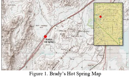
Brady’s Hot Spring Geothermal Field is located in the northern hot spring mountains, about 32 km northeast of Fernley, Nevada. Administratively, this field is in Brady-Hazen, Churchill County, Nevada (Ettinger and Brugman, 1992) 39.80 North and 119 West (Figure 1). This field is using the combination of dual flash power generation, and binary with total installed capacity 26 MWe (Faulds et al., 2010).

Figure 1. Brady’s Hot Spring Map

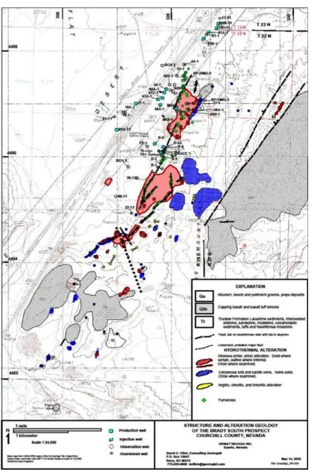
Brady's Hot Springs is located in west-central Nevada in the Basin and Range physiographic province. The surrounding mountains; i.e. Hot Springs Mountains to the south and east, Trinity Range to the north, and Truckee Range to the west form part of the northwestern boundary of the Carson Sink depression. Based on existing data, west-central Nevada was the site of the deposition of eugeosynclinal rocks during the Paleozoic Era. Late Paleozoic Orogenic rock disrupted and telescoped these rocks eastward, but detailed documentation of these effects is meager because post-Paleozoic rocks cover the region. Four stratigraphic units outcrop in Brady's area. An additional three stratigraphic units have been penetrated by the existing wells at Brady's. From the youngest to oldest, these units are alluvium, late Pliocene basalt vents, Truckee formation, Desert Peak formation, Chloropagus formation, an unnamed rhyolite, and basement.

Proceedings The 4th _{Indonesia International Geothermal Convention & Exhibition 2016} 10 - 12 August 2016, Cendrawasih Hall - Jakarta Convention Center, Indonesia (Fauld et al., 2010). Geysers and hot springs have also been

found in this field as well as the reported high surface temperatures and fumaroles (Mesquite Group, Inc., 1997). In addition to thermal manifestations, several other indications of geothermal activity occur along the Brady's Fault Zone. Abundant opaline sinter that commonly cements brecciated rock is found along the fault trace. Small concentrations of cinnabar (mercury sulfide) and native sulfur are present. Intensely hydrothermally altered alluvium occurs in the fault. This material exists as a red, soft, iron-stained kaolinite or a red, silica-cemented kaolinite. Calcite (calcium carbonate) veins containing large euhedral crystals trend along the east side of the fault zone (Mesquite Group, Inc., 1997).

.

Figure 2. Wells, faults, and manifestations location (Lutz et al., 2011)

Based on Moeck (2014) classification, the geothermal system in Brady’s Hot Spring is extensional domain play type which the mantle is elevated due to crustal extension and thinning. The elevated mantle provides the principal source of heat for geothermal systems associated with this play type. The resulting high thermal gradients facilitate the heating of meteoric water circulating through deep faults or permeable formations. Hot Springs Mountains on the northwest and Hot Springs Flat basin on the southeast is the main controlling fault zone in Brady’s geothermal field. The Brady’s area is dominated by NNE-trending gently to moderately tilted fault blocks bounded by moderately to steeply dipping normal faults NNE-trending zone (Faulds et al., 2010).

Figure 3. Faults structure from Brady’s field to Desert Peak (Faulds et al., 2010)

Brady’s system occupy left steps in the NNE-striking, west-dipping normal fault systems. The left steps appear to be linked by multiple minor, more northerly striking faults and thus mark steeply plunging conduits of highly fractured rock. The high fracture density in these steps enhances permeability and therefore accommodates the ascent of hydrothermal fluids (Faulds et al., 2010).

Brady’s Hot Spring geothermal field has a reservoir temperature of 180-193˚C which is a high enthalpy category (Faulds et al., 2010) at 1-2 km depth (Benoit et al., 1982). The Caprock is about 600 meters depth with hydrothermal alteration which has lithology of volcanic hydrothermal alteration in tertiary age. The main rock is a metamorphic basement in Mesozoic age (Lutz et al., 2011). Ettinger and Brugman (1992) mentions that the geothermal field production wells on Brady's cut the production zone at 1000 to 1400 ft (300-425 meters) depth.

III. DATA AND METHOD A. Data Description

The microearthquake data were recorded by the Northern California Earthquake Data Center (NCEDC) using 8 Short-period 3C geophones deployed at the surface (4.5 Hz OYO GS 11-D) since November 2010 to March 2015. For the input data to the LOTOS, we need the description of events which includes hypocenter coordinates, the number of recorded phases, travel time in every phase of the event, geographical coordinates of stations, 1-D starting velocity model, and field topography. 1-D preliminary velocity model dataset is taken from Lawrence Livermore National Laboratory (2013). And ASTER GDEM dataset used for topography map.

B. Step-by-step calculations with the LOTOS code 1. 1D-Velocity Optimization

The purpose of this step is estimation of 1D velocity model which can be then used as starting model for 3D tomographic inversion. First of all, we calculate preliminary location in the 1D velocity model using straight line approximation for the rays. In cases of relatively small size of the study area, it performs the preliminary location of sources using a linear approximation of rays. In this case, the travel times (T) is computed as integral along the straight line between the source (i) and receiver (j) shown by the formula below (Um Thurber, 1987).

𝑇 = ∫

_𝑗𝑖1_𝑣

𝑑𝑙

(1)

where v is wave propagation velocity and dl is ray path segments.

location in the 1D model for events selected in the previous step, and calculation of the first derivative matrix. The matrix is computed along the rays traced in 1D model derived in the previous iteration.

𝑯𝒊𝒋= 𝜕𝑡𝑖/𝜕𝑉𝑗 (2)

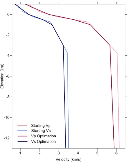
Each element of the matrix is equal to the time deviation (𝜕𝑡) along the ith ray due to a unit-velocity perturbation (𝜕𝑉) in the jth node/block (Koulakov et al., 2006). The depth levels are defined uniformly. Velocity distribution between the levels is approximated linearly. Result of the optimization shown in figure 3.

Figure 3. Results of 1D velocity model optimization 2. Bending Algorithm for Raytracing in a 3D-Velocity

Model

Raytracing algorithm is based on the Fermat principle of traveltime minimization. A basic principle of LOTOS bending algorithm is shown in Figure 3. Searching a path with minimum travel time is performed in several steps. The starting ray path is a straight line (upper plot, green line). In the first step, the ends of the rays are fixed (A and B). This path is deformed in the middle point (line 1). Deformation of the ray path is performed perpendicular to the ray path in two directions: in and across the plane of the ray. The obtained path for the first iteration is shown in the upper plot with a red line.

Then we perform the similar procedure for two segments starting from the path derived in the previous step (red line in middle plot). The resulting path is shown with a blue line. The same procedure is repeated for three (violet line in lower plot) and more segments, and it stops when we reach minimum length of segments. The ray constructed in this way tends to travel through high-velocity anomalies and avoids low-velocity patterns. It should be noted that although a 2D model is shown in Figure 3, the algorithm is designed for the 3D case.

Figure 4. Principle of the bending algorithm for the ray tracing (Koulakov, 2012)

3. Iterative Tomographic Inversion

The starting 1D-velocity model and initial locations of sources are obtained in the step of 1D-model optimization. The sources are then relocated using a code based on 3D raytracing (bending). It then uses gradient method to locate sources in 3D models, which is much faster than another method. The 3D velocity anomalies are computed in nodes distributed in the study volume. Velocity distribution between the nodes is interpolated linearly using subdivision of the study volume into tetrahedral blocks. The nodes are based on vertical lines distributed regularly in map view. In each vertical line, the nodes are installed according to the ray distribution. In the absence of rays, no nodes are installed. In order to reduce the effect of node/cell distributions on the results, we perform the inversion using several grids with different basic orientations (e.g., 0°, 22°, 45°, and 67°). After computing the results for grids with different orientations, they are stacked into one summary model, reducing any artifacts related to grid orientation.

The first derivative matrix is calculated using the ray paths computed after the source locations in the 3D model. Matrix calculation is computed by the bending method. The effect of velocity variation at each node on the traveltime of each ray (𝜕𝑡_𝑖/𝜕𝑣_𝑗) is computed numerically. The data vector corresponding to this matrix consists of residuals obtained after the step of source location.

Inversion is performed simultaneously for P and S velocity anomalies, source parameters (dx, dy, dz, and dt) and P and S station corrections. The system of linear equations has the following structure (Koulakov et al., 2007):

(𝜕𝑡𝑖

𝜕𝑉𝑗𝑃𝑑𝑉𝑗

𝑃_{) + 0 + (𝑊}𝑆𝑐𝑟𝑒 𝜕𝑡𝑖

𝜕𝜎𝑘𝑑𝜎𝑘) + (𝑊

𝑆𝑡_𝑃_𝑑𝜏

𝑠𝑡𝑃) + 0 = 𝑑𝑡𝑖𝑃

(3a)

0 + (𝜕𝑡𝑖

𝜕𝑉𝑗𝑆𝑑𝑉𝑗

𝑆_{) + (𝑊}𝑆𝑐𝑟𝑒 𝜕𝑡𝑖

𝜕𝜎𝑘𝑑𝜎𝑘) + 0 + (𝑊

𝑆𝑡_𝑆_𝑑𝜏

𝑠𝑡𝑆) = 𝑑𝑡𝑖𝑆

(3b)

Proceedings The 4th _{Indonesia International Geothermal Convention & Exhibition 2016} 10 - 12 August 2016, Cendrawasih Hall - Jakarta Convention Center, Indonesia 0 + [𝑆𝑚_𝑆 (𝑑𝑉𝑚𝑆− 𝑑𝑉𝑛𝑆)] + 0 + 0 + 0 = 0 (3d)

(𝑅𝑒_𝑃 𝑑𝑉𝑗𝑃) + 0 + 0 + 0 + 0 = 0 (3e)

0 + (𝑅𝑒_𝑆 𝑑𝑉𝑗𝑆) + 0 + 0 + 0 = 0 (3f)

Here each equation contains five groups corresponding to different unknown parameters. The first and second terms correspond to parameters of P and S velocity anomalies (dVp, dVs). The third term is for corrections of source parameters, 𝜎, which contain source coordinates and origin time. 𝑊𝑆𝑐𝑟𝑒 is a weight for controlling the source parameters. The fourth and fifth terms are for determination of P and S station corrections, 𝑑𝜏_𝑠𝑡𝑃 and 𝑑𝜏_𝑠𝑡𝑆. 𝑊𝑆𝑡_𝑃 and 𝑊𝑆𝑡_𝑆are the weights for the P and S station corrections.

Equations (3a) and (3b) are the main equations with the observed residuals, dtP _{and dt}S_{, in the right part. The other} equations are supplementary ones for controlling smoothness and amplitude of the velocity models. Equations (3c) and (3d) each contain two nonzero elements with opposite signs, corresponding to neighboring parameterization nodes in the model (with indexes m and n). The data vector corresponding to this block is zero. Increasing the weight of these elements, Sm_P and Sm_S, has a flattening effect upon the resulting anomalies. The block which controls the amplitude of the model (equations (3e) and (3f)) has a diagonal structure with only one element in each equation and zero values in the data vector. Re_P and Re_S are the coefficients for the amplitude adjustment (regularization parameters).

The steps of grid construction, matrix calculation, and inversion are performed for several grids with different basic orientations. The resulting velocity anomalies derived for all grids are combined and computed in a regular grid. This model is added to the absolute-velocity distributions used in a previous iteration. New iterations repeat the steps of source location, matrix calculation, and inversion. After performing the inversions for several grids with different orientations, the velocity anomalies are recomputed in a 3D regular grid.

IV. RESULT

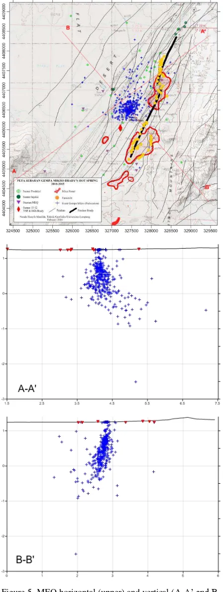
The main structure (fault or fracture) played in the geothermal system can be seen from microearthquake events distribution. The structure is important media to transfer the fluids in or out the reservoir as injecting and producing activity. By the data, horizontal distribution of events in the Brady’s and vertical distribution shown in figure 5. As we see from the surface (upper picture), the distribution of micro earthquakes is concentrated in the west area of Brady’s Fault. And by looking at the data from the 3D distribution of the hypocenter (Figure 6) which overlaid with a model of the fault, the distribution of micro earthquakes still get in on Brady’s Fault area which is the target production with fracture dip according to Jolie et al (2012) about 70˚ - 80˚. Hereby it can be concluded that the cause of the majority of micro earthquakes is due to the activity of reservoir (production and injection) and some activity near the surface of the structure.

Activities structure near the surface are closely associated with the process of deformation of the surface that quite intense in this geothermal field (Davatzes et al., 2013) which can be caused by thermal cooling reservoir gradually or compaction of sediment due to increased pore pressure and desaturation (Ali et al., 2016)

Figure 6. 3D microearthquake hypocenter distribution at Brady's Hot Spring

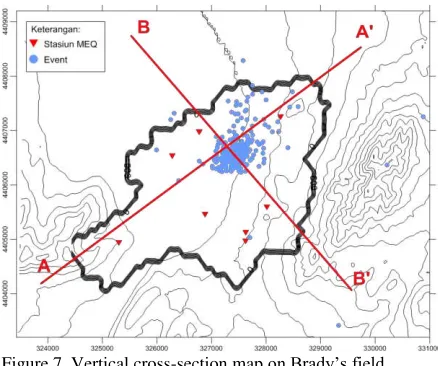
Tomographic inversion performed by LOTOS produce 3D subsurface models from Brady’s field. The model is represented by Vp, Vs, and Vp / Vs spread map anomaly. Vertically, taken two sections, A-A' and B-B' intersecting at the center of the field as shown in Figure 7. A-A' Southwestern - Northeast and direction of cross-section B-B' Northwest - Southeast. 4 cross-section taken horizontally representing elevation 1 km, 0.6 km, 0 km (sea level) and -1 km from the sea surface.

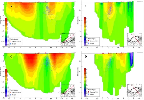
Figure 7. Vertical cross-section map on Brady’s field The value of Vp and Vs anomaly distribution stated in percent change of velocity perturbation to the surrounding layers. Based on the vertical cross section of the P wave tomography anomalies (Figure 8A and B), the microearthquake distribution zone which is expected to be a production zone has a relatively high anomaly ranging from 5% to 25%. In the cross-section B-B', highly anomalous zone centered on the microearthquakes distribution, then becomes low on the right and left cross-section reaches 20%.

Conditions were a little different on the vertical section of the

Vs anomaly tomography (Figure 8C and D), microearthquake distribution zone has relatively low anomalous, 15% slower than the surrounding velocity, and higher in other zones in the cross-section A-A'. In the cross-section B-B', the value of low anomaly seen in the microearthquakes distribution zone and slightly lower in the zone on the right of the cross-section, more than -25%.

By looking at the horizontal cross-section it can be seen a clearer lateral velocity anomaly distribution on Brady Field. The cross-section is divided into four sections. The top section in the 1000 meters above sea level or at approximately 200-250 meters depth from the surface. The second section in the 600 meters above sea level, then section at the sea level (0 meters), and 1000 meters below sea level. As seen in vertical cross-section, the distribution of high P wave anomaly spread in the microearthquakes distribution zone along the Southwestern 5% to 25% (Figure 9). This high anomaly decreased with increasing depth. While the other zones in the negative anomaly find wide enough to more than minus 25% with the lowest in the Southeast region.

If the anomalous distribution of the P wave is dominated by low anomaly at low seismicity zone, otherwise the anomalous distribution of S wave is dominated by high anomaly (10% to 50%). At a 1000 meters elevation (200-250 meters depth), high anomaly relative aft direction with Southwestern-Northeast (Figure 10), as well as at 600 meters elevation (600-650 meters depth) but with the diminishing area. High seismicity zone is dominated by the low S wave anomalies were 0 up to -15% and rising with increasing depth. If we see the comparison between the P and S waves anomalies at the line A-A' (Figure 8A and C), it provides a different distribution information anomalies. A-A' is a path along the Southwestern - Northeast that tends to follow the trend or direction of the fault on the field Brady but still cut the faults. At the high seismicity zone, it obtained high P wave anomaly and low S wave anomaly. This condition indicates a high water saturation as stated by Wang (1990). Changes in temperature which isn’t too significant (stable) are not disturbing wave velocity so that the effect of temperature is not too visible.

On the left zone of the section also encountered anomalous high P and low S anomaly identical as in high seismicity zone, but also demonstrated high S anomalies near the middle zone. If it is associated with structural geology, zones with high P and S anomaly correlated with the less fracture area. Then the condition with this high anomaly is identified due to the high density in the area.

Proceedings The 4th _{Indonesia International Geothermal Convention & Exhibition 2016} 10 - 12 August 2016, Cendrawasih Hall - Jakarta Convention Center, Indonesia

Figure 8. Vertical cross-section P wave anomalies tomography (in percent) at line A-A' (A) and B-B' (B) and S wave anomaly

tomography at line A-A’ (C) and B-B’ (D)

Figure 9. Horizontal cross-section P wave anomalies tomography (in percent) at 1, 0.6, 0 and -1 km from sea level

Figure 10. Horizontal cross-section S wave anomalies tomography (in percent) at 1, 0.6, 0 and -1 km from sea level

A B

10 - 12 August 2016, Cendrawasih Hall - Jakarta Convention Center, Indonesia Besides Vp and Vs anomalies, the inversion also generates the

Vp/Vs distribution (Figure 11). Comparison of Vp/Vs obtained from the results of this inversion has a value range 1.5 to 2.3. In Figure 11, the high seismicity zone is dominated by the high Vp / Vs, which is one characteristic of the geothermal field. This high ratio spread only to approximately 1500 meters depth, then getting lower both in the cross sections A-A’and B-B’ at a greater depth. If the cross sections Vp/Vs

tomographic compared with the Vp and Vs anomaly distribution shown before (Figure 8), it can be seen that although the eastern part of the cross sections A-A' have the

low Vp anomaly and high Vs anomaly, the Vp/Vs ratio were obtained low.

Horizontally can be seen that Vp/Vs has a high ratio of a value close to 2, centered on the high seismicity zone and extends toward Southwestern decreasing with increasing depth (Figure 12). While the Northeast region is dominated by the value of the low Vp/Vs ratio. Vp/Vs is also known as Poisson coefficient and can be used to determine the subsurface fluid condition.

Figure 11. Vertical cross-section Vp/Vs tomographi line A-A’ and B-B’

Figure 12. Horizontal cross-section Vp/Vs tomography at 1, 0.6, 0 and -1 km from sea level The ratio of Vp/Vs is used as a parameter to determine the

condition of the fluid under the surface. In theory, the relationship between Vp/Vs and water saturation states that the higher Vp/Vs value, the water saturation also higher. The anomalous values Vp/Vs high value often associated with cracks in the rocks that filled the fluid. Vp/Vs interpreted the low value associated with the dry rock and filled gas or steam (Mashuri, 2015).

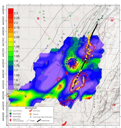
By creating an overlay between Vp/Vs tomography at 600 meters elevation (600-650 meters depth) and with surface geothermal manifestations (Figure 13), it is known that the low Vp/Vs spread under Fumarole and sinter manifestations, which defines as the steam below the surface manifestations. Most of the microearthquake events are covered in the high

Vp/Vs zone and are assumed to be Brady’s Field main reservoir with high water saturation. Some events occur outside of the reservoir and is assumed to occur due to the re-injection or replenishment process natural subsurface water of the surface water seepage.

As said by Thurber et al. (1997), that the association between the zones with high Vp/Vs and high seismicity indicate the direct involvement of the fluid in the process of faults/fracture. Also seen in Figure 13 the potential reservoir occur in the Southwestern region, but because of there’s not enough faults and permeability structure which are

characterized by low seismicity, it becomes hard to develope the production in the area.

Proceedings The 4th _{Indonesia International Geothermal Convention & Exhibition 2016} 10 - 12 August 2016, Cendrawasih Hall - Jakarta Convention Center, Indonesia V. CONCLUSION

By the result that described above, we can conclude that the main structure played as the production zone in the Brady’s Hot Spring field is Brady’s fault which dip about 70˚-80˚ proofed by high seismicity distribution that located in the western of Brady’s faults area with similar dip as the fault. This production zone has high P-wave velocity anomaly by 5% to 25% and the low Swave velocity anomaly by 0% to -15% that shown high density but with fluid content in it. The value of Vp/Vs which shows 1.8 to 2.3 make clear that the fluid content is water. So the Brady’s Hot Spring main reservoir is in Brady’s fault area and in water dominated system.

VI. ACKNOWLEDGEMENT

We thank Mr Ivan Koulakov who assist and help us to solve the problem when using LOTOS. We would also like to show our gratitude to the NCEDC, NASA and METI and all organization that provide the data for free. Waveform data, metadata, or data products for this study were accessed through the Northern California Earthquake Data Center (NCEDC), doi:10.7932/NCEDC. ASTER GDEM is a product of METI and NASA

VII.REFFERENCES

Ali, S. T., et al. (2016). Time-series analysis of surface deformation at Brady Hot Springs geothermal field (Nevada) using interferometric synthetic aperture radar.

Geothermics, 61. pp.114-120.

Benoit, W. R., et al. (1982). Discovery and geology of the Desert Peak Geothermal Field: A case history. University of Nevada.

Davatzes, N. C., et al. (2013, February). Preliminary investigation of reservoir dynamics monitored through combined surface deformation and micro-earthquake activity: Brady’s geothermal field, Nevada. In Proceedings of the Thirty-Eighth Workshop on Geothermal Reservoir Engineering, Stanford, California (pp. 11-13).

Ettinger, T., & Brugman, J. (1992). Brady Hot Springs geothermal power plant.Geothermal Res. Council Bull, 21(8), 258-260.

Faulds, J. E., et al. (2010). Structural controls of geothermal activity in the northern Hot Springs Mountains, western Nevada: The tale of three geothermal systems (Brady’s, Desert Peak, and Desert Queen). Geothermal Resources Council Transactions, 34, 675-683.

Foulger, G. (1982). Geothermal exploration and reservoir monitoring using earthquakes and the passive seismic method. Geothermics, 11(4), 259-268.

Jolie, E., et al. (2012). The Development of a 3D Structural-Geological Model as Part of The Geothermal Exploration Strategy–A Case Study From the Brady’s Geothermal System, Nevada, USA. Proceedings, 37th Workshop on Geothermal Reservoir Engineering. Stanford University, Stanford, California, January 30-February 1.

Koulakov, I., et al. (2006). P-and S-velocity images of the lithosphere—asthenosphere system in the Central Andes

from local-source tomographic inversion. Geophysical Journal International, 167(1), 106-126.

Koulakov, I., et al. (2007). P and S velocity structure of the crust and the upper mantle beneath central Java from local tomography inversion. J. Geophys. Res. 112:B08310, doi:10.1029/2006JB004712

Koulakov, I. 2009. LOTOS Code for Local Earthquake Tomographic Inversion: Benchmarks For Testing Tomographic Algorithms. Bulletin of the Seismological Society of America. 99(1):194-214.

Lawrence Livermore National Laboratory. (2013). Brady 1D seismic velocity model ambient noise prelim [data set]. Retrieved from http://gdr.openei.org/submissions/262. doi:10.15121/1148801

Lutz, S. J., et al. (2011). Lithologies, hydrothermal alteration, and rock mechanical properties in wells 15-12 and BCH-3, Bradys Hot Springs geothermal field, Nevada. GRC Transactions, 35, 469-476.

Mesquite Group, Inc. (1997). Conceptual Geologic Model For Brady's Geothermal Field, Nevada.

Moeck, I. S. (2014). Catalog of geothermal play types based on geologic controls. Renewable and Sustainable Energy Reviews, 37, 867-882.

NASA & METI. 2011. ASTER Global Digital Elevation Model (GDEM). Version 2. NASA EOSDIS Land Processes DAAC, USGS Earth Resources Observation and Science (EROS) Center, Sioux Falls, South Dakota (https://lpdaac.usgs.gov), accessed July 22, 2016

NCEDC (2014), Northern California Earthquake Data Center. UC Berkeley Seismological Laboratory. Dataset. doi:10.7932/NCEDC.

Philipp, S. L., Gudmundsson, A., & Oelrich, A. R. (2007). How structural geology can contribute to make geothermal projects successful. In Proc. European Geothermal Congress (pp. 1-10).

Thurber, C., & Ritsema, J. (2007). Seismic tomography and inverse methods.Treatise on Geophysics. Oxford: Elsevier, 1, 1323-1360.

Um, J., & Thurber, C. (1987). A fast algorithm for two-point seismic ray tracing.Bulletin of the Seismological Society of America, 77(3), 972-986.

University of Wisconsin. (2014). Brady's Geothermal Field Seismic Network Metadata [data set]. Retrieved from http://gdr.openei.org/submissions/469.

doi:10.15121/1166944