R for Beginners
Emmanuel Paradis
Institut des Sciences de l’ ´Evolution Universit´e Montpellier II F-34095 Montpellier c´edex 05 France
I thank Julien Claude, Christophe Declercq, ´Elodie Gazave, Friedrich Leisch, Louis Luangkesron, Fran¸cois Pinard, and Mathieu Ros for their comments and suggestions on earlier versions of this document. I am also grateful to all the members of the R Development Core Team for their considerable efforts in developing R and animating the discussion list ‘rhelp’. Thanks also to the R users whose questions or comments helped me to write “R for Beginners”. Special thanks to Jorge Ahumada for the Spanish translation.
c
2002, 2005, Emmanuel Paradis (12th September 2005)
Contents
1 Preamble 1
2 A few concepts before starting 3
2.1 How R works . . . 3
2.2 Creating, listing and deleting the objects in memory . . . 5
2.3 The on-line help . . . 7
3 Data with R 9 3.1 Objects . . . 9
3.2 Reading data in a file . . . 11
3.3 Saving data . . . 14
3.4 Generating data . . . 15
3.4.1 Regular sequences . . . 15
3.4.2 Random sequences . . . 17
3.5 Manipulating objects . . . 18
3.5.1 Creating objects . . . 18
3.5.2 Converting objects . . . 23
3.5.3 Operators . . . 25
3.5.4 Accessing the values of an object: the indexing system . 26 3.5.5 Accessing the values of an object with names . . . 29
3.5.6 The data editor . . . 31
3.5.7 Arithmetics and simple functions . . . 31
3.5.8 Matrix computation . . . 33
4 Graphics with R 36 4.1 Managing graphics . . . 36
4.1.1 Opening several graphical devices. . . 36
4.1.2 Partitioning a graphic . . . 37
4.2 Graphical functions. . . 40
4.3 Low-level plotting commands . . . 41
4.4 Graphical parameters . . . 43
4.5 A practical example . . . 44
4.6 Thegrid and latticepackages . . . 48
5 Statistical analyses with R 55 5.1 A simple example of analysis of variance . . . 55
5.2 Formulae . . . 56
5.3 Generic functions . . . 58
6 Programming with R in pratice 64
6.1 Loops and vectorization . . . 64
6.2 Writing a program in R . . . 66
6.3 Writing your own functions . . . 67
1
Preamble
The goal of the present document is to give a starting point for people newly interested in R. I chose to emphasize on the understanding of how R works, with the aim of a beginner, rather than expert, use. Given that the possibilities offered by R are vast, it is useful to a beginner to get some notions and concepts in order to progress easily. I tried to simplify the explanations as much as I could to make them understandable by all, while giving useful details, sometimes with tables.
R is a system for statistical analyses and graphics created by Ross Ihaka and Robert Gentleman1. R is both a software and a language considered as a dialect of the S language created by the AT&T Bell Laboratories. S is available as the software S-PLUS commercialized by Insightful2. There are important differences in the designs of R and of S: those who want to know more on this point can read the paper by Ihaka & Gentleman (1996) or the R-FAQ3, a copy
of which is also distributed with R.
R is freely distributed under the terms of theGNU General Public Licence4; its development and distribution are carried out by several statisticians known as theR Development Core Team.
R is available in several forms: the sources (written mainly in C and some routines in Fortran), essentially for Unix and Linux machines, or some pre-compiled binaries for Windows, Linux, and Macintosh. The files needed to install R, either from the sources or from the pre-compiled binaries, are distributed from the internet site of the Comprehensive R Archive Network (CRAN)5 where the instructions for the installation are also available. Re-garding the distributions of Linux (Debian, . . . ), the binaries are generally available for the most recent versions; look at the CRAN site if necessary.
R has many functions for statistical analyses and graphics; the latter are visualized immediately in their own window and can be saved in various for-mats (jpg, png, bmp, ps, pdf, emf, pictex, xfig; the available forfor-mats may depend on the operating system). The results from a statistical analysis are displayed on the screen, some intermediate results (P-values, regression coef-ficients, residuals, . . . ) can be saved, written in a file, or used in subsequent analyses.
The R language allows the user, for instance, to program loops to suc-cessively analyse several data sets. It is also possible to combine in a single program different statistical functions to perform more complex analyses. The
1
Ihaka R. & Gentleman R. 1996. R: a language for data analysis and graphics. Journal
of Computational and Graphical Statistics5: 299–314. 2
Seehttp://www.insightful.com/products/splus/default.asp for more information 3
http://cran.r-project.org/doc/FAQ/R-FAQ.html
4
For more information: http://www.gnu.org/
5
R users may benefit from a large number of programs written for S and avail-able on the internet6, most of these programs can be used directly with R.
At first, R could seem too complex for a non-specialist. This may not be true actually. In fact, a prominent feature of R is its flexibility. Whereas a classical software displays immediately the results of an analysis, R stores these results in an “object”, so that an analysis can be done with no result displayed. The user may be surprised by this, but such a feature is very useful. Indeed, the user can extract only the part of the results which is of interest. For example, if one runs a series of 20 regressions and wants to compare the different regression coefficients, R can display only the estimated coefficients: thus the results may take a single line, whereas a classical software could well open 20 results windows. We will see other examples illustrating the flexibility of a system such as R compared to traditional softwares.
6
2
A few concepts before starting
Once R is installed on your computer, the software is executed by launching the corresponding executable. The prompt, by default ‘>’, indicates that R is waiting for your commands. Under Windows using the program Rgui.exe, some commands (accessing the on-line help, opening files, . . . ) can be executed via the pull-down menus. At this stage, a new user is likely to wonder “What do I do now?” It is indeed very useful to have a few ideas on how R works when it is used for the first time, and this is what we will see now.
We shall see first briefly how R works. Then, I will describe the “assign” operator which allows creating objects, how to manage objects in memory, and finally how to use the on-line help which is very useful when running R.
2.1 How R works
The fact that R is a language may deter some users who think “I can’t pro-gram”. This should not be the case for two reasons. First, R is an interpreted language, not a compiled one, meaning that all commands typed on the key-board are directly executed without requiring to build a complete program like in most computer languages (C, Fortran, Pascal, . . . ).
Second, R’s syntax is very simple and intuitive. For instance, a linear regression can be done with the command lm(y ~ x) which means “fitting a linear model with y as response and x as predictor”. In R, in order to be executed, a function always needs to be written with parentheses, even if there is nothing within them (e.g., ls()). If one just types the name of a function without parentheses, R will display the content of the function. In this document, the names of the functions are generally written with parentheses in order to distinguish them from other objects, unless the text indicates clearly so.
When R is running, variables, data, functions, results, etc, are stored in the active memory of the computer in the form ofobjects which have aname. The user can do actions on these objects with operators (arithmetic, logical, comparison, . . . ) and functions (which are themselves objects). The use of operators is relatively intuitive, we will see the details later (p. 25). An R function may be sketched as follows:
arguments−→
options−→
function
↑
default arguments
=⇒result
of which could be defined by default in the function; these default values may be modified by the user by specifying options. An R function may require no argument: either all arguments are defined by default (and their values can be modified with the options), or no argument has been defined in the function. We will see later in more details how to use and build functions (p. 67). The present description is sufficient for the moment to understand how R works.
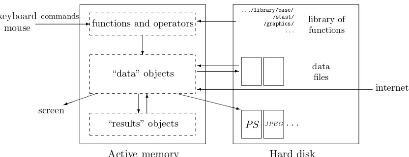
All the actions of R are done on objects stored in the active memory of the computer: no temporary files are used (Fig.1). The readings and writings of files are used for input and output of data and results (graphics, . . . ). The user executes the functions via some commands. The results are displayed directly on the screen, stored in an object, or written on the disk (particularly for graphics). Since the results are themselves objects, they can be considered as data and analysed as such. Data files can be read from the local disk or from a remote server through internet.
functions and operators
❄
“data” objects
❄✻
✏ ✏ ✏ ✏
✮ ❳❳❳❳❳❳❳③
“results” objects
.../library/base/ /stast/ /graphics/ ...
library of functions
✛
data files
✛ ✲
internet
✛
PS JPEG. . .
keyboard
mouse ✲
commands
screen
Active memory Hard disk
Figure 1: A schematic view of how R works.
The functions available to the user are stored in a library localised on the disk in a directory called R HOME/library (R HOME is the directory where R is installed). This directory containspackages of functions, which are themselves structured in directories. The package named baseis in a way the core of R and contains the basic functions of the language, particularly, for reading and manipulating data. Each package has a directory called R with a file named like the package (for instance, for the package base, this is the file R HOME/library/base/R/base). This file contains all the functions of the package.
One of the simplest commands is to type the name of an object to display its content. For instance, if an objectncontents the value 10:
The digit 1 within brackets indicates that the display starts at the first element of n. This command is an implicit use of the function printand the above example is similar toprint(n)(in some situations, the functionprint
must be used explicitly, such as within a function or a loop).
The name of an object must start with a letter (A–Z and a–z) and can include letters, digits (0–9), dots (.), and underscores ( ). R discriminates between uppercase letters and lowercase ones in the names of the objects, so thatxand Xcan name two distinct objects (even under Windows).
2.2 Creating, listing and deleting the objects in memory
An object can be created with the “assign” operator which is written as an arrow with a minus sign and a bracket; this symbol can be oriented left-to-right or the reverse:
> n <- 15 > n
[1] 15 > 5 -> n > n [1] 5 > x <- 1 > X <- 10 > x
[1] 1 > X [1] 10
If the object already exists, its previous value is erased (the modification affects only the objects in the active memory, not the data on the disk). The value assigned this way may be the result of an operation and/or a function:
> n <- 10 + 2 > n
[1] 12
> n <- 3 + rnorm(1) > n
[1] 2.208807
The functionrnorm(1)generates a normal random variate with mean zero and variance unity (p. 17). Note that you can simply type an expression without assigning its value to an object, the result is thus displayed on the screen but is not stored in memory:
The assignment will be omitted in the examples if not necessary for un-derstanding.
The functionls lists simply the objects in memory: only the names of the objects are displayed.
> name <- "Carmen"; n1 <- 10; n2 <- 100; m <- 0.5 > ls()
[1] "m" "n1" "n2" "name"
Note the use of the semi-colon to separate distinct commands on the same line. If we want to list only the objects which contain a given character in their name, the option pattern (which can be abbreviated with pat) can be used:
> ls(pat = "m") [1] "m" "name"
To restrict the list of objects whose names start with this character:
> ls(pat = "^m") [1] "m"
The function ls.strdisplays some details on the objects in memory:
> ls.str() m : num 0.5 n1 : num 10 n2 : num 100
name : chr "Carmen"
The option pattern can be used in the same way as with ls. Another useful option of ls.strismax.levelwhich specifies the level of detail for the display of composite objects. By default, ls.str displays the details of all objects in memory, included the columns of data frames, matrices and lists, which can result in a very long display. We can avoid to display all these details with the option max.level = -1:
> M <- data.frame(n1, n2, m) > ls.str(pat = "M")
M : ‘data.frame’: 1 obs. of 3 variables: $ n1: num 10
$ n2: num 100 $ m : num 0.5
> ls.str(pat="M", max.level=-1)
M : ‘data.frame’: 1 obs. of 3 variables:
2.3 The on-line help
The on-line help of R gives very useful information on how to use the functions. Help is available directly for a given function, for instance:
> ?lm
will display, within R, the help page for the functionlm()(linear model). The commandshelp(lm)andhelp("lm")have the same effect. The last one must be used to access help with non-conventional characters:
> ?*
Error: syntax error > help("*")
Arithmetic package:base R Documentation
Arithmetic Operators ...
Calling help opens a page (this depends on the operating system) with general information on the first line such as the name of the package where is (are) the documented function(s) or operators. Then comes a title followed by sections which give detailed information.
Description: brief description.
Usage: for a function, gives the name with all its arguments and the possible
options (with the corresponding default values); for an operator gives the typical use.
Arguments: for a function, details each of its arguments.
Details: detailed description.
Value: if applicable, the type of object returned by the function or the
oper-ator.
See Also: other help pages close or similar to the present one.
Examples: some examples which can generally be executed without opening
the help with the functionexample.
For beginners, it is good to look at the section Examples. Generally, it is useful to read carefully the section Arguments. Other sections may be encountered, such asNote,References or Author(s).
> help("bs")
No documentation for ’bs’ in specified packages and libraries: you could try ’help.search("bs")’
> help("bs", try.all.packages = TRUE)
Help for topic ’bs’ is not in any loaded package but can be found in the following packages:
Package Library
splines /usr/lib/R/library
Note that in this case the help page of the function bs is not displayed. The user can display help pages from a package not loaded in memory using the option package:
> help("bs", package = "splines")
bs package:splines R Documentation
B-Spline Basis for Polynomial Splines
Description:
Generate the B-spline basis matrix for a polynomial spline. ...
The help in html format (read, e.g., with Netscape) is called by typing:
> help.start()
A search with keywords is possible with this html help. The section See Also has here hypertext links to other function help pages. The search with keywords is also possible in R with the function help.search. The latter looks for a specified topic, given as a character string, in the help pages of all installed packages. For instance, help.search("tree")will display a list of the functions which help pages mention “tree”. Note that if some packages have been recently installed, it may be useful to refresh the database used by
help.searchusing the optionrebuild(e.g.,help.search("tree", rebuild = TRUE)).
The fonctionaproposfinds all functions which name contains the character string given as argument; only the packages loaded in memory are searched:
> apropos(help)
3
Data with R
3.1 Objects
We have seen that R works with objects which are, of course, characterized by their names and their content, but also byattributes which specify the kind of data represented by an object. In order to understand the usefulness of these attributes, consider a variable that takes the value 1, 2, or 3: such a variable could be an integer variable (for instance, the number of eggs in a nest), or the coding of a categorical variable (for instance, sex in some populations of crustaceans: male, female, or hermaphrodite).
It is clear that the statistical analysis of this variable will not be the same in both cases: with R, the attributes of the object give the necessary information. More technically, and more generally, the action of a function on an object depends on the attributes of the latter.
All objects have two intrinsic attributes: mode and length. The mode is the basic type of the elements of the object; there are four main modes: numeric, character, complex7, and logical (FALSEor TRUE). Other modes exist but they do not represent data, for instance function or expression. The length is the number of elements of the object. To display the mode and the length of an object, one can use the functionsmodeand length, respectively:
> x <- 1 > mode(x) [1] "numeric" > length(x) [1] 1
> A <- "Gomphotherium"; compar <- TRUE; z <- 1i > mode(A); mode(compar); mode(z)
[1] "character" [1] "logical" [1] "complex"
Whatever the mode, missing data are represented by NA (not available). A very large numeric value can be specified with an exponential notation:
> N <- 2.1e23 > N
[1] 2.1e+23
R correctly represents non-finite numeric values, such as±∞withInfand
-Inf, or values which are not numbers with NaN(not a number).
7
> x <- 5/0 > x
[1] Inf > exp(x) [1] Inf > exp(-x) [1] 0 > x - x [1] NaN
A value of mode character is input with double quotes ". It is possible to include this latter character in the value if it follows a backslash \. The two charaters altogether\"will be treated in a specific way by some functions such ascatfor display on screen, orwrite.tableto write on the disk (p. 14, the option qmethodof this function).
> x <- "Double quotes \" delimitate R’s strings." > x
[1] "Double quotes \" delimitate R’s strings." > cat(x)
Double quotes " delimitate R’s strings.
Alternatively, variables of mode character can be delimited with single quotes (’); in this case it is not necessary to escape double quotes with back-slashes (but single quotes must be!):
> x <- ’Double quotes " delimitate R\’s strings.’ > x
[1] "Double quotes \" delimitate R’s strings."
The following table gives an overview of the type of objects representing data.
object modes several modes
possible in the same object?
vector numeric, character, complexor logical No
factor numericor character No
array numeric, character, complexor logical No
matrix numeric, character, complexor logical No data frame numeric, character, complexor logical Yes
ts numeric, character, complexor logical No
list numeric, character, complex, logical, Yes
A vector is a variable in the commonly admitted meaning. A factor is a categorical variable. An array is a table with k dimensions, a matrix being a particular case of array with k = 2. Note that the elements of an array or of a matrix are all of the same mode. A data frame is a table composed with one or several vectors and/or factors all of the same length but possibly of different modes. A ‘ts’ is a time series data set and so contains additional attributes such as frequency and dates. Finally, a list can contain any type of object, included lists!
For a vector, its mode and length are sufficient to describe the data. For other objects, other information is necessary and it is given by non-intrinsic attributes. Among these attributes, we can citedim which corresponds to the dimensions of an object. For example, a matrix with 2 lines and 2 columns has fordimthe pair of values [2, 2], but its length is 4.
3.2 Reading data in a file
For reading and writing in files, R uses the working directory. To find this directory, the commandgetwd()(get working directory) can be used, and the working directory can be changed withsetwd("C:/data")or setwd("/home/-paradis/R"). It is necessary to give the path to a file if it is not in the working directory.8
R can read data stored in text (ASCII) files with the following functions:
read.table (which has several variants, see below), scan and read.fwf. R can also read files in other formats (Excel, SAS, SPSS, . . . ), and access SQL-type databases, but the functions needed for this are not in the packagebase. These functionalities are very useful for a more advanced use of R, but we will restrict here to reading files in ASCII format.
The function read.table has for effect to create a data frame, and so is the main way to read data in tabular form. For instance, if one has a file named data.dat, the command:
> mydata <- read.table("data.dat")
will create a data frame namedmydata, and each variable will be named, by de-fault,V1,V2, . . . and can be accessed individually by mydata$V1,mydata$V2, . . . , or by mydata["V1"], mydata["V2"], . . . , or, still another solution, by
mydata[, 1], mydata[,2 ], . . .9 There are several options whose default values (i.e. those used by R if they are omitted by the user) are detailed in the following table:
read.table(file, header = FALSE, sep = "", quote = "\"’", dec = ".",
8
Under Windows, it is useful to create a short-cut of Rgui.exe then edit its properties and change the directory in the field “Start in:” under the tab “Short-cut”: this directory will then be the working directory if R is started from this short-cut.
9
There is a difference: mydata$V1andmydata[, 1]are vectors whereasmydata["V1"]is
row.names, col.names, as.is = FALSE, na.strings = "NA", colClasses = NA, nrows = -1,
skip = 0, check.names = TRUE, fill = !blank.lines.skip, strip.white = FALSE, blank.lines.skip = TRUE,
comment.char = "#")
file the name of the file (within"" or a variable of mode character),
possibly with its path (the symbol\ is not allowed and must be
replaced by /, even under Windows), or a remote access to a file of type URL (http://...)
header a logical (FALSEorTRUE) indicating if the file contains the names of
the variables on its first line
sep the field separator used in the file, for instancesep="\t" if it is a
tabulation
quote the characters used to cite the variables of mode character
dec the character used for the decimal point
row.names a vector with the names of the lines which can be either a vector of
mode character, or the number (or the name) of a variable of the file (by default: 1,2,3, . . . )
col.names a vector with the names of the variables (by default: V1, V2, V3,
. . . )
as.is controls the conversion of character variables as factors (ifFALSE)
or keeps them as characters (TRUE);as.iscan be a logical, numeric
or character vector specifying the variables to be kept as character
na.strings the value given to missing data (converted as NA)
colClasses a vector of mode character giving the classes to attribute to the
columns
nrows the maximum number of lines to read (negative values are ignored)
skip the number of lines to be skipped before reading the data
check.names if TRUE, checks that the variable names are valid for R
fill if TRUE and all lines do not have the same number of variables,
“blanks” are added
strip.white (conditional to sep) if TRUE, deletes extra spaces before and after
the character variables
blank.lines.skip if TRUE, ignores “blank” lines
comment.char a character defining comments in the data file, the rest of the
line after this character is ignored (to disable this argument, use
comment.char = "")
The variants of read.table are useful since they have different default values:
read.csv(file, header = TRUE, sep = ",", quote="\"", dec=".", fill = TRUE, ...)
read.csv2(file, header = TRUE, sep = ";", quote="\"", dec=",", fill = TRUE, ...)
read.delim(file, header = TRUE, sep = "\t", quote="\"", dec=".", fill = TRUE, ...)
The function scan is more flexible thanread.table. A difference is that it is possible to specify the mode of the variables, for example:
> mydata <- scan("data.dat", what = list("", 0, 0))
reads in the file data.dat three variables, the first is of mode character and the next two are of mode numeric. Another important distinction is thatscan()
can be used to create different objects, vectors, matrices, data frames, lists, . . . In the above example,mydatais a list of three vectors. By default, that is if what is omitted,scan() creates a numeric vector. If the data read do not correspond to the mode(s) expected (either by default, or specified bywhat), an error message is returned. The options are the followings.
scan(file = "", what = double(0), nmax = -1, n = -1, sep = "", quote = if (sep=="\n") "" else "’\"", dec = ".",
skip = 0, nlines = 0, na.strings = "NA",
flush = FALSE, fill = FALSE, strip.white = FALSE, quiet = FALSE, blank.lines.skip = TRUE, multi.line = TRUE, comment.char = "", allowEscapes = TRUE)
file the name of the file (within""), possibly with its path (the symbol
\is not allowed and must be replaced by /, even under Windows),
or a remote access to a file of type URL (http://...); iffile="", the
data are entered with the keyboard (the entree is terminated by a blank line)
what specifies the mode(s) of the data (numeric by default)
nmax the number of data to read, or, ifwhatis a list, the number of lines
to read (by default,scanreads the data up to the end of file)
n the number of data to read (by default, no limit)
sep the field separator used in the file
quote the characters used to cite the variables of mode character
dec the character used for the decimal point
skip the number of lines to be skipped before reading the data
nlines the number of lines to read
na.string the value given to missing data (converted as NA)
flush a logical, if TRUE, scan goes to the next line once the number of
columns has been reached (allows the user to add comments in the data file)
fill if TRUE and all lines do not have the same number of variables,
“blanks” are added
strip.white (conditional to sep) if TRUE, deletes extra spaces before and after
the character variables
quiet a logical, if FALSE,scan displays a line showing which fields have
been read
blank.lines.skip if TRUE, ignores blank lines
multi.line if whatis a list, specifies if the variables of the same individual are
on a single line in the file (FALSE)
comment.char a character defining comments in the data file, the rest of the line
after this character is ignored (the default is to have this disabled)
allowEscapes specifies whether C-style escapes (e.g., ‘\t’) be processed (the
The function read.fwf can be used to read in a file some data in fixed width format:
read.fwf(file, widths, header = FALSE, sep = "\t", as.is = FALSE, skip = 0, row.names, col.names, n = -1, buffersize = 2000, ...)
The options are the same than for read.table() ex-cept widths which specifies the width of the fields (buffersize is the maximum number of lines read si-multaneously). For example, if a file named data.txt has the data indicated on the right, one can read the data with the following command:
A1.501.2 A1.551.3 B1.601.4 B1.651.5 C1.701.6 C1.751.7
> mydata <- read.fwf("data.txt", widths=c(1, 4, 3)) > mydata
V1 V2 V3
1 A 1.50 1.2 2 A 1.55 1.3 3 B 1.60 1.4 4 B 1.65 1.5 5 C 1.70 1.6 6 C 1.75 1.7
3.3 Saving data
The functionwrite.tablewrites in a file an object, typically a data frame but this could well be another kind of object (vector, matrix, . . . ). The arguments and options are:
write.table(x, file = "", append = FALSE, quote = TRUE, sep = " ", eol = "\n", na = "NA", dec = ".", row.names = TRUE, col.names = TRUE, qmethod = c("escape", "double"))
x the name of the object to be written
file the name of the file (by default the object is displayed on the screen)
append if TRUEadds the data without erasing those possibly existing in the file
quote a logical or a numeric vector: if TRUEthe variables of mode character and
the factors are written within "", otherwise the numeric vector indicates
the numbers of the variables to write within ""(in both cases the names
of the variables are written within""but not ifquote = FALSE)
sep the field separator used in the file
eol the character to be used at the end of each line ("\n"is a carriage-return)
na the character to be used for missing data
dec the character used for the decimal point
row.names a logical indicating whether the names of the lines are written in the file
col.names id. for the names of the columns
qmethod specifies, ifquote=TRUE, how double quotes"included in variables of mode
character are treated: if "escape"(or"e", the default) each"is replaced
To write in a simpler way an object in a file, the command write(x, file="data.txt") can be used, where x is the name of the object (which can be a vector, a matrix, or an array). There are two options: nc (or ncol) which defines the number of columns in the file (by defaultnc=1if xis of mode character, nc=5 for the other modes), andappend(a logical) to add the data without deleting those possibly already in the file (TRUE) or deleting them if the file already exists (FALSE, the default).
To record a group of objects of any type, we can use the commandsave(x, y, z, file= "xyz.RData"). To ease the transfert of data between differ-ent machines, the option ascii = TRUE can be used. The data (which are now called a workspace in R’s jargon) can be loaded later in memory with
load("xyz.RData"). The functionsave.image()is a short-cut forsave(list =ls(all=TRUE), file=".RData").
3.4 Generating data
3.4.1 Regular sequences
A regular sequence of integers, for example from 1 to 30, can be generated with:
> x <- 1:30
The resulting vector xhas 30 elements. The operator ‘:’ has priority on the arithmetic operators within an expression:
> 1:10-1
[1] 0 1 2 3 4 5 6 7 8 9 > 1:(10-1)
[1] 1 2 3 4 5 6 7 8 9
The function seqcan generate sequences of real numbers as follows:
> seq(1, 5, 0.5)
[1] 1.0 1.5 2.0 2.5 3.0 3.5 4.0 4.5 5.0
where the first number indicates the beginning of the sequence, the second one the end, and the third one the increment to be used to generate the sequence. One can use also:
> seq(length=9, from=1, to=5)
[1] 1.0 1.5 2.0 2.5 3.0 3.5 4.0 4.5 5.0
One can also type directly the values using the functionc:
It is also possible, if one wants to enter some data on the keyboard, to use the functionscan with simply the default options:
> z <- scan()
1: 1.0 1.5 2.0 2.5 3.0 3.5 4.0 4.5 5.0 10:
Read 9 items > z
[1] 1.0 1.5 2.0 2.5 3.0 3.5 4.0 4.5 5.0
The function repcreates a vector with all its elements identical:
> rep(1, 30)
[1] 1 1 1 1 1 1 1 1 1 1 1 1 1 1 1 1 1 1 1 1 1 1 1 1 1 1 1 1 1 1
The functionsequencecreates a series of sequences of integers each ending by the numbers given as arguments:
> sequence(4:5)
[1] 1 2 3 4 1 2 3 4 5 > sequence(c(10,5))
[1] 1 2 3 4 5 6 7 8 9 10 1 2 3 4 5
The functiongl(generate levels) is very useful because it generates regular series of factors. The usage of this fonction isgl(k, n)wherekis the number of levels (or classes), and n is the number of replications in each level. Two options may be used: length to specify the number of data produced, and
labelsto specify the names of the levels of the factor. Examples:
> gl(3, 5)
[1] 1 1 1 1 1 2 2 2 2 2 3 3 3 3 3 Levels: 1 2 3
> gl(3, 5, length=30)
[1] 1 1 1 1 1 2 2 2 2 2 3 3 3 3 3 1 1 1 1 1 2 2 2 2 2 3 3 3 3 3 Levels: 1 2 3
> gl(2, 6, label=c("Male", "Female"))
[1] Male Male Male Male Male Male
[7] Female Female Female Female Female Female Levels: Male Female
> gl(2, 10)
[1] 1 1 1 1 1 1 1 1 1 1 2 2 2 2 2 2 2 2 2 2 Levels: 1 2
> gl(2, 1, length=20)
[1] 1 2 1 2 1 2 1 2 1 2 1 2 1 2 1 2 1 2 1 2 Levels: 1 2
> gl(2, 2, length=20)
Finally,expand.grid()creates a data frame with all combinations of vec-tors or facvec-tors given as arguments:
> expand.grid(h=c(60,80), w=c(100, 300), sex=c("Male", "Female"))
h w sex
1 60 100 Male 2 80 100 Male 3 60 300 Male 4 80 300 Male 5 60 100 Female 6 80 100 Female 7 60 300 Female 8 80 300 Female
3.4.2 Random sequences
law function
Gaussian (normal) rnorm(n, mean=0, sd=1)
exponential rexp(n, rate=1)
gamma rgamma(n, shape, scale=1)
Poisson rpois(n, lambda)
Weibull rweibull(n, shape, scale=1)
Cauchy rcauchy(n, location=0, scale=1)
beta rbeta(n, shape1, shape2)
‘Student’ (t) rt(n, df)
Fisher–Snedecor (F) rf(n, df1, df2)
Pearson (χ2) rchisq(n, df)
binomial rbinom(n, size, prob)
multinomial rmultinom(n, size, prob)
geometric rgeom(n, prob)
hypergeometric rhyper(nn, m, n, k)
logistic rlogis(n, location=0, scale=1)
lognormal rlnorm(n, meanlog=0, sdlog=1)
negative binomial rnbinom(n, size, prob)
uniform runif(n, min=0, max=1)
Wilcoxon’s statistics rwilcox(nn, m, n),rsignrank(nn, n)
It is useful in statistics to be able to generate random data, and R can do it for a large number of probability density functions. These functions are of the form rfunc(n, p1, p2, ...), where func indicates the probability distribution,nthe number of data generated, andp1,p2, . . . are the values of the parameters of the distribution. The above table gives the details for each distribution, and the possible default values (if none default value is indicated, this means that the parameter must be specified by the user).
Most of these functions have counterparts obtained by replacing the letter
the cumulative probability density (pfunc(x, ...)), and the value of quantile (qfunc(p, ...), with 0 < p < 1). The last two series of functions can be used to find critical values or P-values of statistical tests. For instance, the critical values for a two-tailed test following a normal distribution at the 5% threshold are:
> qnorm(0.025) [1] -1.959964 > qnorm(0.975) [1] 1.959964
For the one-tailed version of the same test, eitherqnorm(0.05)or 1 -qnorm(0.95)will be used depending on the form of the alternative hypothesis.
The P-value of a test, say χ2= 3.84 withdf = 1, is:
> 1 - pchisq(3.84, 1) [1] 0.05004352
3.5 Manipulating objects
3.5.1 Creating objects
We have seen previously different ways to create objects using the assign op-erator; the mode and the type of objects so created are generally determined implicitly. It is possible to create an object and specifying its mode, length, type, etc. This approach is interesting in the perspective of manipulating ob-jects. One can, for instance, create an ‘empty’ object and then modify its elements successively which is more efficient than putting all its elements to-gether withc(). The indexing system could be used here, as we will see later (p.26).
It can also be very convenient to create objects from others. For example, if one wants to fit a series of models, it is simple to put the formulae in a list, and then to extract the elements successively to insert them in the function
lm.
At this stage of our learning of R, the interest in learning the following functionalities is not only practical but also didactic. The explicit construction of objects gives a better understanding of their structure, and allows us to go further in some notions previously mentioned.
Vector. The function vector, which has two arguments mode and length,
creates a vector which elements have a value depending on the mode specified as argument: 0 if numeric, FALSE if logical, or "" if charac-ter. The following functions have exactly the same effect and have for single argument the length of the vector: numeric(), logical(), and
Factor. A factor includes not only the values of the corresponding categorical variable, but also the different possible levels of that variable (even if they are not present in the data). The functionfactorcreates a factor with the following options:
factor(x, levels = sort(unique(x), na.last = TRUE),
labels = levels, exclude = NA, ordered = is.ordered(x))
levelsspecifies the possible levels of the factor (by default the unique values of the vectorx),labelsdefines the names of the levels, exclude
the values of x to exclude from the levels, and ordered is a logical argument specifying whether the levels of the factor are ordered. Recall thatxis of mode numeric or character. Some examples follow.
> factor(1:3) [1] 1 2 3 Levels: 1 2 3
> factor(1:3, levels=1:5) [1] 1 2 3
Levels: 1 2 3 4 5
> factor(1:3, labels=c("A", "B", "C")) [1] A B C
Levels: A B C
> factor(1:5, exclude=4) [1] 1 2 3 NA 5
Levels: 1 2 3 5
The functionlevelsextracts the possible levels of a factor:
> ff <- factor(c(2, 4), levels=2:5) > ff
[1] 2 4
Levels: 2 3 4 5 > levels(ff)
[1] "2" "3" "4" "5"
Matrix. A matrix is actually a vector with an additional attribute (dim)
which is itself a numeric vector with length 2, and defines the numbers of rows and columns of the matrix. A matrix can be created with the functionmatrix:
The option byrow indicates whether the values given by data must fill successively the columns (the default) or the rows (if TRUE). The option
dimnamesallows to give names to the rows and columns.
> matrix(data=5, nr=2, nc=2) [,1] [,2]
[1,] 5 5
[2,] 5 5
> matrix(1:6, 2, 3) [,1] [,2] [,3]
[1,] 1 3 5
[2,] 2 4 6
> matrix(1:6, 2, 3, byrow=TRUE) [,1] [,2] [,3]
[1,] 1 2 3
[2,] 4 5 6
Another way to create a matrix is to give the appropriate values to the dim attribute (which is initiallyNULL):
> x <- 1:15 > x
[1] 1 2 3 4 5 6 7 8 9 10 11 12 13 14 15 > dim(x)
NULL
> dim(x) <- c(5, 3) > x
[,1] [,2] [,3]
[1,] 1 6 11
[2,] 2 7 12
[3,] 3 8 13
[4,] 4 9 14
[5,] 5 10 15
Data frame. We have seen that a data frame is created implicitly by the
functionread.table; it is also possible to create a data frame with the functiondata.frame. The vectors so included in the data frame must be of the same length, or if one of the them is shorter, it is “recycled” a whole number of times:
> x <- 1:4; n <- 10; M <- c(10, 35); y <- 2:4 > data.frame(x, n)
x n
3 3 10 4 4 10
> data.frame(x, M)
x M
1 1 10 2 2 35 3 3 10 4 4 35
> data.frame(x, y)
Error in data.frame(x, y) :
arguments imply differing number of rows: 4, 3
If a factor is included in a data frame, it must be of the same length than the vector(s). It is possible to change the names of the columns with, for instance,data.frame(A1=x, A2=n). One can also give names to the rows with the option row.names which must be, of course, a vector of mode character and of length equal to the number of lines of the data frame. Finally, note that data frames have an attribute dim similarly to matrices.
List. A list is created in a way similar to data frames with the function list.
There is no constraint on the objects that can be included. In contrast to data.frame(), the names of the objects are not taken by default; taking the vectors xandyof the previous example:
> L1 <- list(x, y); L2 <- list(A=x, B=y) > L1
[[1]]
[1] 1 2 3 4
[[2]] [1] 2 3 4
> L2 $A
[1] 1 2 3 4
$B
[1] 2 3 4
> names(L1) NULL
> names(L2) [1] "A" "B"
Time-series. The functionts creates an object of class "ts" from a vector
op-tions which characterize the series. The opop-tions, with the default values, are:
ts(data = NA, start = 1, end = numeric(0), frequency = 1, deltat = 1, ts.eps = getOption("ts.eps"), class, names)
data a vector or a matrix
start the time of the first observation, either a number, or a vector of two integers (see the examples below)
end the time of the last observation specified in the same way thanstart
frequency the number of observations per time unit
deltat the fraction of the sampling period between successive observations (ex. 1/12 for monthly data); only one of
frequencyor deltatmust be given
ts.eps tolerance for the comparison of series. The frequencies are considered equal if their difference is less thants.eps class class to give to the object; the default is"ts"for a single
series, andc("mts", "ts")for a multivariate series
names a vector of mode character with the names of the individ-ual series in the case of a multivariate series; by default the names of the columns of data, or Series 1,Series 2, . . .
A few examples of time-series created withts:
> ts(1:10, start = 1959) Time Series:
Start = 1959 End = 1968 Frequency = 1
[1] 1 2 3 4 5 6 7 8 9 10
> ts(1:47, frequency = 12, start = c(1959, 2))
Jan Feb Mar Apr May Jun Jul Aug Sep Oct Nov Dec
1959 1 2 3 4 5 6 7 8 9 10 11
1960 12 13 14 15 16 17 18 19 20 21 22 23
1961 24 25 26 27 28 29 30 31 32 33 34 35
1962 36 37 38 39 40 41 42 43 44 45 46 47
> ts(1:10, frequency = 4, start = c(1959, 2)) Qtr1 Qtr2 Qtr3 Qtr4
1959 1 2 3
1960 4 5 6 7
1961 8 9 10
Jan 1961 8 5 4
Feb 1961 6 6 9
Mar 1961 2 3 3
Apr 1961 8 5 4
May 1961 4 9 3
Jun 1961 4 6 13
Jul 1961 4 2 6
Aug 1961 11 6 4
Sep 1961 6 5 7
Oct 1961 6 5 7
Nov 1961 5 5 7
Dec 1961 8 5 2
Expression. The objects of mode expression have a fundamental role in R.
An expression is a series of characters which makes sense for R. All valid commands are expressions. When a command is typed directly on the keyboard, it is thenevaluated by R and executed if it is valid. In many circumstances, it is useful to construct an expression without evaluating it: this is what the function expression is made for. It is, of course, possible to evaluate the expression subsequently witheval().
> x <- 3; y <- 2.5; z <- 1
> exp1 <- expression(x / (y + exp(z))) > exp1
expression(x/(y + exp(z))) > eval(exp1)
[1] 0.5749019
Expressions can be used, among other things, to include equations in graphs (p. 42). An expression can be created from a variable of mode character. Some functions take expressions as arguments, for exampleD
which returns partial derivatives:
> D(exp1, "x") 1/(y + exp(z)) > D(exp1, "y") -x/(y + exp(z))^2 > D(exp1, "z")
-x * exp(z)/(y + exp(z))^2
3.5.2 Converting objects
packages baseand utils, 98 of such functions, so we will not go in the deepest details here.
The result of a conversion depends obviously of the attributes of the con-verted object. Genrally, conversion follows intuitive rules. For the conversion of modes, the following table summarizes the situation.
Conversion to Function Rules
numeric as.numeric FALSE→ 0
TRUE→ 1
"1","2", . . . → 1, 2, . . .
"A", . . . → NA
logical as.logical 0 → FALSE
other numbers→ TRUE "FALSE","F"→ FALSE
"TRUE","T"→ TRUE
other characters→ NA
character as.character 1, 2, . . . → "1","2", . . .
FALSE→ "FALSE" TRUE→ "TRUE"
There are functions to convert the types of objects (as.matrix, as.ts,
as.data.frame,as.expression, . . . ). These functions will affect attributes other than the modes during the conversion. The results are, again, generally intuitive. A situation frequently encountered is the conversion of factors into numeric values. In this case, R does the conversion with the numeric coding of the levels of the factor:
> fac <- factor(c(1, 10)) > fac
[1] 1 10 Levels: 1 10 > as.numeric(fac) [1] 1 2
This makes sense when considering a factor of mode character:
> fac2 <- factor(c("Male", "Female")) > fac2
[1] Male Female Levels: Female Male > as.numeric(fac2) [1] 2 1
To convert a factor of mode numeric into a numeric vector but keeping the levels as they are originally specified, one must first convert into character, then into numeric.
> as.numeric(as.character(fac)) [1] 1 10
This procedure is very useful if in a file a numeric variable has also non-numeric values. We have seen thatread.table()in such a situation will, by default, read this column as a factor.
3.5.3 Operators
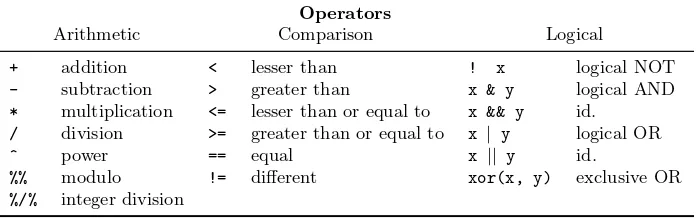
We have seen previously that there are three main types of operators in R10. Here is the list.
Operators
Arithmetic Comparison Logical
+ addition < lesser than ! x logical NOT
- subtraction > greater than x & y logical AND
* multiplication <= lesser than or equal to x && y id.
/ division >= greater than or equal to x | y logical OR
^ power == equal x || y id.
%% modulo != different xor(x, y) exclusive OR
%/% integer division
The arithmetic and comparison operators act on two elements (x + y, a < b). The arithmetic operators act not only on variables of mode numeric or complex, but also on logical variables; in this latter case, the logical values are coerced into numeric. The comparison operators may be applied to any mode: they return one or several logical values.
The logical operators are applied to one (!) or two objects of mode logical, and return one (or several) logical values. The operators “AND” and “OR” exist in two forms: the single one operates on each elements of the objects and returns as many logical values as comparisons done; the double one operates on the first element of the objects.
It is necessary to use the operator “AND” to specify an inequality of the type 0< x <1 which will be coded with: 0 < x & x < 1. The expression 0 < x < 1is valid, but will not return the expected result: since both operators are the same, they are executed successively from left to right. The comparison
0 < x is first done and returns a logical value which is then compared to 1 (TRUE or FALSE < 1): in this situation, the logical value is implicitly coerced into numeric (1or 0 < 1).
10
The following characters are also operators for R:$, @, [,[[, :, ?,<-, <<-, =, ::. A
> x <- 0.5 > 0 < x < 1 [1] FALSE
The comparison operators operate on each element of the two objects being compared (recycling the values of the shortest one if necessary), and thus returns an object of the same size. To compare ‘wholly’ two objects, two functions are available: identicaland all.equal.
> x <- 1:3; y <- 1:3 > x == y
[1] TRUE TRUE TRUE > identical(x, y) [1] TRUE
> all.equal(x, y) [1] TRUE
identical compares the internal representation of the data and returns
TRUE if the objects are strictly identical, and FALSE otherwise. all.equal
compares the “near equality” of two objects, and returns TRUE or display a summary of the differences. The latter function takes the approximation of the computing process into account when comparing numeric values. The comparison of numeric values on a computer is sometimes surprising!
> 0.9 == (1 - 0.1) [1] TRUE
> identical(0.9, 1 - 0.1) [1] TRUE
> all.equal(0.9, 1 - 0.1) [1] TRUE
> 0.9 == (1.1 - 0.2) [1] FALSE
> identical(0.9, 1.1 - 0.2) [1] FALSE
> all.equal(0.9, 1.1 - 0.2) [1] TRUE
> all.equal(0.9, 1.1 - 0.2, tolerance = 1e-16) [1] "Mean relative difference: 1.233581e-16"
3.5.4 Accessing the values of an object: the indexing system
The indexing system is an efficient and flexible way to access selectively the elements of an object; it can be either numeric or logical. To access, for example, the third value of a vector x, we just type x[3] which can be used either to extract or to change this value:
> x[3] [1] 3
> x[3] <- 20 > x
[1] 1 2 20 4 5
The index itself can be a vector of mode numeric:
> i <- c(1, 3) > x[i]
[1] 1 20
If xis a matrix or a data frame, the value of the ith line and jth column is accessed with x[i, j]. To access all values of a given row or column, one has simply to omit the appropriate index (without forgetting the comma!):
> x <- matrix(1:6, 2, 3) > x
[,1] [,2] [,3]
[1,] 1 3 5
[2,] 2 4 6
> x[, 3] <- 21:22 > x
[,1] [,2] [,3]
[1,] 1 3 21
[2,] 2 4 22
> x[, 3] [1] 21 22
You have certainly noticed that the last result is a vector and not a matrix. The default behaviour of R is to return an object of the lowest dimension possible. This can be altered with the option dropwhich default isTRUE:
> x[, 3, drop = FALSE] [,1]
[1,] 21
[2,] 22
This indexing system is easily generalized to arrays, with as many indices as the number of dimensions of the array (for example, a three dimensional array: x[i, j, k],x[, , 3],x[, , 3, drop = FALSE], and so on). It may be useful to keep in mind that indexing is made with square brackets, while parentheses are used for the arguments of a function:
> x(1)
Indexing can also be used to suppress one or several rows or columns using negative values. For example,x[-1, ]will suppress the first row, while
x[-c(1, 15), ]will do the same for the 1st and 15th rows. Using the matrix defined above:
> x[, -1] [,1] [,2]
[1,] 3 21
[2,] 4 22
> x[, -(1:2)] [1] 21 22
> x[, -(1:2), drop = FALSE] [,1]
[1,] 21
[2,] 22
For vectors, matrices and arrays, it is possible to access the values of an element with a comparison expression as the index:
> x <- 1:10
> x[x >= 5] <- 20 > x
[1] 1 2 3 4 20 20 20 20 20 20 > x[x == 1] <- 25
> x
[1] 25 2 3 4 20 20 20 20 20 20
A practical use of the logical indexing is, for instance, the possibility to select the even elements of an integer variable:
> x <- rpois(40, lambda=5) > x
[1] 5 9 4 7 7 6 4 5 11 3 5 7 1 5 3 9 2 2 5 2
[21] 4 6 6 5 4 5 3 4 3 3 3 7 7 3 8 1 4 2 1 4
> x[x %% 2 == 0]
[1] 4 6 4 2 2 2 4 6 6 4 4 8 4 2 4
Thus, this indexing system uses the logical values returned, in the above examples, by comparison operators. These logical values can be computed beforehand, they then will be recycled if necessary:
> x <- 1:40
> s <- c(FALSE, TRUE) > x[s]
Logical indexing can also be used with data frames, but with caution since different columns of the data drame may be of different modes.
For lists, accessing the different elements (which can be any kind of object) is done either with single or with double square brackets: the difference is that with single brackets a list is returned, whereas double bracketsextractthe object from the list. The result can then be itself indexed as previously seen for vectors, matrices, etc. For instance, if the third object of a list is a vector, its
ith value can be accessed using my.list[[3]][i], if it is a three dimensional array using my.list[[3]][i, j, k], and so on. Another difference is that
my.list[1:2] will return a list with the first and second elements of the original list, whereasmy.list[[1:2]]will no not give the expected result.
3.5.5 Accessing the values of an object with names
The namesare labels of the elements of an object, and thus of mode charac-ter. They are generally optional attributes. There are several kinds of names (names,colnames,rownames, dimnames).
The names of a vector are stored in a vector of the same length of the object, and can be accessed with the function names.
> x <- 1:3 > names(x) NULL
> names(x) <- c("a", "b", "c") > x
a b c 1 2 3 > names(x) [1] "a" "b" "c" > names(x) <- NULL > x
[1] 1 2 3
For matrices and data frames, colnames and rownames are labels of the columns and rows, respectively. They can be accessed either with their re-spective functions, or withdimnameswhich returns a list with both vectors.
> X <- matrix(1:4, 2)
> rownames(X) <- c("a", "b") > colnames(X) <- c("c", "d") > X
c d a 1 3 b 2 4
> dimnames(X) [[1]]
[[2]]
[1] "c" "d"
For arrays, the names of the dimensions can be accessed with dimnames:
> A <- array(1:8, dim = c(2, 2, 2)) > A
, , 1
[,1] [,2]
[1,] 1 3
[2,] 2 4
, , 2
[,1] [,2]
[1,] 5 7
[2,] 6 8
> dimnames(A) <- list(c("a", "b"), c("c", "d"), c("e", "f")) > A
, , e
c d a 1 3 b 2 4
, , f
c d a 5 7 b 6 8
If the elements of an object have names, they can be extracted by using them as indices. Actually, this should be termed ‘subsetting’ rather than ‘extraction’ since the attributes of the original object are kept. For instance, if a data frameDF contains the variables x,y, and z, the command DF["x"]
will return a data frame with just x; DF[c("x", "y")] will return a data frame with both variables. This works with lists as well if the elements in the list have names.
As the reader surely realizes, the index used here is a vector of mode character. Like the numeric or logical vectors seen above, this vector can be defined beforehand and then used for the extraction.
To extract a vector or a factor from a data frame, on can use the operator
3.5.6 The data editor
It is possible to use a graphical spreadsheet-like editor to edit a “data” object. For example, ifXis a matrix, the commanddata.entry(X)will open a graphic editor and one will be able to modify some values by clicking on the appropriate cells, or to add new columns or rows.
The function data.entry modifies directly the object given as argument without needing to assign its result. On the other hand, the function de
returns a list with the objects given as arguments and possibly modified. This result is displayed on the screen by default, but, as for most functions, can be assigned to an object.
The details of using the data editor depend on the operating system.
3.5.7 Arithmetics and simple functions
There are numerous functions in R to manipulate data. We have already seen the simplest one, cwhich concatenates the objects listed in parentheses. For example:
> c(1:5, seq(10, 11, 0.2))
[1] 1.0 2.0 3.0 4.0 5.0 10.0 10.2 10.4 10.6 10.8 11.0
Vectors can be manipulated with classical arithmetic expressions:
> x <- 1:4
> y <- rep(1, 4) > z <- x + y > z
[1] 2 3 4 5
Vectors of different lengths can be added; in this case, the shortest vector is recycled. Examples:
> x <- 1:4 > y <- 1:2 > z <- x + y > z
[1] 2 4 4 6 > x <- 1:3 > y <- 1:2 > z <- x + y Warning message: longer object length
is not a multiple of shorter object length in: x + y > z
Note that R returned a warning message and not an error message, thus the operation has been performed. If we want to add (or multiply) the same value to all the elements of a vector:
> x <- 1:4 > a <- 10 > z <- a * x > z
[1] 10 20 30 40
The functions available in R for manipulating data are too many to be listed here. One can find all the basic mathematical functions (log, exp,
log10,log2,sin,cos, tan,asin,acos, atan, abs,sqrt, . . . ), special func-tions (gamma,digamma,beta,besselI, . . . ), as well as diverse functions useful in statistics. Some of these functions are listed in the following table.
sum(x) sum of the elements of x
prod(x) product of the elements of x
max(x) maximum of the elements of x
min(x) minimum of the elements of x
which.max(x) returns the index of the greatest element ofx
which.min(x) returns the index of the smallest element of x
range(x) id. thanc(min(x), max(x))
length(x) number of elements inx
mean(x) mean of the elements of x
median(x) median of the elements of x
var(x)orcov(x) variance of the elements of x (calculated on n−1); if x is
a matrix or a data frame, the variance-covariance matrix is calculated
cor(x) correlation matrix of xif it is a matrix or a data frame (1 if x
is a vector)
var(x, y)orcov(x, y) covariance betweenxandy, or between the columns of xand
those of yif they are matrices or data frames
cor(x, y) linear correlation betweenxandy, or correlation matrix if they
are matrices or data frames
These functions return a single value (thus a vector of length one), except
rangewhich returns a vector of length two, andvar,cov, andcorwhich may return a matrix. The following functions return more complex results.
round(x, n) rounds the elements of xtondecimals
rev(x) reverses the elements of x
sort(x) sorts the elements ofxin increasing order; to sort in decreasing order:
rev(sort(x))
log(x, base) computes the logarithm of xwith basebase
scale(x) if x is a matrix, centers and reduces the data; to center only use
the option center=FALSE, to reduce only scale=FALSE (by default
center=TRUE, scale=TRUE)
pmin(x,y,...) a vector whichith element is the minimum ofx[i],y[i], . . .
pmax(x,y,...) id. for the maximum
cumsum(x) a vector whichith element is the sum fromx[1]tox[i]
cumprod(x) id. for the product
cummin(x) id. for the minimum
cummax(x) id. for the maximum
match(x, y) returns a vector of the same length than x with the elements of x
which are iny(NAotherwise)
which(x == a) returns a vector of the indices of x if the comparison operation is
true (TRUE), in this example the values ofifor whichx[i] == a(the
argument of this function must be a variable of mode logical)
choose(n, k) computes the combinations ofkevents amongnrepetitions =n!/[(n−
k)!k!]
na.omit(x) suppresses the observations with missing data (NA) (suppresses the
corresponding line ifxis a matrix or a data frame)
na.fail(x) returns an error message if xcontains at least oneNA
unique(x) if xis a vector or a data frame, returns a similar object but with the
duplicate elements suppressed
table(x) returns a table with the numbers of the differents values ofx(typically
for integers or factors)
table(x, y) contingency table of xandy
subset(x, ...) returns a selection of xwith respect to criteria (..., typically
com-parisons: x$V1 < 10); if x is a data frame, the option select gives
the variables to be kept (or dropped using a minus sign)
sample(x, size) resample randomly and without replacement size elements in the
vectorx, the optionreplace = TRUEallows to resample with
replace-ment
3.5.8 Matrix computation
R has facilities for matrix computation and manipulation. The functions
rbind and cbind bind matrices with respect to the lines or the columns, respectively:
> m1 <- matrix(1, nr = 2, nc = 2) > m2 <- matrix(2, nr = 2, nc = 2) > rbind(m1, m2)
[,1] [,2]
[1,] 1 1
[2,] 1 1
[3,] 2 2
[4,] 2 2
> cbind(m1, m2)
[1,] 1 1 2 2
[2,] 1 1 2 2
The operator for the product of two matrices is ‘%*%’. For example, con-sidering the two matricesm1 andm2 above:
> rbind(m1, m2) %*% cbind(m1, m2) [,1] [,2] [,3] [,4]
[1,] 2 2 4 4
[2,] 2 2 4 4
[3,] 4 4 8 8
[4,] 4 4 8 8
> cbind(m1, m2) %*% rbind(m1, m2) [,1] [,2]
[1,] 10 10
[2,] 10 10
The transposition of a matrix is done with the function t; this function works also with a data frame.
The function diag can be used to extract or modify the diagonal of a matrix, or to build a diagonal matrix.
> diag(m1) [1] 1 1
> diag(rbind(m1, m2) %*% cbind(m1, m2)) [1] 2 2 8 8
> diag(m1) <- 10 > m1
[,1] [,2]
[1,] 10 1
[2,] 1 10
> diag(3)
[,1] [,2] [,3]
[1,] 1 0 0
[2,] 0 1 0
[3,] 0 0 1
> v <- c(10, 20, 30) > diag(v)
[,1] [,2] [,3]
[1,] 10 0 0
[2,] 0 20 0
[3,] 0 0 30
> diag(2.1, nr = 3, nc = 5) [,1] [,2] [,3] [,4] [,5]
[1,] 2.1 0.0 0.0 0 0
[2,] 0.0 2.1 0.0 0 0
4
Graphics with R
R offers a remarkable variety of graphics. To get an idea, one can type
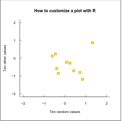
demo(graphics) or demo(persp). It is not possible to detail here the pos-sibilities of R in terms of graphics, particularly since each graphical function has a large number of options making the production of graphics very flexible. The way graphical functions work deviates substantially from the scheme sketched at the beginning of this document. Particularly, the result of a graph-ical function cannot be assigned to an object11but is sent to agraphical device.
A graphical device is a graphical window or a file.
There are two kinds of graphical functions: the high-level plotting func-tions which create a new graph, and the low-level plotting functions which add elements to an existing graph. The graphs are produced with respect to graphical parameters which are defined by default and can be modified with the functionpar.
We will see in a first time how to manage graphics and graphical devices; we will then somehow detail the graphical functions and parameters. We will see a practical example of the use of these functionalities in producing graphs. Finally, we will see the packagesgrid andlatticewhose functioning is different from the one summarized above.
4.1 Managing graphics
4.1.1 Opening several graphical devices
When a graphical function is executed, if no graphical device is open, R opens a graphical window and displays the graph. A graphical device may be open with an appropriate function. The list of available graphical devices depends on the operating system. The graphical windows are called X11 under Unix/Linux and windows under Windows. In all cases, one can open a graphical window with the commandx11()which also works under Windows because of an alias towards the command windows(). A graphical device which is a file will be open with a function depending on the format: postscript(),pdf(),png(), . . . The list of available graphical devices can be found with?device.
The last open device becomes the active graphical device on which all subsequent graphs are displayed. The function dev.list() displays the list of open devices:
> x11(); x11(); pdf() > dev.list()
11
There are a few remarkable exceptions: hist() and barplot() produce also numeric
X11 X11 pdf
2 3 4
The figures displayed are the device numbers which must be used to change the active device. To know what is the active device:
> dev.cur() pdf
4
and to change the active device:
> dev.set(3) X11
3
The function dev.off() closes a device: by default the active device is closed, otherwise this is the one which number is given as argument to the function. R then displays the number of the new active device:
> dev.off(2) X11
3
> dev.off() pdf
4
Two specific features of the Windows version of R are worth mentioning: a Windows Metafile device can be open with the functionwin.metafile, and a menu “History” displayed when the graphical window is selected allowing recording of all graphs drawn during a session (by default, the recording system is off, the user switches it on by clicking on “Recording” in this menu).
4.1.2 Partitioning a graphic
The functionsplit.screenpartitions the active graphical device. For exam-ple:
> split.screen(c(1, 2))
divides the device into two parts which can be selected with screen(1) or
screen(2); erase.screen() deletes the last drawn graph. A part of the device can itself be divided withsplit.screen()leading to the possibility to make complex arrangements.
These functions are incompatible with others (such as layoutor coplot) and must not be used with multiple graphical devices. Their use should be limited, for instance, to graphical exploration of data.
> layout(matrix(1:4, 2, 2))
It is of course possible to create this matrix previously allowing to better visualize how the device is divided:
> mat <- matrix(1:4, 2, 2) > mat
[,1] [,2]
[1,] 1 3
[2,] 2 4
> layout(mat)
To actually visualize the partition created, one can use the functionlayout.show
with the number of sub-windows as argument (here 4). In this example, we will have:
> layout.show(4)
1
2 3
4
The following examples show some of the possibilities offered bylayout().
> layout(matrix(1:6, 3, 2)) > layout.show(6)
1
2
3 4
5
6
> layout(matrix(1:6, 2, 3)) > layout.show(6)
1
2 3
4 5
6
> m <- matrix(c(1:3, 3), 2, 2) > layout(m)
> layout.show(3)
1
2 3
in the matrix may also be given in any order, for example, matrix(c(2, 1, 4, 3), 2, 2).
By default,layout()partitions the device with regular heights and widths: this can be modified with the optionswidthsandheights. These dimensions are given relatively12. Examples:
> m <- matrix(1:4, 2, 2) > layout(m, widths=c(1, 3),
heights=c(3, 1)) > layout.show(4)
1
2 3
4
> m <- matrix(c(1,1,2,1),2,2) > layout(m, widths=c(2, 1),
heights=c(1, 2)) > layout.show(2)
1 2
Finally, the numbers in the matrix can include zeros giving the possibility to make complex (or even esoterical) partitions.
> m <- matrix(0:3, 2, 2) > layout(m, c(1, 3), c(1, 3))
> layout.show(3) 1
2
3
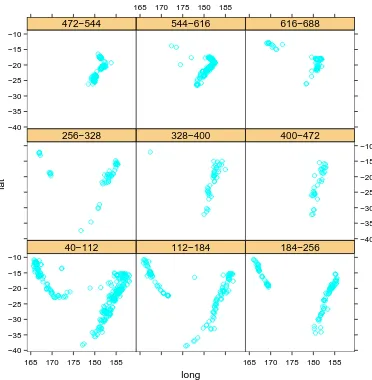
> m <- matrix(scan(), 5, 5) 1: 0 0 3 3 3 1 1 3 3 3 11: 0 0 3 3 3 0 2 2 0 5 21: 4 2 2 0 5
26:
Read 25 items > layout(m) > layout.show(5)
1
2
3
4
5
12
4.2 Graphical functions
Here is an overview of the high-level graphical functions in R.
plot(x) plot of the values of x(on they-axis) ordered on thex-axis
plot(x, y) bivariate plot of x(on thex-axis) andy(on they-axis)
sunflowerplot(x, y)
id. but the points with similar coordinates are drawn as a flower which petal number represents the number of points
pie(x) circular pie-chart
boxplot(x) “box-and-whiskers” plot
stripchart(x) plot of the values ofxon a line (an alternative toboxplot()for
small sample sizes)
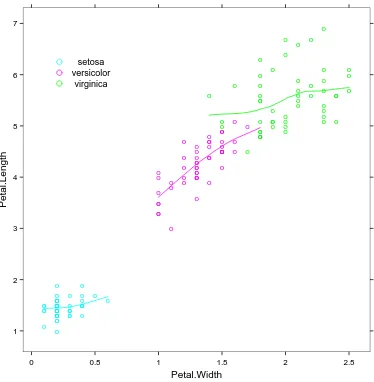
coplot(x~y | z) bivariate plot of xandyfor each value (or interval of values) of
z interaction.plot (f1, f2, y)
iff1andf2are factors, plots the means ofy(on they-axis) with
respect to the values of f1(on thex-axis) and of f2 (different
curves); the option funallows to choose the summary statistic
of y(by defaultfun=mean)
matplot(x,y) bivariate plot of the first column of xvs.the first one of y, the
second one of xvs.the second one ofy, etc.
dotchart(x) if x is a data frame, plots a Cleveland dot plot (stacked plots
line-by-line and column-by-column)
fourfoldplot(x) visualizes, with quarters of circles, the association between two
dichotomous variables for different populations (x must be an
array with dim=c(2, 2, k), or a matrix with dim=c(2, 2) if
k= 1)
assocplot(x) Cohen–Friendly graph showing the deviations from
indepen-dence of rows and columns in a two dimensional contingency table
mosaicplot(x) ‘mosaic’ graph of the residuals from a log-linear regression of a
contingency table
pairs(x) ifxis a matrix or a data frame, draws all possible bivariate plots
between the columns of x
plot.ts(x) if xis an object of class"ts", plot of xwith respect to time,x
may be multivariate but the series must have the same frequency and dates
ts.plot(x) id. but if xis multivariate the series may have different dates
and must have the same frequency
hist(x) histogram of the frequencies of x
barplot(x) histogram of the values of x
qqnorm(x) quantiles ofxwith respect to the values expected under a normal
law
qqplot(x, y) quantiles of ywith respect to the quantiles of x
contour(x, y, z) contour plot (data are interpolated to draw the curves), x
and y must be vectors and z must be a matrix so that
dim(z)=c(length(x), length(y)) (xandymay be omitted)
filled.contour (x, y, z)
id. but the areas between the contours are coloured, and a legend of the colours is drawn as well
image(x, y, z) id. but the actual data are represented with colours
persp(x, y, z) id. but in perspective
stars(x) if xis a matrix or a data frame, draws a graph with segments
or a star where each row of xis represented by a star and the