Introduction to the R Project for Statistical Computing
for use at ITC
D G Rossiter University of Twente Faculty of Geo-information Science & Earth Observation (ITC) Enschede (NL)
http:// www.itc.nl/ personal/ rossiter
August 14, 2012
●
Actual vs. modelled straw yields
●
Grain yield, lbs per plot
Frequency histogram, Meuse lead concentration
Counts shown above bar, actual values shown with rug plot lead concentration, mg kg−1
Frequency
660000 670000 680000 690000 700000
315000
GLS 2nd−order trend surface, subsoil clay %
E
Contents
0 If you are impatient . . . 1
1 What is R? 1 2 Why R for ITC? 3 2.1 Advantages . . . 3
2.2 Disadvantages . . . 4
2.3 Alternatives . . . 5
2.3.1 S-PLUS . . . 5
2.3.2 Statistical packages . . . 5
2.3.3 Special-purpose statistical programs . . . 5
2.3.4 Spreadsheets . . . 6
2.3.5 Applied mathematics programs . . . 6
3 Using R 7 3.1 R console GUI . . . 7
3.1.1 On your own Windows computer . . . 7
3.1.2 On the ITC network . . . 7
3.1.3 Running the R console GUI . . . 8
3.1.4 Setting up a workspace in Windows . . . 8
3.1.5 Saving your analysis steps . . . 9
3.1.6 Saving your graphs . . . 9
3.2 Working with the R command line . . . 10
3.2.1 The command prompt . . . 10
3.2.2 On-line help in R . . . 11
3.3 TheRStudiodevelopment environment . . . 13
3.4 TheTinn-Rcode editor . . . 14
3.5 Writing and running scripts . . . 14
3.6 TheRcmdrGUI . . . 16
3.7 Loading optional packages. . . 17
3.8 Sample datasets . . . 18
4 The S language 19 4.1 Command-line calculator and mathematical operators . . . . 19
4.2 Creating new objects: the assignment operator . . . 20
4.3 Methods and their arguments . . . 21
4.4 Vectorized operations and re-cycling . . . 22
4.5 Vector and list data structures . . . 24
4.6 Arrays and matrices . . . 25
4.7 Data frames . . . 30
4.8 Factors . . . 34
4.9 Selecting subsets . . . 36
4.9.1 Simultaneous operations on subsets . . . 39
4.10 Rearranging data . . . 40
4.11 Random numbers and simulation . . . 41
4.12 Character strings. . . 43
4.13 Objects and classes . . . 44
4.13.1 The S3 and S4 class systems . . . 45
4.14 Descriptive statistics . . . 48
4.15 Classification tables . . . 50
4.16 Sets . . . 51
4.17 Statistical models in S. . . 52
4.17.1 Models with categorical predictors . . . 55
4.17.2 Analysis of Variance (ANOVA) . . . 57
4.18 Model output . . . 57
4.18.1 Model diagnostics . . . 59
4.18.2 Model-based prediction . . . 61
4.19 Advanced statistical modelling . . . 62
4.20 Missing values . . . 63
4.21 Control structures and looping . . . 64
4.22 User-defined functions . . . 65
4.23 Computing on the language . . . 67
5 R graphics 69 5.1 Base graphics . . . 69
5.1.1 Mathematical notation in base graphics . . . 73
5.1.2 Returning results from graphics methods . . . 75
5.1.3 Types of base graphics plots . . . 75
5.1.4 Interacting with base graphics plots. . . 77
5.2 Trellis graphics . . . 77
5.2.1 Univariate plots . . . 77
5.2.2 Bivariate plots . . . 78
5.2.3 Triivariate plots . . . 79
5.2.4 Panel functions. . . 81
5.2.5 Types of Trellis graphics plots . . . 82
5.2.6 Adjusting Trellis graphics parameters . . . 82
5.3 Multiple graphics windows. . . 84
5.3.1 Switching between windows. . . 85
5.4 Multiple graphs in the same window . . . 85
5.4.1 Base graphics . . . 85
5.4.2 Trellis graphics. . . 86
5.5 Colours. . . 86
6 Preparing your own data for R 91 6.1 Preparing data directly in R . . . 91
6.2 A GUI data editor . . . 92
6.3 Importing data from a CSV file . . . 93
6.4 Importing images . . . 96
8 Reproducible data analysis 101
8.1 The NoWeb document . . . 101
8.2 The LATEX document . . . 102
8.3 The PDF document . . . 103
8.4 Graphics in Sweave . . . 104
9 Learning R 105 9.1 Task views. . . 105
9.2 R tutorials and introductions . . . 105
9.3 Textbooks using R . . . 106
9.4 Technical notes using R . . . 107
9.5 Web Pages to learn R . . . 107
9.6 Keeping up with developments in R . . . 108
10 Frequently-asked questions 110 10.1 Help! I got an error, what did I do wrong? . . . 110
10.2 Why didn’t my command(s) do what I expected? . . . 112
10.3 How do I find the method to do what I want? . . . 113
10.4 Memory problems . . . 115
10.5 What version of R am I running? . . . 116
10.6 What statistical procedure should I use? . . . 117
A Obtaining your own copy of R 119 A.1 Installing new packages . . . 121
A.2 Customizing your installation. . . 121
A.3 R in different human languages. . . 122
B An example script 123 C An example function 126 References 128 Index of R concepts 133 List of Figures 1 The RStudio screen . . . 13
2 The Tinn-R screen . . . 14
3 The R Commander screen . . . 16
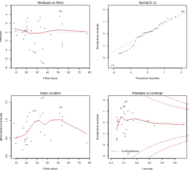
4 Regression diagnostic plots . . . 60
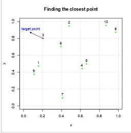
5 Finding the closest point . . . 66
6 Default scatterplot. . . 70
7 Plotting symbols . . . 71
8 Custom scatterplot . . . 73
9 Scatterplot with math symbols, legend and model lines. . . . 74
10 Some interesting base graphics plots . . . 76
11 Trellis density plots . . . 78
12 Trellis scatter plots . . . 79
13 Trellis trivariate plots . . . 80
15 Available colours. . . 87
16 Example of a colour ramp . . . 89
17 R graphical data editor . . . 93
18 Example PDF produced by Sweave and LATEX . . . . 103
19 Results of an RSeek search. . . 108
20 Results of an R site search . . . 109
21 Visualising the variability of small random samples . . . 125
List of Tables 1 Methods for adding to an existing base graphics plot . . . 71
2 Base graphics plot types . . . 75
3 Trellis graphics plot types . . . 83
0 If you are impatient . . .
1. Install R and RStudio on your MS-Windows, Mac OS/X or Linux sys-tem (§A);
2. Run RStudio; this will automatically start R within it;
3. Follow one of the tutorials (§9.2) such as my “Using the R Environ-ment for Statistical Computing: An example with the Mercer & Hall wheat yield dataset”1[48];
4. Experiment!
5. Use this document as a reference.
1 What is R?
R is an open-source environment for statistical computing and visualisa-tion. It is based on the S language developed at Bell Laboratories in the 1980’s [20], and is the product of an active movement among statisti-cians for a powerful, programmable, portable, and open computing en-vironment, applicable to the most complex and sophsticated problems, as well as “routine” analysis, without any restrictions on access or use. Here is a description from the R Project home page:2
“R is anintegrated suite of software facilitiesfor data manip-ulation, calculation and graphical display. It includes:
• an effectivedata handling and storagefacility,
• a suite of operators for calculations on arrays, in partic-ularmatrices,
• a large, coherent, integrated collection ofintermediate tools for data analysis,
• graphical facilitiesfor data analysis and display either on-screen or on hardcopy, and
• a well-developed, simple and effective programming lan-guagewhich includes conditionals, loops, user-defined re-cursive functions and input and output facilities.”
The last point has resulted in another major feature:
• Practising statisticianshave implemented hundreds of
spe-1http://www.itc.nl/personal/rossiter/pubs/list.html#pubs_m_R, item 2
cialised statistical produres for a wide variety of appli-cations as contributed packages, which are also freely-available and which integrate directly into R.
A few examples especially relevant to ITC’s mission are:
• the gstat, geoR and spatial packages for geostatistical analysis, contributed by Pebesma [33], Ribeiro, Jr. & Diggle [39] and Ripley [40], respectively;
• thespatstatpackage for spatial point-pattern analysis and simula-tion;
• theveganpackage of ordination methods for ecology;
• thecircularpackage for directional statistics;
• thesppackage for a programming interface to spatial data;
• thergdalpackage for GDAL-standard data access to geographic data sources;
There are also packages for the most modern statistical techniques such as:
• sophisticated modelling methods, including generalized linear mod-els, principal components, factor analysis, bootstrapping, and robust regression; these are listed in §4.19;
• wavelets (wavelet);
• neural networks (nnet);
• non-linear mixed-effects models (nlme);
• recursive partitioning (rpart);
• splines (splines);
2 Why R for ITC?
“ITC” is an abbreviation for University of Twente, Faculty of Geo-information Science& Earth Observation. It is a faculty of the University of Twente lo-cated in Enschede, the Netherlands, with a thematic focus on geo-information science and earth observation in support of development. Thus the two pillars on which ITC stands aredevelopment-related andgeo-information. R supports both of these.
2.1 Advantages
R has several majoradvantagesfor a typical ITC student or collaborator:
1. It iscompletely free and will always be so, since it is issued under the GNU Public License;3
2. It isfreely-available over the internet, via a large network ofmirror
servers; see Appendix Afor how to obtain R;
3. It runs on many operating systems: Unix© and derivatives includ-ing Darwin, Mac OS X, Linux, FreeBSD, and Solaris; most flavours of Microsoft Windows; Apple Macintosh OS; and even some mainframe OS.
4. It is the product ofinternational collaborationbetweentop compu-tational statisticiansand computer language designers;
5. It allowsstatistical analysisandvisualisationofunlimited sophisti-cation; you are not restricted to a small set of procedures or options, and because of the contributed packages, you are not limited to one method of accomplishing a given computation or graphical presen-tation;
6. It can work onobjects of unlimited size and complexitywith a con-sistent, logicalexpression language;
7. It is supported by comprehensivetechnical documentationand user-contributed tutorials (§9). There are also several good textbooks on statistical methods that use R (or S) for illustration.
8. Every computational step isrecorded, and this history can be saved for later use or documentation.
9. It stimulates critical thinking about problem-solving rather than a “push the button” mentality.
10. It is fully programmable, with its own sophisticated computer lan-guage (§4). Repetitive procedures can easily be automated by
written scripts (§3.5). It is easy to write your own functions (§B), and not too difficult to write wholepackagesif you invent some new analysis;
11. Allsource codeis published, so you can see the exact algorithms be-ing used; also, expert statisticians can make sure the code is correct;
12. It can exchange datain MS-Excel, text, fixed and delineated formats (e.g. CSV), so that existing datasets are easily imported (§6), and re-sults computed in R are easily exported (§7).
13. Most programs written for the commercial S-PLUS program will run unchanged, or with minor changes, in R (§2.3.1).
2.2 Disadvantages
R has itsdisadvantages(although “every disadvantage has its advantage”):
1. The default Windows and Mac OS X graphical user interface (GUI) (§3.1) is limited to simple system interaction and does not include statistical procedures. The user musttype commandsto enter data, do analyses, and plot graphs. This has the advantage that the user has complete control over the system. The Rcmdr add-on package (§3.6) provides a reasonable GUI for common tasks, and there are various development environments for R, such as RStudio (§3.3).
2. The user must decide on theanalysis sequenceand execute it step-by-step. However, it is easy to create scripts with all the steps in an analysis, and run the script from the command line or menus (§3.5); scripts can be preared in code editors built into GUI versions of R or separate front-ends such as Tinn-R (§3.5) or RStudio (§3.3). A major advantage of this approach is that intermediate results can be reviewed, and scripts can be edited and run as batch processes.
3. The user must learn a new way of thinking about data, as data frames(§4.7) andobjectseach with itsclass, which in turn supports a set of methods(§4.13). This has the advantage common to object-oriented languages that you can only operate on an object according to methods that make sense4 and methods can adapt to the type of object.5
4. The user must learn the S language (§4), both for commands and the notation used to specify statistical models(§4.17). The S statis-tical modelling language is a lingua franca among statisticians, and provides a compact way to express models.
4For example, thet(transpose) method only can be applied to matrices
5For example, thesummaryandplotmethods give different results depending on the
2.3 Alternatives
There are many ways to do computational statistics; this section discusses them in relation to R. None of these programs are open-source, meaning that you must trust the company to do the computations correctly.
2.3.1 S-PLUS
S-PLUS is a commercial program distributed by the Insightful corporation,6
and is a popular choice for large-scale commerical statistical computing. Like R, it is a dialect of the original S language developed at Bell Laborato-ries.7 S-PLUS has a full graphical user interface (GUI); it may be also used
like R, by typing commands at the command line interface or by running scripts. It has a rich interactive graphics environment called Trellis, which has been emulated with thelatticepackage in R (§5.2). S-PLUS is licensed by local distributors in each country at prices ranging from moderate to high, depending factors such as type of licensee and application, and how many computers it will run on. The important point for ITC R users is that their expertise will be immediately applicable if they later use S-PLUS in a commercial setting.
2.3.2 Statistical packages
There are many statistical packages, including MINITAB, SPSS, Statistica, Systat, GenStat, and BMDP,8which are attractive if you are already familiar
with them or if you are required to use them at your workplace. Although these are programmable to varying degrees, it is not intended that special-ists develop completely new algorithms. These must be purchased from local distributors in each country, and the purchaser must agree to the li-cense terms. These often have common analyses built-in as menu choices; these can be convenient but it is tempting to use them without fully un-derstanding what choices they are making for you.
SAS is a commercial competitor to S-PLUS, and is used widely in industry. It is fully programmable with a language descended from PL/I (used on IBM mainframe computers).
2.3.3 Special-purpose statistical programs
Some programs adress specific statistical issues, e.g. geostatistical analysis and interpolation (SURFER, gslib, GEO-EAS), ecological analysis (FRAG-STATS), and ordination (CONOCO). The algorithms in these programs have
6http://www.insightful.com/
7There are differences in the language definitions of S, R, and S-PLUS that are important
to programmers, but rarely to end-users. There are also differences in how some algorithms are implemented, so the numerical results of an identical method may be somewhat different.
or can be programmed as an R package; examples are thegstatprogram for geostatistical analysis9 [35], which is now available within R [33], and
theveganpackage for ecological statistics.
2.3.4 Spreadsheets
Microsoft Excel is useful for data manipulation. It can also calculate some statistics (means, variances, . . . ) directly in the spreadsheet. This is also an add-on module (menu item Tools|Data Analysis. . . ) for some common statistical procedures including random number generation. Be aware that Excel was not designed by statisticians. There are also some commer-cial add-on packages for Excel that provide more sophisticated statistical analyses. Excel’s default graphics are easy to produce, and they may be customized via dialog boxes, but their design has been widely criticized. Least-squares fits on scatterplots give no regression diagnostics, so this is not a serious linear modelling tool.
OpenOffice10 includes an open-source and free spreadsheet (Open Office Calc) which can replace Excel.
2.3.5 Applied mathematics programs
MATLAB is a widely-used applied mathematics program, especially suited to matrix maniupulation (as is R, see §4.6), which lends itself naturally to programming statistical algorithms. Add-on packages are available for many kinds of statistical computation. Statistical methods are also pro-grammable in Mathematica.
9http://www.gstat.org/
3 Using R
There are several ways to work with R:
• with theR console GUI(§3.1);
• with theRStudioIDE (§3.3);
• with theTinn-R editorand the R console (§3.4);
• from one of the other IDE such as JGR;
• from a command line R interface (CLI) (§3.2);
• from the ESS (Emacs Speaks Statistics) module of the Emacs editor.
Of these, RStudio is for most ITC users the best choice; it contains an R command line interface but with a code editor, help text, a workspace browser, and graphic output.
3.1 R console GUI
The default interface for both Windows and Mac OS/X is a simple GUI. We refer to these as “R console GUI” because they provide an easy-to-use interface to the R command line, a simple script editor, graphics output, and on-line help; they do not contain any menus for data manipulation or statistical procedures.
R for Linux has no GUI; however, several independent Linux programs11
provide a GUI development environment; an example is RStudio (§3.3).
3.1.1 On your own Windows computer
You can download and install R for Windows as instructed in §A, as for a typical Windows program; this will create a Start menu item and a desktop shortcut.
3.1.2 On the ITC network
R has been installed on the ITC corporate network at:
\\Itcnt03\Apps\R\bin\RGui.exe
For most ITC accounts driveP:has been mapped to\\Itcnt03\Apps, so R can be accessed using this drive letter instead of the network address:
P:\R\bin\RGui.exe
You can copy this to your local desktop as a shortcut.
Documentation has been installed at:
P:\R\doc
3.1.3 Running the R console GUI
R GUI for Windows is started like any Windows program: from the Start menu, from a desktop shortcut, or from the application’s icon in Explorer.
By default, R starts in the directory where it was installed, which is not where you should store your projects. If you are using the copy of R on the ITC network, you do not have write permission to this directory, so you won’t be able to save any data or session information there. So, you will probably want to change your workspace, as explained in §3.1.4. You can also create a desktop shortcut or Start menu item for R, also as explained in §3.1.4.
To stop an R session, type q() at the command prompt12, or select the
File | Exitmenu item in the Windows GUI.
3.1.4 Setting up a workspace in Windows
An important concept in R is the workspace, which contains the local data and procedures for a given statistics project. Under Windows this is usually determined by the folder from which R is started.
Under Windows, the easiest way to set up a statistics project is:
1. Create ashortcuttoRGui.exeon your desktop;
2. Modify its properties so that its in your working directory rather than the default (e.g.P:\R\bin).
Now when you double-click on the shortcut, it will start R in the directory of your choice. So, you can set up a different shortcut for each of your projects.
Another way to set up a new statistics project in R is:
1. Start R as just described:double-click the iconfor programRGui.exe
in the Explorer;
2. Select theFile | Change Directory ... menu item in R;
3. Select the directory where you want to work;
4. Exit R by selecting theFile | Exit menu item in R, or typing the
q() command; R will ask “Save workspace image?”; Answery(Yes). This will create two files in your working directory: .Rhistory and
.RData.
The next time you want to work on the same project:
1. Open Explorer and navigate to the working directory
2. Double-click on the iconfor file.RData
R should open in that directory, with your previous workspace already loaded. (If R does not open, instead Explorer will ask you what programs should open files of type.RData; navigate to the program RGui.exe and select it.)
If you don’t see the file.RDatain your Explorer, this is because Windows considers any file name that begins with “.” to be a ‘hidden’ file. You need Revealing
hid-den files in Windows
to select the Tools | Folder options in Explorer, then the View tab, and click the radio button for Show hidden files and folders. You must alsoun-check the boxforHide file extensions for known file
types.
3.1.5 Saving your analysis steps
TheFile | Save to file ... menu command will save the entire
con-sole contents, i.e. both your commands and R’s response, to a text file, which you can later review and edit with any text editor. This is useful for cutting-and-pasting into your reports or thesis, and also for writing scripts to repeat procedures.
3.1.6 Saving your graphs
In the Windows version of R, you can save any graphical output for in-sertion into documents or printing. If necessary, bring the graphics win-dow to the front (e.g. click on its title bar), select menu commandFile |
Save as ..., and then one of the formats. Most useful for insertion into
MS-Word documents is Metafile; most useful for LATEX is Postscript; most useful forPDFLaTeXand stand-alone printing is PDF. You can later review your saved graphics with programs such as Windows Picture Editor. If you want to add other graphical elements, you may want to save as a PNG or JPEG; however in most cases it is cleaner to add annotations within R itself.
You can also write your graphics commands directly to a graphics file in many formats, e.g. PDF or JPEG. You do this by opening a graphics device, writing the commands, and then closing the device. You can get a list of graphics devices (formats) available on your system with?Devices(note the upper-caseD).
For example, to write a PDF file, we open a PDF graphics device with the
pdffunction, write to it, and then close it with thedev.offfunction:
pdf("figure1.pdf", h=6, w=6)
hist(rnorm(100), main="100 random values from N[0,1])") dev.off()
Note the use of the optionalheight=andwidth=arguments (here abbre-viatedh= and w=) to specifiy the size of the PDF file (in US inches); this affects the font sizes. The defaults are both 7 inches (17.18 cm).
3.2 Working with the R command line
These instructions apply to the simple R GUI and the R command line interface window within RStudio. One of the windows in these interfaces is the command line, also called the R console.
It is possible to work directly with the command line and no GUI:
• Under Linux and Mac OS/X, at the shell prompt just typeR; there are various startup options which you can see withR -help.
• Under Windows
3.2.1 The command prompt
You perform most actions in R by typing commands in a command line interface window,13 in response to a command prompt, which usually
looks like this:
>
The > is a prompt symbol displayed by R, not typed by you. This is R’s way of telling you it’s ready for you to type a command.
Type your command and press theEnter orReturnkeys; R will execute your command.
If your entry is not a complete R command, R will prompt you to complete it with thecontinuation prompt symbol:
+
R will accept the command once it issyntactically complete; in particular the parentheses must balance. Once the command is complete, R then presents its results in the same command line interface window, directly under your command.
If you want to abort the current command (i.e. not complete it), press the
Esc(“escape”) key.
For example, to draw 500 samples from a binomial distribution of 20 trials with a 40% chance of success14you would first use therbinommethod and then summarize it with thesummarymethod, as follows:15
> x <- rbinom(500,20,.4) > summary(x)
Min. 1st Qu. Median Mean 3rd Qu. Max.
2.000 7.000 8.000 8.232 10.000 15.000
This could also have been entered on several lines:
> x <- rbinom( + 500,20,.4 + )
You can use any white space to increase legibility,except that the assign-ment symbol<-must be written together:
> x <- rbinom(500, 20, 0.4)
R iscase-sensitive; that is, methodrbinommust be written just that way, not asRbinomorRBINOM(these might be different methods). Variables are also case-sensitive: xandXare different names.
Some methods produce output in a separate graphics window:
> hist(x)
3.2.2 On-line help in R
Both the base R system and contributed packages have extensive help within the running R environment.
In Windows , you can use theHelpmenu and navigate to the method you Individual
methods want to understand. You can also get help on any method with the ?
14This simulates, for example, the number of women who would be expected, by chance,
to present their work at a conference where 20 papers are to be presented, if the women make up 40% of the possible presenters.
method, typed at the command prompt; this is just a shorthand for the
helpmethod:
For example, if you don’t know the format of the rbinom method used above. Either of these two forms:
> ?rbinom > help(rbinom)
will display a text page with the syntax and options for this method. There areexamplesat the end of many help topics, with executable code that you can experiment with to see just how the method works.
If you don’t know the method name, you can search the help for relevant Searching for
methods methods using thehelp.searchmethod16:
> help.search("binomial")
will show a window with all the methods that include this word in their de-scription, along with the packages where these methods are found, whether already loaded or not.
In the list shown as a result of the above method, we see theBinomial
(stats)topic; we can get more information on it with the? method; this
is written as the? characterimmediately followed by the method name:
> ?Binomial
This shows the named topic, which explains the rbinom (among other) methods.
Packages have a long list of methods, each of which has its own documen-Vignettes
tation as explained above. Some packages are documented as a whole by so-calledvignettes17; for now most packages do not have one, but more
will be added over time.
You can see a list of the vignettes installed on your system with thevignette
method with an empty argument:
> vignette()
and then view a specific vignette by naming it:
> vignette("sp")
16also available via theHelp | Search help ...menu item
17from the OED meaning “a brief verbal description of a person, place, etc.; a short
3.3 TheRStudiodevelopment environment
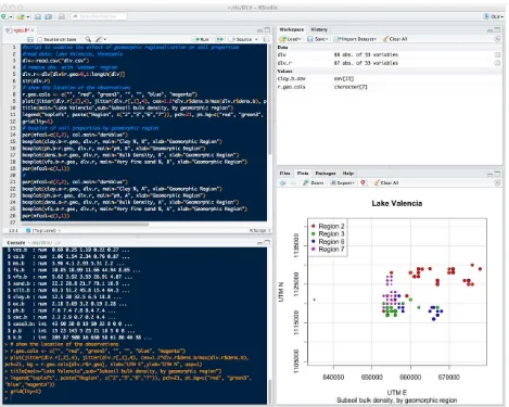
RStudio18 is an excellent cross-platform19 integrated development envi-ronment for R. A screenshot is shown in Figure 1. This environment in-cludes the command line interface, a code editor, output graphs, history, help, workspace contents, and package manager all in one atttractive in-terface. The typical use is: (1) open a script or start a new script; (2) change the working directory to this script’s location; (3) write R code in the script; (4) pass lines of code from the script to the command line interface and evaluate the output; (5) examine any graphs and save for later use.
Figure 1: The RStudio screen
18http://www.rstudio.org/
3.4 TheTinn-Rcode editor
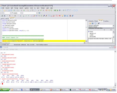
For Windows user, the Tinn-R code editor for Windows20is recommended for those who do not choose to use RStudio. This is tightly integrated with the Windows R GUI, as shown in Figure2. R code is syntax-highlighted and there is extensive help within the editor to select the proper commands and arguments. Commands can be sent directly from the editor to R, or saved in a file and sourced.
Figure 2: The Tinn-R screen, with the R command line interface also visible
3.5 Writing and running scripts
After you have worked out an analysis by typing a sequence of commands, you will probably want to re-run them on edited data, new data, subsets etc. This is easy to do by means ofscripts, which are simply lists of com-mands in a file, written exactly as you would type them at the command
line interface. They are run with the source method. A useful feature of scripts is that you can include comments (lines that begin with the #
character) to explain to yourself or others what the script is doing and why.
Here’s a step-by-step description of how to create and run a simple script which draws two random samples from a normal distribution and com-putes their correlation:21
1. Open a new document in a plain-text editor, i.e., one that does not insert any formatting. Under MS-Windows you can use Notepad or Wordpad; if you are using Tinn-R or RStudio open a new script.
2. Type in the following lines:
x <- rnorm(100, 180, 20) y <- rnorm(100, 180, 20) plot(x, y)
cor.test(x, y)
3. Save the file with the nametest.R, in a convenient directory.
4. Start R (if it’s not already running)
5. In R, select menu commandFile | Source R code ...
6. In the file selection dialog, locate the filetest.Rthat you just saved (changing directories if necessary) and select it; R will run the script.
7. Examine the output.
You can source the file directly from the command line. Instead of steps 5 and 6 above, just typesource("test.R") at the R command prompt (assuming you’ve switched to the directory where you saved the script).
AppendixB contains an example of a more sophisticated script.
For serious work with R you should use a more powerful text editor. The R for Windows, R for Mac OS X and JGR interfaces include built-in edi-tors; another choice on Windows is WinEdt22. And both RStudio (§3.3) and Tinn_R (§3.4) have code editors. For the ultimate in flexibility and power, tryemacs23with the ESS (Emacs Speaks Statistics) module24;
learn-ingemacs is not trivial but rather an investment in a lifetime of efficient
computing.
21What is the expected value of this correlation cofficient?
22http://www.winedt.com/
23http://en.wikipedia.org/wiki/Emacs
3.6 TheRcmdrGUI
The Rcmdr add-on package, written by John Fox of McMaster University,
provides a GUI for common data management and statistical analysis tasks. It is loaded like any other package, with therequiremethod:
> require("Rcmdr")
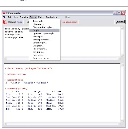
As it is loaded, it starts up in another window, with its own menu system. You can run commands from these menus, but you can also continue to type commands at the R prompt. Figure3shows an R Commander screen shot.
To use Rcmdr, you first import or activate a dataset using one of the commands on Rcmdr’s Data menu; then you can use procedures in the
Statistics, Graphs, andModelsmenus. You can also create and graph
probability distributions with theDistributionsmenu.
When usingRcmdr, observe the commands it formats in response to your menu and dialog box choices. Then you can modify them yourself at the R command line or in a script.
Rcmdr also provides some nice graphics options, including scatterplots
(2D and 3D) where observations can be coloured by a classifying factor.
3.7 Loading optional packages
R starts up with abasepackage, which provides basic statistics and the R language itself. There are a large number of optional packages for specific statistical procedures which can be loaded during a session. Some of these are quite common, e.g.MASS(“Modern Applied Statistics with S” [57]) and
lattice(Trellis graphics [50], §5.2). Others are more specialised, e.g. for
geostatistics and time-series analysis, such asgstat. Some are loaded by default in the base R distribution (see Table4).
If you try to run a method from one of these packages before you load it, you will get the error message
Error: object not found
You can see a list of the packages installed on your system with thelibrary
method with an empty argument:
> library()
To see what functions a package provides, use thelibrarymethod with the named argument. For example, to see what’s in the geostatistical packagegstat:
> library(help=gstat)
To load a package, simply give its name as an argument to the require
method, for example:
> require(gstat)
Once it is loaded, you can get help on any method in the package in the usual way. For example, to get help on the variogram method of the
gstatpackage, once this package has been loaded:
3.8 Sample datasets
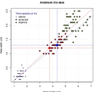
R comes with many example datasets (part of the defaultdatasets pack-age) and most add-in packages also include example datasets. Some of the datasets are classics in a particular application field; an example is theiris dataset used extensively by R A Fisher to illustrate multivariate methods.
To see the list of installed datasets, use thedata method with an empty argument:
> data()
To see the datasets in a single add-in package, use thepackage=argument:
> data(package="gstat")
To load one of the datasets, use its name as the argument to the data
method:
> data(iris)
4 The S language
R is a dialect of the S language, which has a syntax similar to ALGOL-like programming languages such as C, Pascal, and Java. However, S is object-oriented, and makes vector and matrix operations particularly easy; these make it a modern and attractive user and programming environment. In this section we build up from simple to complex commands, and break down their anatomy. A full description of the language is given in theR Language Definition [38]25 and a comprehensive introduction is given in
the Introduction to R [36].26 This section reviews the most outstanding features of S.
All the functions, packages and datasets mentioned in this section (as well as the rest of this note) are indexed (§C) for quick reference.
4.1 Command-line calculator and mathematical operators
The simplest way to use R is as an interactive calculator. For example, to compute the number of radians in one Babylonian degree of a circle:
> 2*pi/360 [1] 0.0174533
As this example shows, S has a few built-in constants, among thempifor the mathematical constantπ. The Euler constanteis not built-in, it must be calculated with theexpfunction asexp(1).
If the assignment operator (explained in the next section) is not present, theexpressionis evaluated and its value is displayed on the console. S has the usual arithmetic operators +, -, *, /, ^ and some less-common ones like%%(modulus) and %/%(integer division). Expressions are evaluated in accordance with the usualoperator precedence; parentheses may be used to change the precedence or make it explicit:
> 3 / 2^2 + 2 * pi [1] 7.03319
> ((3 / 2)^2 + 2) * pi [1] 13.3518
Spaces may be used freely and do not alter the meaning of any S expres-sion.
Commonmathematical functionsare provided asfunctions(see §4.3), in-cludinglog,log10andlog2functions to compute logarithms;expfor ex-ponentiation;sqrtto extract square roots;absfor absolute value;round,
ceiling, floor andtrunc for rounding and related operations;
trigono-metric functions such assin, and inverse trigonometric functions such as
25InRGui, menu commandHelp | Manuals | R Language Manual
asin.
> log(10); log10(10); log2(10) [1] 2.3026
[1] 1 [1] 3.3219 > round(log(10)) [1] 2
> sqrt(5) [1] 2.2361
sin(45 * (pi/180)) [1] 0.7071
> (asin(1)/pi)*180 [1] 90
4.2 Creating new objects: the assignment operator
New objects in the workspace are created with theassignment operator<-, which may also be written as=:
> mu <- 180 > mu = 180
The symbol on the left side is given the value of theexpressionon the right side, creating a new object (or redefining an existing one), here named
mu, in the workspace and assigning it the value of the expression, here the scalar value 180, which is stored as a one-element vector. The two-character symbol<- must be written as two adjacent characters with no spaces..
Now thatmuis defined, it may be printed at the console as an expression:
> print(mu) [1] 180 > mu [1] 180
and it may be used in an expression:
> mu/pi [1] 57.2958
More complex objects may be created:
> s <- seq(10) > s
[1] 1 2 3 4 5 6 7 8 9 10
This creates a new object namedsin the workspace andassignsit the
vec-tor(1 2 ...10). (The syntax ofseq(10)is explained in the next section.)
> (mu <- theta <- pi/2) [1] 1.5708
The final value of the expression, in this case the value of mu, is printed, because the parentheses force the expression to be evaluated as a unit.
Removing objects from the workspace You can remove objects when they are no longer needed with thermfunction:
> rm(s) > s
Error: Object "s" not found
4.3 Methods and their arguments
In the commands <- seq(10), seqis an example of an Smethod, often called a function by analogy with mathematical functions, which has the form:
method.name ( arguments )
Some functions do not need arguments, e.g. to list the objects in the workspace use thelsfunction with anemptyargument list:
> ls()
Note that the empty argument list, i.e. nothing between the(and)is still needed, otherwise the computer code for the function itself is printed.
Optional arguments Most functions haveoptional arguments, which may benamedlike this:
> s <- seq(from=20, to=0, by=-2) > s
[1] 20 18 16 14 12 10 8 6 4 2 0
Named arguments have the formname = value.
Arguments of many functions can also bepositional, that is, their meaning depends on their position in the argument list. The previous command could be written:
> s <- seq(20, 0, by=-2); s
[1] 20 18 16 14 12 10 8 6 4 2 0
The command separator This example shows the use of the;command separator. This allows several commands to be written on one line. In this case the first command computes the sequence and stores it in an object, and the second displays this object. This effect can also be achieved by enclosing the entire expression in parentheses, because then S prints the value of the expression, which in this case is the new object:
> (s <- seq(from=20, to=0, by=-2))
[1] 20 18 16 14 12 10 8 6 4 2 0
Named arguments give more flexibility; this could have been written with names:
> (s <- seq(to=0, from=20, by=-2))
[1] 20 18 16 14 12 10 8 6 4 2 0
but if the arguments are specified only by position the starting value must be before the ending value.
For each function, the list of arguments, both positional and named, and their meaning is given in the on-line help:
> ? seq
Any element or group of elements in a vector can be accessed by using subscripts, very much like in mathematical notation, with the[ ](select array elements) operator:
> samp[1] [1] -1.239197 > samp[1:3]
[1] -1.23919739 0.03765046 2.24047546
> samp[c(1,10)]
[1] -1.239197 9.599777
The notation1:3, using the : sequence operator, produces the sequence from 1 to 3.
The catenate function The notationc(1, 10)is an example of the very useful c orcatenate (“make a chain”) function, which makes a list out of its arguments, in this case the two integers representing the indices of the first and last elements in the vector.
4.4 Vectorized operations and re-cycling
These are calledvectorized operations. As an example of vectorized oper-ations, consider simulating a noisy random process:
> (sample <- seq(1, 10) + rnorm(10))
[1] -0.1878978 1.6700122 2.2756831 4.1454326
[5] 5.8902614 7.1992164 9.1854318 7.5154372
[9] 8.7372579 8.7256403
This adds a random noise (using the rnorm function) with mean 0 and standard deviation 1 (the default) to each of the 10 numbers1..10. Note that both vectors have the same length (10), so they are added element-wise: the first to the first, the second to the second and so forth
If one vector is shorter than the other, its elements arere-cycledas needed:
> (samp <- seq(1, 10) + rnorm(5))
[1] -1.23919739 0.03765046 2.24047546 4.89287818
[5] 4.59977712 3.76080261 5.03765046 7.24047546
[9] 9.89287818 9.59977712
This perturbs the first five numbers in the sequence the same as the sec-ond five.
A simple example of re-cycling is the computation of sample variance di-rectly from the definition, rather than with thevarfunction:
> (sample <- seq(1:8)) [1] 1 2 3 4 5 6 7 8 > (sample - mean(sample))
[1] -3.5 -2.5 -1.5 -0.5 0.5 1.5 2.5 3.5
> (sample - mean(sample))^2
[1] 12.25 6.25 2.25 0.25 0.25 2.25 6.25 12.25
> sum((sample - mean(sample))^2) [1] 42
> sum((sample - mean(sample))^2)/(length(sample)-1) [1] 6
> var(sample) [1] 6
In the expression sample - mean(sample), the mean mean(sample) (a scalar) is being subtracted from sample (a vector). The scalar is a one-element vector; it is shorter than the eight-one-element sample vector, so it is re-cycled: the same mean value is subtracted from each element of the sample vector in turn; the result is a vector of the same length as the sample. Then this entire vector is squared with the^operator; this also is applied element-wise.
Thesumandlengthfunctions are examples of functions thatsummarise
a vector and reduce it to a scalar.
Other functions transform one vector into another. Useful examples are
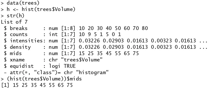
> data(trees) > trees$Volume
[1] 10.3 10.3 10.2 16.4 18.8 19.7 15.6 18.2 22.6 19.9 [11] 24.2 21.0 21.4 21.3 19.1 22.2 33.8 27.4 25.7 24.9 34.5 [22] 31.7 36.3 38.3 42.6 55.4 55.7 58.3 51.5 51.0 77.0 > sort(trees$Volume)
[1] 10.2 10.3 10.3 15.6 16.4 18.2 18.8 19.1 19.7 19.9 [11] 21.0 21.3 21.4 22.2 22.6 24.2 24.9 25.7 27.4 31.7 33.8 [22] 34.5 36.3 38.3 42.6 51.0 51.5 55.4 55.7 58.3 77.0 > rank(trees$Volume)
[1] 2.5 2.5 1.0 5.0 7.0 9.0 4.0 6.0 15.0 10.0
[11] 16.0 11.0 13.0 12.0 8.0 14.0 21.0 19.0 18.0 17.0 22.0
[22] 20.0 23.0 24.0 25.0 28.0 29.0 30.0 27.0 26.0 31.0
Note howrankaverages tied ranks by default; this can be changed by the optionalties.methodargument.
This example also illustrates the $ operator for extracting fields from dataframes; see §4.7.
4.5 Vector and list data structures
Many S functions create complicateddata structures, whose structure must be known in order to use the results in further operations. For example, thesortfunction sorts a vector; when called with the optionalindex=TRUE
argument it also returns the ordering index vector:
> ss <- sort(samp, index=TRUE) > str(ss)
List of 2
$ x : num [1:10] -1.2392 0.0377 2.2405 3.7608 ...
$ ix: int [1:10] 1 2 3 6 5 4 7 8 10 9
This example shows the very importantstr function, which displays the Sstructureof an object.
Lists In this case the object is alist, which in S is an arbitrary collection of other objects. Here the list consists of two objects: a ten-element vector of sorted valuesss$x and a ten-element vector of the indicesss$ix, which are the positions in the original list where the corresponding sorted value was found. We can display just one element of the list if we want:
> ss$ix
[1] 1 2 3 6 5 4 7 8 10 9
This shows the syntax for accessing named components of a data frame or list using the$operator: object $ component, where the$indicates that the component (or field) is to be foundwithinthe named object.
> ss$ix[length(ss$ix)] [1] 9
So the largest value in the sample sequence is found in the ninth position. This example shows howexpressions may contain other expressions, and S evaluates them from the inside-out, just like in mathematics. In this case:
• The innermost expression isss$ix, which is the vector of indices in objectss;
• The next enclosing expression islength(...); thelengthfunction
returns the length of its argument, which is the vector ss$ix (the innermost expression);
• The next enclosing expression is ss$ix[ ...], which converts the result of the expression length(ss$ix)to a subscript and extracts that element from the vectorss$ix.
The result is the array position of the maximum element. We could go one step further to get the actual value of this maximum, which is in the vector
ss$x:
> samp[ss$ix[length(ss$ix)]] [1] 9.599777
but of course we could have gotten this result much more simply with the
maxfunction asmax(ss$x)or evenmax(samp).
4.6 Arrays and matrices
Anarrayis simply a vector with an associateddimensionattribute, to give its shape. Vectors in the mathematical sense are one-dimensional arrays in S;matricesare two-dimensional arrays; higher dimensions are possible.
For example, consider the sample confusion matrix of Congaltonet al.[6], also used as an example by Skidmore [53] and Rossiter [43]:27
Reference Class
A B C D
A 35 14 11 1
Mapped B 4 11 3 0
Class C 12 9 38 4
D 2 5 12 2
This can be entered as a list inrow-major order:
> cm <- c(35,14,11,1,4,11,3,0,12,9,38,4,2,5,12,2) > cm
[1] 35 14 11 1 4 11 3 0 12 9 38 4 2 5 12 2 > dim(cm)
NULL
Initially, the list has no dimensions; these may be added with the dim
function:
> dim(cm) <- c(4, 4) > cm
[,1] [,2] [,3] [,4]
[1,] 35 4 12 2
[2,] 14 11 9 5
[3,] 11 3 38 12
[4,] 1 0 4 2
> dim(cm) [1] 4 4
> attributes(cm) $dim
[1] 4 4
> attr(cm, "dim") [1] 4 4
The attributes function shows any object’s attributes; in this case the
object only has one, its dimension; this can also be read with theattror
dimfunction.
Note that the list was converted to a matrix incolumn-major order, follow-ing the usual mathematical convention that a matrix is made up of column vectors. Thet(transpose) function must be used to specify row-major or-der:
> cm <- t(cm) > cm
[,1] [,2] [,3] [,4]
[1,] 35 14 11 1
[2,] 4 11 3 0
[3,] 12 9 38 4
[4,] 2 5 12 2
A new matrix can also be created with the matrixfunction, which in its simplest form fills a matrix of the specified dimensions (rows, columns) with the value of its first argument:
> (m <- matrix(0, 5, 3)) [,1] [,2] [,3]
[1,] 0 0 0
[2,] 0 0 0
[3,] 0 0 0
[4,] 0 0 0
[5,] 0 0 0
This value may also be a vector:
[1,] 1 2 3
[2,] 4 5 6
[3,] 7 8 9
[4,] 10 11 12
[5,] 13 14 15
> (m <- matrix(1:5, 5, 3)) [,1] [,2] [,3]
[1,] 1 1 1
[2,] 2 2 2
[3,] 3 3 3
[4,] 4 4 4
[5,] 5 5 5
In this last example the shorter vector1:5 is re-cycled as many times as needed to match the dimensions of the matrix; in effect it fills each column with the same sequence.
A matrix element’s rows and column are given by therow andcol func-tions, which are also vectorized and so can be applied to an entire matrix:
> col(m)
[,1] [,2] [,3]
[1,] 1 2 3
[2,] 1 2 3
[3,] 1 2 3
[4,] 1 2 3
[5,] 1 2 3
Thediagfunction applied to an existing matrix extracts its diagonal as a vector:
> (d <- diag(cm))
[1] 35 11 38 2
The diag function applied to a vector creates a square matrix with the vector on the diagonal:
(d <- diag(seq(1:4))) [,1] [,2] [,3] [,4]
[1,] 1 0 0 0
[2,] 0 2 0 0
[3,] 0 0 3 0
[4,] 0 0 0 4
And finallydiagwith a scalar argument creates an indentity matrix of the specified size:
> (d <- diag(3)) [,1] [,2] [,3]
[1,] 1 0 0
[2,] 0 1 0
[3,] 0 0 1
any vector; if matrix multiplication is desired the %*% operator must be used:
> cm*cm
[,1] [,2] [,3] [,4]
[1,] 1225 196 121 1
[2,] 16 121 9 0
[3,] 144 81 1444 16
[4,] 4 25 144 4
> cm%*%cm
[,1] [,2] [,3] [,4]
[1,] 1415 748 857 81
[2,] 220 204 191 16
[3,] 920 629 1651 172
[4,] 238 201 517 54
> cm%*%c(1,2,3,4) [,1]
[1,] 100
[2,] 35
[3,] 160
[4,] 56
As the last example shows,%*%also multiplies matrices and vectors.
A matrix can beinverted with the solve function, usually with little ac-Matrix
inversion curacy loss; in the following example theround function is used to show that we recover an identity matrix:
> solve(cm)
[,1] [,2] [,3] [,4]
[1,] 0.034811530 -0.03680710 -0.004545455 -0.008314856
[2,] -0.007095344 0.09667406 -0.018181818 0.039911308
[3,] -0.020399113 0.02793792 0.072727273 -0.135254989
[4,] 0.105321508 -0.37250554 -0.386363636 1.220066519
> solve(cm)%*%cm
[,1] [,2] [,3] [,4]
[1,] 1.000000e+00 -4.683753e-17 -7.632783e-17 -1.387779e-17
[2,] -1.110223e-16 1.000000e+00 -2.220446e-16 -1.387779e-17
[3,] 1.665335e-16 1.110223e-16 1.000000e+00 5.551115e-17
[4,] -8.881784e-16 -1.332268e-15 -1.776357e-15 1.000000e+00
> round(solve(cm)%*%cm, 10) [,1] [,2] [,3] [,4]
[1,] 1 0 0 0
[2,] 0 1 0 0
[3,] 0 0 1 0
[4,] 0 0 0 1
The samesolvefunction applied to a matrixAand column vector b solves Solving
linear equations
the linear equation b=Ax for x:
> b <- c(1, 2, 3, 4) > (x <- solve(cm, b))
[1] -0.08569845 0.29135255 -0.28736142 3.08148559
> cm %*% x [,1]
[1,] 1
[3,] 3
[4,] 4
Theapplyfunction appliesa function to themargins of a matrix, i.e. the
Applying functions to matrix margins
rows (1) or columns (2). For example, to compute the row and column sums of the confusion matrix, use apply with the sum function as the function to be applied:
> (rsum <- apply(cm, 1, sum)) [1] 61 18 63 21
> (csum <- apply(cm, 2, sum))
[1] 53 39 64 7
These can be used, along with the diag function, to compute the pro-ducer’s and user’s classification accuracies, sincediag(cm)gives the correctly-classified observations:
> (pa <- round(diag(cm)/csum, 2)) [1] 0.66 0.28 0.59 0.29
> (ua <- round(diag(cm)/rsum, 2)) [1] 0.57 0.61 0.60 0.10
The apply function has several variants: lapply and sapply to apply
a user-written or built-in function to each element of a list, tapply to apply a function to groups of values given by some combination of factor levels, and by, a simplified version of this. For example, here is how to standardize a matrix “by hand”, i.e., subtract the mean of each column and divide by the standard deviation of each column:
> apply(cm, 2, function(x) sapply(x, function(i) (i-mean(x))/sd(x)))
[,1] [,2] [,3] [,4]
[1,] 1.381930 -0.10742 -0.24678 -0.689
[2,] -0.087464 1.39642 -0.44420 -0.053
[3,] -0.297377 -0.32225 1.46421 1.431
[4,] -0.997089 -0.96676 -0.77323 -0.689
The outer apply applies a function to the second margin (i.e., columns). The function is defined with thefunctioncommand.
The structure is clearer if braces are used (optional here because each function only has one command) and the command is written on several lines to show the matching braces and parentheses:
> apply(cm, 2, function(x)
+ {
+ sapply(x, function(i)
+ { (i-mean(x))/sd(x)
+ } # end function
+ ) # end sapply
+ } # end function
+ ) # end apply
“scale a matrix” function, which in addition to scaling a matrix column-wise (with or without centring, with or without scaling) returns attributes showing the central values (means) and scaling values (standard devia-tions) used:
> scale(cm)
[,1] [,2] [,3] [,4]
[1,] 1.381930 -0.10742 -0.24678 -0.689
[2,] -0.087464 1.39642 -0.44420 -0.053
[3,] -0.297377 -0.32225 1.46421 1.431
[4,] -0.997089 -0.96676 -0.77323 -0.689 attr(,"scaled:center")
[1] 15.25 4.50 15.75 5.25
attr(,"scaled:scale")
[1] 14.2916 4.6547 15.1959 4.7170
There are also functions to compute the determinant (det), eigenvalues Other
matrix functions
and eigenvectors (eigen), the singular value decomposition (svd), the QR decomposition (qr), and the Choleski factorization (chol); these use long-standing numerical codes from LINPACK, LAPACK, and EISPACK.
4.7 Data frames
The fundamental S data structure for statistical modelling is the data frame. This can be thought of as a matrix where the rows are cases, calledobservationsby S (whether or not they were field observations), and the columns are the variables. In standard database terminology, these are records and fields, respectively. Rows are generally accessed by the row number (although they can have names), and columns by the vari-ablename(although they can also be accessed by number). A data frame can also be considerd a list whose members are the fields; these can be accessed with the[[ ]](list access) operator.
Sample data R comes with many example datasets (§3.8) organized as data frames; let’s load one (trees) and examine its structure and several ways to access its components:
> ?trees > data(trees) > str(trees)
`data.frame': 31 obs. of 3 variables:
$ Girth : num 8.3 8.6 8.8 10.5 10.7 10.8 11 ...
$ Height: num 70 65 63 72 81 83 66 75 80 75 ...
$ Volume: num 10.3 10.3 10.2 16.4 18.8 19.7 ...
The help text tells us that this data set contains measurements of the girth (diameter in inches28, measured at 4.5 ft29height), height (feet) and timber
281 inch=2.54 cm
volume (cubic feet30) in 31 felled black cherry trees. The data frame has 31 observations (rows, cases, records) each of which has three variables (columns, attributes, fields). Their names can be retrieved or changed by
thenames function. For example, to name the fieldsVar.1,Var.2etc. we
could use thepastefunction to build the names into a list and then assign this list to the names attribute of the data frame:
> (saved.names <- names(trees)) [1] "Girth" "Height" "Volume"
> (names(trees) <- paste("Var", 1:dim(trees)[2], sep=".")) [1] "Var.1" "Var.2" "Var.3''
> names(trees)[1] <- "Perimeter" > names(trees)
[1] "Perimeter" "V.2" "V.3" > (names(trees) <- saved.names) [1] "Girth" "Height" "Volume" > rm(saved.names)
Note in thepaste function how the shorter vector"Var"wasre-cycled to match the longer vector 1:dim(trees)[2]. This was just an example of how to name fields; at the end we restore the original names, which we had saved in a variable which, since we no longer need it, we remove from the workspace with thermfunction.
The data frame can accessed various ways:
> # most common: by field name
> trees$Height
[1] 70 65 63 72 81 83 66 75 80 75 79 76 76 69 [15] 75 74 85 86 71 64 78 80 74 72 77 81 82 80 [29] 80 80 87
> # the result is a vector, can select elements of it
> trees$Height[1:5] [1] 70 65 63 72 81
> # but this is also a list element
> trees[[2]]
[1] 70 65 63 72 81 83 66 75 80 75 79 76 76 69 [15] 75 74 85 86 71 64 78 80 74 72 77 81 82 80 [ 29] 80 80 87
> trees[[2]][1:5] [1] 70 65 63 72 81
> # as a matrix, first by row....
> trees[1,]
Girth Height Volume
1 8.3 70 10.3
> # ... then by column
> trees[,2]
> trees[[2]]
[1] 70 65 63 72 81 83 66 75 80 75 79 76 76 69 [15] 75 74 85 86 71 64 78 80 74 72 77 81 82 80 [ 29] 80 80 87
> # get one element
> trees[1,2] [1] 70
301 ft3
> trees[1,"Height"] [1] 70
> trees[1,]$Height [1] 70
The forms like$Heightuse the$ operator to select anamed fieldwithin the frame. The forms like[1, 2]show that this is just a matrix with col-umn names, leading to forms like trees[1,"Height"]. The forms like
trees[1,]$Heightshow that each row (observation, case) can be
consid-ered a list with named items. The forms liketrees[[2]] show that the data frame is also a list whose elements can be accessed with the[[ ]]
operator.
Attaching data frames to the search path To simplify access to named columns of data frames, S provides an attach function that makes the names visible in the outer namespace:
> attach(trees) > Height[1:5] [1] 70 65 63 72 81
Building a data frame S provides thedata.framefunction for creating data frames from smaller objects, usually vectors. As a simple example, suppose the number of trees in a plot has been measured at five plots in each of two transects on a regular spacing. We enter the x-coördinate as one list, the y-coördinate as another, and the number of trees in each plot as the third:
> x <- rep(seq(182,183, length=5), 2)*1000 > y <- rep(c(381000, 310300), 5)
> n.trees <- c(10, 12, 22, 4, 12, 15, 7, 18, 2, 16) > (ds <- data.frame(x, y, n.trees))
x y n.trees
1 182000 381000 10
2 182250 310300 12
3 182500 381000 22
4 182750 310300 4
5 183000 381000 12
6 182000 310300 15
7 182250 381000 7
8 182500 310300 18
9 182750 381000 2
10 183000 310300 16
Note the use of the rep function to repeat a sequence. Also note that an arithmetic expression (in this case* 1000) can be applied to an entire vector (in this caserep(seq(182,183, length=5), 2)).
Adding rows to a data frame Therbind(“row bind”) function is used to add rows to a data frame, and to combine two data frames with the same structure. For example, to add one more trees to the data frame:
> (ds <- rbind(ds, c(183500, 381000, 15)))
x y n.trees
1 182000 381000 10
2 182250 310300 12
3 182500 381000 22
4 182750 310300 4
5 183000 381000 12
6 182000 310300 15
7 182250 381000 7
8 182500 310300 18
9 182750 381000 2
10 183000 310300 16
11 183500 381000 15
This can also be accomplished by directly assigning to the next row:
> ds[12,] <- c(183400, 381200, 18) > ds
x y n.trees
1 182000 381000 10
2 182250 310300 12
3 182500 381000 22
4 182750 310300 4
5 183000 381000 12
6 182000 310300 15
7 182250 381000 7
8 182500 310300 18
9 182750 381000 2
10 183000 310300 16
11 183500 381000 12
12 183400 381200 18
Adding fields to a data frame A vector with the same number of rows as an existing data frame may be added to it with thecbind(“column bind”) function. For example, we could compute a height-to-girth ratio for the trees (a measure of a tree’s shape) and add it as a new field to the data frame; we illustrate this with the trees example dataset introduced in §4.7:
> attach(trees)
> HG.Ratio <- Height/Girth; str(HG.Ratio)
num [1:31] 8.43 7.56 7.16 6.86 7.57 ...
> trees <- cbind(trees, HG.Ratio); str(trees)
`data.frame': 31 obs. of 4 variables:
$ Girth : num 8.3 8.6 8.8 10.5 10.7 10.8 ...
$ Height : num 70 65 63 72 81 83 66 75 80 75 ...
$ Volume : num 10.3 10.3 10.2 16.4 18.8 19.7 ...
$ HG.Ratio: num 8.43 7.56 7.16 6.86 7.57 ..
Note that this new field is not visible in an attached frame; the frame must be detached (with thedetachfunction) and re-attached:
> summary(HG.Ratio)
Error: Object "HG.Ratio" not found > detach(trees); attach(trees) > summary(HG.Ratio)
Min. 1st Qu. Median Mean 3rd Qu. Max.
4.22 4.70 6.00 5.99 6.84 8.43
Sorting a data frame This is most easily accomplished with the order
function, naming the field(s) on which to sort, and then using the returned indices to extract rows of the data frame in sorted order:
> trees[order(trees$Height, trees$Girth),] Girth Height Volume
3 8.8 63 10.2
20 13.8 64 24.9
2 8.6 65 10.3
...
4 10.5 72 16.4
24 16.0 72 38.3
16 12.9 74 22.2
23 14.5 74 36.3
...
18 13.3 86 27.4
31 20.6 87 77.0
Note that the trees are first sorted by height, then any ties in height are sorted by girth.
4.8 Factors
Some variables arecategorical: they can take only a defined set of values. In S these are called factors and are of two types: unordered (nominal) andordered (ordinal). An example of the first is a soil type, of the second soil structure grade, from “none” through “weak” to “strong” and “very strong”; there is a natural order in the second case but not in the first. Many analyses in R depend on factors being correctly identified; some such astable(§4.15) only work with categorical variables.
Factors are defined with thefactorandorderedfunctions. They may be converted from existing character or numeric vectors with theas.factor
and as.ordered function; these are often used after data import if the
read.tableor related functions could not correctly identify factors; see
§6.3for an example. The levels of an existing factor are extracted with the
levelsfunction.
> student <- rep(1:3, 3)
> score <- c(9, 6.5, 8, 8, 7.5, 6, 9.5, 8, 7) > tests <- data.frame(cbind(student, score)) > str(tests)
`data.frame': 9 obs. of 2 variables:
$ student: num 1 2 3 1 2 3 1 2 3
$ score : num 9 6.5 8 8 7.5 6 9.5 8 7
We have the data but the student is just listed by a number; the table
function won’t work and if we try to predict the score from the student using thelmfunction (see §4.17) we get nonsense:
> lm(score ~ student, data=tests) Coefficients:
(Intercept) student
9.556 -0.917
The problem is that the student is considered as a continuous variable when in fact it is a factor. We do much better if we make the appropriate conversion:
> tests$student <- as.factor(tests$student) > str(tests)
`data.frame': 9 obs. of 2 variables:
$ student: Factor w/ 3 levels "1","2","3": 1 2 3 1 2 3 1 2 3
$ score : num 9 6.5 8 8 7.5 6 9.5 8 7
> lm(score ~ student, data=tests) Coefficients:
(Intercept) student2 student3
8.83 -1.50 -1.83
This is a meaningful one-way linear model, showing the difference in mean scores of students 2 and 3 from student 1 (the intercept).
Factor names can be any string; so to be more descriptive we could have assigned names with thelabelsargument to thefactorfunction:
> tests$student <- factor(tests$student, labels=c("Harley", "Doyle", "JD")) > str(tests)
'data.frame': 9 obs. of 2 variables:
$ student: Factor w/ 3 levels "Harley","Doyle",..: 1 2 3 1 2 3 1 2 3
$ score : num 9 6.5 8 8 7.5 6 9.5 8 7
> table(tests) score
student 6 6.5 7 7.5 8 9 9.5
Harley 0 0 0 0 1 1 1
Doyle 0 1 0 1 1 0 0
JD 1 0 1 0 1 0 0
An existing factor can berecoded with an additional call to factor and different labels:
> tests$student <- factor(tests$student, labels=c("John", "Paul", "George")) > str(tests)
$ student: Factor w/ 3 levels "John","Paul",..: 1 2 3 1 2 3 1 2 3
$ score : num 9 6.5 8 8 7.5 6 9.5 8 7
> table(tests) score
student 6 6.5 7 7.5 8 9 9.5
John 0 0 0 0 1 1 1
Paul 0 1 0 1 1 0 0
George 1 0 1 0 1 0 0
The levels have the same internal numbers but different labels. This use
offactorwith the optional labelsargument does not change the order
of the factors, which will be presented in the original order. If for example we want to present them alphabetically, we need to re-order the levels, ex-tracting them with thelevelsfunction in the order we want (as indicated by subscripts), and then setting these (in the new order) with the optional
levelsargument tofactor:
> tests$student <- factor(tests$student, levels=levels(tests$student)[c(3,1,2)]) > str(tests)
'data.frame': 9 obs. of 2 variables:
$ student: Factor w/ 3 levels "George","John",..: 2 3 1 2 3 1 2 3 1
$ score : num 9 6.5 8 8 7.5 6 9.5 8 7
> table(tests) score
student 6 6.5 7 7.5 8 9 9.5
George 1 0 1 0 1 0 0
John 0 0 0 0 1 1 1
Paul 0 1 0 1 1 0 0
Now the three students are presented in alphabetic order, because the underlying codes have been re-ordered. Thecarpackage contains a useful
recodefunction which also allows grouping of factors.
Factors require special care in statistical models; see §4.17.1.
4.9 Selecting subsets
We often need to examine subsets of our data, for example to perform a separate analysis for several strata defined by some factor, or to exclude outliers defined by some criterion.
Selecting known elements If we know the observation numbers, we sim-ply name them as the first subscript, using the[ ](select array elements) operator:
> trees[1:3,]
Girth Height Volume
1 8.3 70 10.3
2 8.6 65 10.3
3 8.8 63 10.2
1 8.3 70 10.3
3 8.8 63 10.2
5 10.7 81 18.8
> trees[seq(1, 31, by=10),] Girth Height Volume
1 8.3 70 10.3
11 11.3 79 24.2
21 14.0 78 34.5
31 20.6 87 77.0
Anegativesubscript in this syntaxexcludesthe named rows and includes all the others:
> trees[-(1:27),] Girth Height Volume
28 17.9 80 58.3
29 18.0 80 51.5
30 18.0 80 51.0
31 20.6 87 77.0
Selecting with a logical expression The simplest way to select subsets is with alogical expressionon therow subscript which gives the criterion. For example, in the trees example dataset introduced in §4.7, there is only one tree with volume greater than 58 cubic feet, and it is substantially larger; we can see these in order with thesortfunction:
> attach(trees) > sort(Volume)
[1] 10.2 10.3 10.3 15.6 16.4 18.2 18.8 19.1 19.7
[11] 19.9 21.0 21.3 21.4 22.2 22.6 24.2 24.9 25.7
[21] 27.4 31.7 33.8 34.5 36.3 38.3 42.6 51.0 51.5
[31] 55.4 55.7 58.3 77.0
To analyze the data without this “unusual” tree, we use a logical expression to select rows (observations), here using the<(less than)logical compara-ison operator, and then the[ ](select array elements) operator to extract the array elements that are selected:
> tr <- trees[Volume < 60,]
Note that there is no condition for the second subscript, so all columns are selected.
To make a list of the observation numbers where a certain condition is met, use thewhichfunction:
> which(trees$Volume > 60) [1] 31
> trees[which(trees$Volume > 60),] Girth Height Volume
Logical expressions may be combined withlogical operatorssuch as& (log-ical AND) and|(logical OR), and their truth sense inverted with! (logical NOT). For example, to select trees with volumes between 20 and 40 cubic feet:
> tr <- trees[Volume >=20 & Volume <= 40,]
Note that&, like S arithmetical operators, isvectorized, i.e. it operates on each pair of elements of the two logical vectors separately.
Parentheses should be used if you are unclear about operator precedence. Since the logical comparaison operators (e.g.>=) have precedence over bi-nary logical operators (e.g.&), the previous expression is equivalent to:
> tr <- trees[(Volume >=20) & (Volume <= 40),]
Another way to select elements is to make asubset, with thesubset func-tion:
> (tr.small <- subset(trees, Volume < 18)) Girth Height Volume
1 8.3 70 10.3
2 8.6 65 10.3
3 8.8 63 10.2
4 10.5 72 16.4
7 11.0 66 15.6
Selecting random elements of an array Random elements of a vector can be selected with thesamplefunction:
> trees[sort(sample(1:dim(trees)[1], 5)), ] Girth Height Volume
13 11.4 76 21.4
18 13.3 86 27.4
22 14.2 80 31.7
23 14.5 74 36.3
26 17.3 81 55.4
Each call tosamplewill give a different result.
By default sampling is without replacement, so the same element can not be selected more than once; for sampling with replacement use the
replace=Toptional argument.
In this example, the commanddim(trees)uses thedimfunction to give the dimensions of the data frame (rows and columns); the first element of this two-element list is the number of rows:dim(trees)[1].