Physical Metallurgy and
Advanced Materials
Seventh edition
R. E. Smallman,
CBE, DSc, FRS, FREng, FIMMMA. H. W. Ngan,
PhD, FIMMM, CSci, CEngAMSTERDAM•BOSTON•HEIDELBERG•LONDON•NEW YORK•OXFORD PARIS•SAN DIEGO•SAN FRANCISCO•SINGAPORE•SYDNEY•TOKYO
30 Corporate Drive, Suite 400, Burlington, MA 01803
Seventh edition 2007
Copyright © 2007, R. E. Smallman and A. H. W. Ngan. Published by Elsevier Ltd. All rights reserved.
The right of R. E. Smallman and A. H. W. Ngan to be identified as the authors of this work has been asserted in accordance with the Copyright, Designs and Patents Act 1988
No part of this publication may be reproduced, stored in a retrieval system, or transmitted in any form or by any means electronic, mechanical, photocopying, recording or otherwise without the prior written permission of the publisher
Permissions may be sought directly from Elsevier’s Science & Technology Rights Department in Oxford, UK: phone (+44) (0) 1865 843830; fax (+44) (0) 1865 853333; email: [email protected]. Alternatively you can submit your request online by visiting the Elsevier website at http://elsevier.com/locate/permissions, and selecting Obtaining permission to use Elsevier material
Notice
No responsibility is assumed by the publisher for any injury and/or damage to persons or property as a matter of products liability, negligence or otherwise, or from any use or operation of any methods, products, instructions or ideas contained in the material herein. Because of rapid advances in the medical sciences, in particular, independent verification of diagnoses and drug dosages should be made
British Library Cataloguing in Publication Data
A catalogue record for this book is available from the British Library
Library of Congress Cataloging-in-Publication Data
A catalog record for this book is available from the Library of Congress
ISBN: 978 0 7506 6906 1
For information on all Butterworth-Heinemann publications visit our website at http://books.elsevier.com
Preface xiii
About the authors xv
Acknowledgments xvi
Illustration credits xvii
Chapter 1 Atoms and atomic arrangements 1
1.1 The realm of materials science 1
1.2 The free atom 1
1.2.1 The four electron quantum numbers 1
1.2.2 Nomenclature for the electronic states 2
1.3 The Periodic Table 5
1.4 Interatomic bonding in materials 9
1.5 Bonding and energy levels 13
1.6 Crystal lattices and structures 15 1.7 Crystal directions and planes 16
1.8 Stereographic projection 20
1.9 Selected crystal structures 24
1.9.1 Pure metals 24
1.9.2 Diamond and graphite 29
1.9.3 Coordination in ionic crystals 30
1.9.4 AB-type compounds 33
Chapter 2 Phase equilibria and structure 37
2.1 Crystallization from the melt 37
2.1.1 Freezing of a pure metal 37
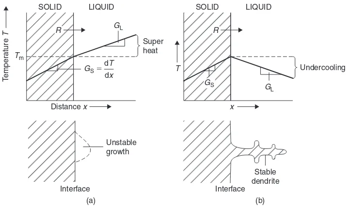
2.1.2 Plane-front and dendritic solidification at a cooled surface 39
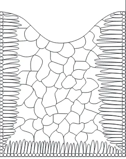
2.1.3 Forms of cast structure 40
2.1.4 Gas porosity and segregation 42
2.1.5 Directional solidification 43
2.1.6 Production of metallic single crystals for research 44
2.2 Principles and applications of phase diagrams 45
2.2.1 The concept of a phase 45
2.2.2 The Phase Rule 46
2.2.3 Stability of phases 47
2.2.4 Two-phase equilibria 51
2.2.5 Three-phase equilibria and reactions 58
2.2.6 Intermediate phases 62
2.2.7 Limitations of phase diagrams 63
2.2.8 Some key phase diagrams 64
2.2.9 Ternary phase diagrams 67
2.3 Principles of alloy theory 74
2.3.1 Primary substitutional solid solutions 74
2.3.2 Interstitial solid solutions 80
2.3.3 Types of intermediate phases 81
2.3.4 Order–disorder phenomena 85
2.4 The mechanism of phase changes 86
2.4.1 Kinetic considerations 86
2.4.2 Homogeneous nucleation 88
2.4.3 Heterogeneous nucleation 90
2.4.4 Nucleation in solids 91
Chapter 3 Crystal defects 95
3.1 Types of imperfection 95
3.2 Point defects 96
3.2.1 Point defects in metals 96
3.2.2 Point defects in non-metallic crystals 99
3.2.3 Irradiation of solids 101
3.2.4 Point defect concentration and annealing 104
3.3 Line defects 107
3.3.1 Concept of a dislocation 107
3.3.2 Edge and screw dislocations 108
3.3.3 The Burgers vector 108
3.3.4 Mechanisms of slip and climb 109
3.3.5 Strain energy associated with dislocations 113
3.3.6 Dislocations in ionic structures 117
3.4 Planar defects 117
3.4.1 Grain boundaries 117
3.4.2 Twin boundaries 120
3.4.3 Extended dislocations and stacking faults in close-packed crystals 121
3.5 Volume defects 128
3.5.1 Void formation and annealing 128
3.5.2 Irradiation and voiding 128
3.5.3 Voiding and fracture 129
3.6 Defect behavior in common crystal structures 129
3.6.1 Dislocation vector diagrams and the Thompson tetrahedron 129
3.6.2 Dislocations and stacking faults in fcc structures 130
3.6.3 Dislocations and stacking faults in cph structures 138
3.6.4 Dislocations and stacking faults in bcc structures 142
3.6.5 Dislocations and stacking faults in ordered structures 144
3.7 Stability of defects 147
3.7.1 Dislocation loops 147
3.7.2 Voids 150
3.7.3 Nuclear irradiation effects 152
Chapter 4 Characterization and analysis 161
4.1 Tools of characterization 161
4.2 Light microscopy 162
4.2.1 Basic principles 162
4.2.2 Selected microscopical techniques 165
4.3 X-ray diffraction analysis 169
4.3.1 Production and absorption of X-rays 169
4.3.2 Diffraction of X-rays by crystals 171
4.3.3 X-ray diffraction methods 172
4.4 Analytical electron microscopy 184
4.4.1 Interaction of an electron beam with a solid 184
4.4.2 The transmission electron microscope (TEM) 185
4.4.3 The scanning electron microscope 187
4.4.4 Theoretical aspects of TEM 190
4.4.5 Chemical microanalysis 196
4.4.6 Electron energy-loss spectroscopy (EELS) 202
4.4.7 Auger electron spectroscopy (AES) 203
4.5 Observation of defects 204
4.5.1 Etch pitting 204
4.5.2 Dislocation decoration 205
4.5.3 Dislocation strain contrast in TEM 205
4.5.4 Contrast from crystals 207
4.5.5 Imaging of dislocations 208
4.5.6 Imaging of stacking faults 209
4.5.7 Application of dynamical theory 210
4.5.8 Weak-beam microscopy 212
4.6 Scanning probe microscopy 214
4.6.1 Scanning tunneling microscopy (STM) 215
4.6.2 Atomic force microscopy (AFM) 219
4.6.3 Applications of SPM 221
4.6.4 Nanoindentation 222
4.7 Specialized bombardment techniques 230
4.7.1 Neutron diffraction 230
4.7.2 Synchrotron radiation studies 232
4.7.3 Secondary ion mass spectrometry (SIMS) 233
4.8 Thermal analysis 234
4.8.1 General capabilities of thermal analysis 234
4.8.2 Thermogravimetric analysis 234
4.8.3 Differential thermal analysis 235
4.8.4 Differential scanning calorimetry 236
Chapter 5 Physical properties 239
5.1 Introduction 239
5.2 Density 239
5.3 Thermal properties 240
5.3.1 Thermal expansion 240
5.3.2 Specific heat capacity 242
5.3.3 The specific heat curve and transformations 243
5.3.4 Free energy of transformation 244
5.4 Diffusion 245
5.4.1 Diffusion laws 245
5.4.2 Mechanisms of diffusion 249
5.4.3 Factors affecting diffusion 250
5.5 Anelasticity and internal friction 251
5.6 Ordering in alloys 254
5.6.1 Long-range and short-range order 254
5.6.2 Detection of ordering 255
5.6.3 Influence of ordering on properties 259
5.7 Electrical properties 260
5.7.2 Semiconductors 264
5.7.3 Hall effect 267
5.7.4 Superconductivity 269
5.7.5 Oxide superconductors 272
5.8 Magnetic properties 273
5.8.1 Magnetic susceptibility 273
5.8.2 Diamagnetism and paramagnetism 274
5.8.3 Ferromagnetism 275
5.8.4 Magnetic alloys 277
5.8.5 Anti-ferromagnetism and ferrimagnetism 281
5.9 Dielectric materials 282
5.9.1 Polarization 282
5.9.2 Capacitors and insulators 283
5.9.3 Piezoelectric materials 283
5.9.4 Pyroelectric and ferroelectric materials 283
5.10 Optical properties 284
5.10.1 Reflection, absorption and transmission effects 284
5.10.2 Optical fibers 285
5.10.3 Lasers 286
5.10.4 Ceramic ‘windows’ 287
5.10.5 Electro-optic ceramics 287
Chapter 6 Mechanical properties I 289
6.1 Mechanical testing procedures 289
6.1.1 Introduction 289
6.1.2 The tensile test 289
6.1.3 Indentation hardness testing 292
6.1.4 Impact testing 292
6.1.5 Creep testing 292
6.1.6 Fatigue testing 293
6.2 Elastic deformation 294
6.3 Plastic deformation 297
6.3.1 Slip and twinning 297
6.3.2 Resolved shear stress 298
6.3.3 Relation of slip to crystal structure 300
6.3.4 Law of critical resolved shear stress 300
6.3.5 Multiple slip 301
6.3.6 Relation between work hardening and slip 303
6.4 Dislocation behavior during plastic deformation 303
6.4.1 Dislocation mobility 303
6.4.2 Variation of yield stress with temperature and strain rate 304
6.4.3 Dislocation source operation 306
6.4.4 Discontinuous yielding 310
6.4.5 Yield points and crystal structure 312
6.4.6 Discontinuous yielding in ordered alloys 314
6.4.7 Solute–dislocation interaction 315
6.4.8 Dislocation locking and temperature 318
6.4.9 Inhomogeneity interaction 320
6.4.10 Kinetics of strain ageing 320
6.4.11 Influence of grain boundaries on plasticity 321
6.5 Mechanical twinning 326
6.5.1 Crystallography of twinning 326
6.5.2 Nucleation and growth of twins 327
6.5.3 Effect of impurities on twinning 329
6.5.4 Effect of prestrain on twinning 329
6.5.5 Dislocation mechanism of twinning 329
6.5.6 Twinning and fracture 330
6.6 Strengthening and hardening mechanisms 330
6.6.1 Point defect hardening 330
6.6.2 Work hardening 332
6.6.3 Development of preferred orientation 341
6.7 Macroscopic plasticity 345
6.7.1 Tresca and von Mises criteria 345
6.7.2 Effective stress and strain 347
6.8 Annealing 348
6.8.1 General effects of annealing 348
6.8.2 Recovery 349
6.8.3 Recrystallization 351
6.8.4 Grain growth 355
6.8.5 Annealing twins 358
6.8.6 Recrystallization textures 360
6.9 Metallic creep 361
6.9.1 Transient and steady-state creep 361
6.9.2 Grain boundary contribution to creep 365
6.9.3 Tertiary creep and fracture 367
6.9.4 Creep-resistant alloy design 368
6.10 Deformation mechanism maps 370
6.11 Metallic fatigue 371
6.11.1 Nature of fatigue failure 371
6.11.2 Engineering aspects of fatigue 372
6.11.3 Structural changes accompanying fatigue 375
6.11.4 Crack formation and fatigue failure 378
6.11.5 Fatigue at elevated temperatures 381
Chapter 7 Mechanical properties II – Strengthening and toughening 385
7.1 Introduction 385
7.2 Strengthening of non-ferrous alloys by heat treatment 385
7.2.1 Precipitation hardening of Al–Cu alloys 385
7.2.2 Precipitation hardening of Al–Ag alloys 391
7.2.3 Mechanisms of precipitation hardening 394
7.2.4 Vacancies and precipitation 399
7.2.5 Duplex ageing 403
7.2.6 Particle coarsening 404
7.2.7 Spinodal decomposition 407
7.3 Strengthening of steels by heat treatment 409
7.3.1 Time–temperature–transformation diagrams 409
7.3.2 Austenite–pearlite transformation 411
7.3.3 Austenite–martensite transformation 414
7.3.4 Austenite–bainite transformation 420
7.3.5 Tempering of martensite 420
7.4 Fracture and toughness 423
7.4.1 Griffith microcrack criterion 423
7.4.2 Fracture toughness 426
7.4.3 Cleavage and the ductile–brittle transition 429
7.4.4 Factors affecting brittleness of steels 431
7.4.5 Hydrogen embrittlement of steels 432
7.4.6 Intergranular fracture 434
7.4.7 Ductile failure 434
7.4.8 Rupture 436
7.4.9 Voiding and fracture at elevated temperatures 436
7.4.10 Fracture mechanism maps 438
7.4.11 Crack growth under fatigue conditions 439
7.5 Atomistic modeling of mechanical behavior 440
7.5.1 Multiscale modeling 441
7.5.2 Atomistic simulations of defects 442
Chapter 8 Advanced alloys 447
8.1 Introduction 447
8.2 Commercial steels 447
8.2.1 Plain carbon steels 447
8.2.2 Alloy steels 448
8.2.3 Maraging steels 450
8.2.4 High-strength low-alloy (HSLA) steels 450
8.2.5 Dual-phase (DP) steels 451
8.2.6 Mechanically alloyed (MA) steels 454
8.2.7 Designation of steels 455
8.3 Cast irons 455
8.4 Superalloys 458
8.4.1 Basic alloying features 458
8.4.2 Nickel-based superalloy development 460
8.4.3 Dispersion-hardened superalloys 462
8.5 Titanium alloys 462
8.5.1 Basic alloying and heat-treatment features 462
8.5.2 Commercial titanium alloys 465
8.5.3 Processing of titanium alloys 467
8.6 Structural intermetallic compounds 467
8.6.1 General properties of intermetallic compounds 467
8.6.2 Nickel aluminides 468
8.6.3 Titanium aluminides 470
8.6.4 Other intermetallic compounds 473
8.7 Aluminum alloys 474
8.7.1 Designation of aluminum alloys 474
8.7.2 Applications of aluminum alloys 475
8.7.3 Aluminum–lithium alloys 475
8.7.4 Processing developments 477
Chapter 9 Oxidation, corrosion and surface treatment 481
9.1 The engineering importance of surfaces 481
9.2 Metallic corrosion 481
9.2.1 Oxidation at high temperatures 481
9.3 Surface engineering 500
9.3.1 The coating and modification of surfaces 500
9.3.2 Surface coating by vapor deposition 501
9.3.3 Surface coating by particle bombardment 505
9.3.4 Surface modification with high-energy beams 506
9.4 Thermal barrier coatings 508
9.5 Diamond-like carbon 508
9.6 Duplex surface engineering 508
Chapter 10 Non-metallics I – Ceramics, glass, glass-ceramics 513
10.1 Introduction 513
10.2 Sintering of ceramic powders 513
10.2.1 Powdering and shaping 516
10.2.2 Sintering 517
10.3 Some engineering and commercial ceramics 519
10.3.1 Alumina 519
10.3.2 Silica 519
10.3.3 Silicates 520
10.3.4 Perovskites, titanates and spinels 522
10.3.5 Silicon carbide 523
10.3.6 Silicon nitride 523
10.3.7 Sialons 524
10.3.8 Zirconia 526
10.4 Glasses 528
10.4.1 Structure and characteristics 528
10.4.2 Processing and properties 530
10.4.3 Glass-ceramics 533
10.5 Carbon 534
10.5.1 Diamond 535
10.5.2 Graphite 536
10.5.3 Fullerenes and related nanostructures 537
10.6 Strength of ceramics and glasses 540
10.6.1 Strength measurement for brittle materials 540
10.6.2 Statistical nature and size dependence of strength 541
10.6.3 Stress corrosion cracking of ceramics and glasses 543
10.7 A case study: thermal protection system in space shuttle orbiter 545
Chapter 11 Non-metallics II – Polymers, plastics, composites 549
11.1 Polymer molecules 549
11.2 Molecular weight 549
11.3 Polymer shape and structure 552
11.4 Polymer crystallinity 553
11.5 Polymer crystals 555
11.6 Mechanical behavior 557
11.6.1 Deformation 557
11.6.2 Viscoelasticity 559
11.6.3 Fracture 560
11.7 Plastics and additives 562
11.8 Polymer processing 562
11.9 Electrical properties 564
11.10 Composites 565
11.10.2 Fiber-reinforced composites 566
11.10.3 Fiber orientations 569
11.10.4 Influence of fiber length 570
11.10.5 Composite fibers 571
11.10.6 Polymer–matrix composites (PMCs) 574
11.10.7 Metal–matrix composites (MMCs) 576
11.10.8 Ceramic–matrix composites (CMCs) 578
Chapter 12 Case examination of biomaterials, sports materials and nanomaterials 583
12.1 Introduction 583
12.2 Biomaterials 583
12.2.1 Introduction and bio-requirements 583
12.2.2 Introduction to bone and tissue 584
12.2.3 Case consideration of replacement joints 587
12.2.4 Biomaterials for heart repair 590
12.2.5 Reconstructive surgery 593
12.2.6 Ophthalmics 594
12.2.7 Dental materials 595
12.2.8 Drug delivery systems 597
12.3 Sports materials 598
12.3.1 Introduction 598
12.3.2 Golf equipment 598
12.3.3 Tennis equipment 600
12.3.4 Bicycles 600
12.3.5 Skiing materials 603
12.3.6 Archery 603
12.3.7 Fencing foils 605
12.3.8 Sports protection 606
12.4 Materials for nanotechnology 607
12.4.1 Introduction 607
12.4.2 Nanoparticles 608
12.4.3 Fullerenes and nanotubes 609
12.4.4 Quantum wells, wires and dots 610
12.4.5 Bulk nanostructured solids 612
12.4.6 Mechanical properties of small material volumes 613
12.4.7 Bio-nanotechnology 619
Numerical answers to problems 623
Appendix 1 SI units 627
Appendix 2 Conversion factors, constants and physical data 629
Physical Metallurgy andAdvanced Materialshas evolved from the earlier editions ofModern Physical Metallurgy(1962, 1970, 1985) and later editions of Modern Physical Metallurgy and Materials Engineering(1995, 1999). The present treatment contains much of the previous editions and follows the same overall philosophy and aims. It has, however, been updated again in both presentation and content. Additions have been made to almost every chapter, which now include a number of worked examples in the text to illustrate and emphasize a particular aspect of the subject. At the end of each chapter there is a set of questions, most of which are numerical. These are included to give the reader an opportunity to apply the scientific background presented in the chapter, but also to emphasize important material properties, e.g. elastic moduli, atomic dimensions, etc. The solutions to these problems are worked out in a Solutions Manual, which may be obtained from Elsevier by teachers and lecturers who use the book.
To keep the book a manageable size some text from the previous edition has been omitted together with associated diagrams, and some of the text has been totally recast in a different format. The early chapters are predominantly directed towards metals (physical metallurgy) but the principles are equally relevant to non-metals, which are specifically dealt with in the later chapters. Characterization using X-rays, electron microscopy, etc. is important to all areas of materials and several new techniques such as scanning tunneling microscopy (STM), atomic force microscopy (AFM), nanoindentation and so on have been described. The book ends with a focus on some newer areas which are developing rapidly and are being incorporated to a greater or lesser extent in a number of university courses. The presentation of biomaterials, sports materials and nanomaterials is very much illustrative of the essential and significant application of a wide variety of materials and associated materials science to the successful development of these new fields.
R. E. Smallman A. H. W. Ngan
January 2007
Solutions Manual
This provides a set of fully worked solutions, available for lecturers only, to the Problems found at the end of chapters.
To access the Solutions Manual go to: http://www.textbooks.elsevier.com and search for the book and click on the ‘manual’ link. If you do not have an account on textbooks.elsevier.com already, you will need to register and request access to the book’s subject area. If you already have an account on textbooks, but do not have access to the right subject area, please follow the ‘request access’ link at the top of the subject area homepage.
Professor R. E. Smallman
After gaining his PhD in 1953, Professor Smallman spent five years at the Atomic Energy Research Establishment at Harwell before returning to the University of Birmingham, where he became Pro-fessor of Physical Metallurgy in 1964 and Feeney ProPro-fessor and Head of the Department of Physical Metallurgy and Science of Materials in 1969. He subsequently became Head of the amalgamated Department of Metallurgy and Materials (1981), Dean of the Faculty of Science and Engineering, and the first Dean of the newly created Engineering Faculty in 1985. For five years he was Vice-Principal of the University (1987–92).
He has held visiting professorship appointments at the University of Stanford, Berkeley, Pennsyl-vania (USA), New South Wales (Australia), Hong Kong and Cape Town, and has received Honorary Doctorates from the University of Novi Sad (Yugoslavia), University of Wales and Cranfield Univer-sity. His research work has been recognized by the award of the Sir George Beilby Gold Medal of the Royal Institute of Chemistry and Institute of Metals (1969), the Rosenhain Medal of the Institute of Metals for contributions to Physical Metallurgy (1972), the Platinum Medal, the premier medal of the Institute of Materials (1989), and the Acta Materialia Gold Medal (2004).
He was elected a Fellow of the Royal Society (1986), a Fellow of the Royal Academy of Engineering (1990), a Foreign Associate of the United States National Academy of Engineering (2005), and appointed a Commander of the British Empire (CBE) in 1992. A former Council Member of the Science and Engineering Research Council, he has been Vice-President of the Institute of Materials and President of the Federated European Materials Societies. Since retirement he has been academic consultant for a number of institutions both in the UK and overseas.
Professor A. H. W. Ngan
Professor Ngan obtained his PhD on electron microscopy of intermetallics in 1992 at the University of Birmingham, under the supervision of Professor Ray Smallman and Professor Ian Jones. He then carried out postdoctoral research at Oxford University on materials simulations under the supervision of Professor David Pettifor. In 1993, he returned to the University of Hong Kong as a Lecturer in Materials Science and Solid Mechanics, at the Department of Mechanical Engineering. In 2003, he became Senior Lecturer and in 2006 Professor. His research interests include dislocation theory, electron microscopy of materials and, more recently, nanomechanics. He has published over 120 refereed papers, mostly in international journals. He received a number of awards, including the Williamson Prize (for being the top Engineering student in his undergraduate studies at the University of Hong Kong), Thomas Turner Research Prize (for the quality of his PhD thesis at the University of Birmingham), Outstanding Young Researcher Award at the University of Hong Kong, and in 2007 was awarded the Rosenhain Medal of the Institute of Materials, Minerals and Mining. He also held visiting professorship appointments at Nanjing University and the Central Iron and Steel Research Institute in Beijing, and in 2003, he was also awarded the Universitas 21 Fellowship to visit the University of Auckland. He is active in conference organization and journal editorial work.
The contribution made by Dr R. Bishop to two previous editions of the book has helped significantly in the development of the present treatment. The authors wish to acknowledge this with thanks. Acknowledgment is also made to a number of publishers and researchers for kind permission to reproduce a number of diagrams from other works; these are duly noted in the captions.
Figure 4.1 Askeland, D. R. (1990).The Science and Engineering of Materials, 2nd edn. p. 723. Chapman and Hall, London.
Figures 4.3, 4.5 Zeiss, C. (Dec 1967). Optical Systems for the Microscope, 15. Carl Zeiss, Germany.
Figure 4.12 Vale, R. and Smallman, R. E. (1977).Phil. Mag.,36, p. 209.
Figure 4.13 Barrett, C. S. and Massalski, T. B. (1980). Structure of Metals and Alloys, McGraw-Hill.
Figure 4.35a Gilman, J. (Aug. 1956).Metals, 1000.
Figure 4.35b Dash, J. (1957).Dislocations and Mechanical Properties of Crystals, John Wiley and Sons.
Figure 4.38 Hirsch, P. B., Howie, A. and Whelan, M. (1960).Phil. Trans.,A252, 499, Royal Society.
Figure 4.40 Hirsch, P. B., Howie, A., Whelan, M., Nicholson, R. B. and Pashley, D. (1965). Electron Microscopy of Thin Crystals, Butterworths, London.
Figure 4.41 Howie, A. and Valdre, R. (1963).Phil. Mag.,8, 1981, Taylor and Francis. Figure 4.43 A Practical Guide to Scanning Probe Microscopy, Park Scientific Instruments
1997.
Figure 4.44b Courtesy J. B. Pethica. Figure 4.46 Courtesy J. B. Pethica.
Figures 4.47, 4.48 A Practical Guide to Scanning Probe Microscopy, Park Sc. Inst. 1997.
Figure 4.50 Hoffmann, P. M., Oral, A., Grimble, R. A., Ozer, H.O., Jeffrey, S. and Pethica, J. B. (2001).Proc. Roy. Soc., LondonA457, 1161.
Figure 4.51 Courtesy C. S. Lee.
Figure 4.52 From the website of Hysitron Inc (http://www.hysitron.com).
Figure 4.56 Feng, G. and Ngan, A. H. W. (2002).J. of Materials Research,17, 660–668. Figure 4.58 Wo, P. C. and Ngan, A. H. W. (2004).Phil. Mag.84, 314–315.
Figure 4.59 Barnes, P. (1990).Metals and Materials.Nov. 708–715, Institute of Materials. Figure 4.61a,b Hill, M. and Nicholas, P. (1989).Thermal Analysis on Materials Development,
Metals and Materials, Nov, 639–642.
Figure 4.61c Hay, J. N. (1982).Thermal Methods of Analysis of Polymers. Analysis of Polymer Systems, Ed. Bark, G. S. and Allen, N. S. Chapter 6, Applied Science, London. Figure 5.1 Ashby, M. (2005).Materials Selection in Design, 3rd Edn, p. 54. Elsevier. Figure 5.10 Wert, C. and Zener, C. (1949). Phys. Rev., 76, 1169, American Institute of
Physics.
Figure 5.14 Morris, D., Besag, F. and Smallman, R. E. (1974).Phil. Mag.29, 43. Taylor and Francis, London.
Figures 5.15, 5.16 Pashley, D. and Presland, D. (1958–9).J. Inst. Metals.87, 419. Institute of Metals. Figure 5.17 Barrett, C. S. (1952).Structure of Metals, 2nd edn. McGraw-Hill.
Figures 5.26, 5.28 Rose, R. M., Shepard, L. A. and Wulff, J. (1966).Structure and Properties of Materials. John Wiley and Sons.
Figure 5.31 Raynor, G. V. (1958).Structure of Metals,Inst. of Metallurgists, 21, Iliffe and Sons, London.
Figure 5.35 Shull, C. G. and Smart, R. (1949).Phys. Rev.,76, 1256.
Figure 6.1 Churchman, T., Mogford, I. and Cottrell, A. H. (1957).Phil. Mag.,2, 1273. Figure 6.13 Lücke, K. and Lange, H. (1950).Z. Metallk,41, 65.
Figure 6.15 Johnston, W. G. and Gilman, J. J. (1959).J. Appl. Phys.,30, 129, American Institute of Physics.
Figure 6.16 Stein, J. and Low, J. R. (1960).J. Appl. Physics,30, 392, American Institute of Physics.
Figure 6.25 Hahn (1962).Acta Met.,10, 727, Pergamon Press, Oxford. Figure 6.27 Morris, D. and Smallman, R. E. (1975).Acta Met.,23, 573.
Figure 6.28 Cottrell, A. H. (1957). Conference on Properties of Materials at High Rates of Strain. Institution of Mechanical Engineers.
Figure 6.29 Adams, M. A., Roberts, A. C. and Smallman, R. E. (1960).Acta Metall., 8, 328. Hull, D. and Mogford, I. (1958).Phil. Mag.,3, 1213.
Figure 6.33 Adams, M. A., Roberts, A. C. and Smallman, R. E. (1960).Acta Metall., 8, 328.
Figure 6.34 Hull, D. (1960).Acta Metall.,8, 11.
Figure 6.36 Adams, M. A. and Higgins, P. (1959).Phil. Mag.,4, 777.
Figure 6.38 Hirsch, P. B. and Mitchell, T. (1967). Can. J. Phys., 45, 663, National Research Council of Canada.
Figure 6.40 Steeds, J. (1963).Conference on Relation between Structure and Strength in Metals and Alloys, HMSO.
Figure 6.44 Dillamore, I. L., Smallman, R. E. and Wilson, D. (1969). Common-wealth Mining and Metallurgy Congress, London, Institute of Mining and Metallurgy.
Figure 6.45 Wilson, D. (1966).J. Inst. Metals,94, 84, Institute of Metals.
Figure 6.48 Clareborough, L. M., Hargreaves, M. and West (1955). Proc. Roy. Soc., A232, 252.
Figure 6.49 Cahn, R. (1949).Inst. Metals,77, 121.
Figure 6.56 Buergers,Handbuch der Metallphysik.Akademic-Verlags-gesellschaft. Figure 6.57 Burke and Turnbull (1952).Progress in Metal Physics, 3, Pergamon Press. Figure 6.60 Hancock, J., Dillamore, I. L. and Smallman, R. E. (1972).Metal Sci. J.,6,
152.
Figure 6.64 Puttick, K. E. and King, R. (1952).J. Inst. Metals,81, 537. Figure 6.67 Ashby, M. F. (1972).Acta Metal.,20, 887.
Figure 6.70 Broom, T. and Ham, R. (1959).Proc. Roy. Soc.,A251, 186. Figure 6.73 Cottrell, A. H. (1959).Fracture. John Wiley & Sons.
Figure 7.2 Silcock, J., Heal, T. J. and Hardy, H. K. (1953–4). J. Inst. Metals, 82, 239.
Figures 7.3, 7.4, 7.6 Nicholson, R. B., Thomas, G. and Nutting, J. (1958–9). J. Inst. Metals, 87, 431.
Figure 7.5 Guinier, A. and Walker, R. (1953).Acta Metall.,1, 570. Figure 7.10 Fine, M., Bryne, J. G. and Kelly, A. (1961).Phil. Mag.,6, 1119.
Figure 7.14 Greenwood, G. W. (1968). Institute of Metals Conference on Phase Transformation, Institute of Metals.
Figure 7.18 Metals Handbook, American Society for Metals.
Figures 7.19, 7.20 Mehl, R. F. and Hagel, K. (1956).Progress in Metal Physics, 6, Pergamon Press.
Figure 7.22 Kelly, P. and Nutting, J. (1960).Proc. Roy. Soc.,A259, 45, Royal Society. Figure 7.23 Kurdjumov, G. (1948).J. Tech. Phys. SSSR,18, 999.
Figure 7.33 Cottrell, A. H. (1958). Brittle Fracture in Steel and Other Materials. Trans. Amer.Inst. Mech. Engrs.,April, p. 192.
Figure 7.35, 7.36, 7.37, 7.38 Ashby, M. F.et al.(1979).Acta Met.,27, 669.
Figure 7.39 Gandhi, C. and Ashby, M. F. (1979).Acta Mater.,27, 1565. Figure 7.41a Li, J.
Figure 7.41b Abraham, F.
Figure 7.42a Wen, M. and Ngan, A. H. W. (2000).Acta Mater.,48, 4255–4265. Figure 7.42b Li, J., Ngan, A. H. W. and Gumbsch, P. (2003).Acta Mater., 51,
5711–5742.
Figure 7.43a Li, J., Ngan, A. H. W. and Gumbsch, P. (2003).Acta Mater., 51, 5711–5742.
Figure 7.43b Wen, M. and Ngan, A. H. W. (2000).Acta Mater.,48, 4255–4265. Figure 8.2 Smithells, C. J., Smithells Metals Reference Book, 7th edn.
Butterworth-Heinemann.
Figure 8.4 Balliger, N. K. and Gladman, T. (1981).Metal Science, March, 95. Figure 8.5 Balliger, N. K. and Gladman, T. (1981).Metal Science, March, 95. Figure 8.8 Sidjanin, L. and Smallman, R. E. (1992). Mat. Science and
Technology,8, 105.
Figure 8.9 Driver, D. (1985).Metals and Materials, June, 345–54, Institute of Materials, London.
Figure 8.12 Brandes, E. A. and Brook, G. B. (Ed)Smithells Metal Reference Book. Butterworth-Heinemann, Oxford.
Figure 8.13 Woodfield, A. P., Postans, P. J., Loretto, M. H. and Smallman, R. E. (1988).Acta Metall.,36, 507.
Figure 8.15 Noguchi, O., Oya, Y. and Suzuki, T. (1981). Metall. Trans. 12A, 1647.
Figure 8.16 Kim, Y-W. and Froes, F. H. (1990). High-Temperature Aluminides and Intermetallics, TMS Symposium, ed. by Whang, S. H., Lin, C. T. and Pope, D.
Figure 8.18 Gilman, P. (1990). Metals and Materials, Aug, 505, Institute of Materials, London.
Figure 9.3 Ashby, M. F. and Jones, D. R. H. (2005). Engineering Materials, Elsevier.
Figure 9.14 Banshah, R. F. (1984). Industrial Materials Science and Engineering, L. E. Murr (Ed) Chapter 12, Marcel Dekker, N.Y.
Figure 9.15 Barrell, R. and Rickerby, D. S. (1989). Engineering coatings by physical vapour deposition.Metals and materials, August, 468–473, Institute of Materials.
Figure 9.16 Kelly, P. J., Arnell, R. D. and Ahmed, W.Materials World.(March 1993), pp. 161–5. Institute of Materials.
Figures 9.17, 9.18 Weatherill, A. E. and Gill, B. J. (1988). Surface engineering for high-temperature environments (thermal spray methods).Metals and Materials, September, 551–555, Institute of Materials.
Figure 10.2 Hume-Rothery, W., Smallman, R. E. and Haworth, C. W. (1988).Inst. of Metals, London.
Figure 10.3 Kingery, W. D., Bowen, H. K. and Uhlmann, D. R. (1976). Introduction to Ceramics, 2nd edn. Wiley-Interscience, New York. Figures 10.5, 10.6, 10.7, 10.8 Jack, K. H. (1987). Silicon nitride, sialons and related ceramics.
Figure 10.11 Kingery, W. D., Bowen, H. K. and Uhlmann, D. R. (1976). Introduction to Ceramics, 2nd edn. Wiley-Interscience, New York.
Figure 10.16 Bovenkerk, H. P.et al.(1959).Nature,184, 1094–1098.
Figure 10.17 Cahn, R. W. and Harris, B. (1969). Newer forms of carbon and their uses. Nature, 11 January,221, 132–141.
Figure 10.20 Hexveg, S., Carlos, H., Schested, J. (2004).Nature, 427–429.
Figure 10.23 Creyhe, W. E. C., Sainsbury, I. E. J. and Morrell, R. (1982). Design with Non-Ductile Materials, Elsevier/Chapman and Hall, London.
Figure 10.24 Davidge, R. W. (1986). Mechanical Behaviour of Ceramics. Cambridge University Press, Cambridge.
Figure 10.25 Richetson (1992).Modern Ceramic Engineering: Properties, Processing and Use in Design, Marcel Dekker, New York.
Figure 10.26 Korb, H. J., Morant, C. A., Calland, R. M. and Thatcher, C. S. (1981). Ceramic Bulletin No 11. American Ceramic Society.
Figure 11.1 Ashby, M. F. and Jones, D. R. H. (2005).Engineering Materials, Elsevier. Figure 11.2 Mills, N. J. (1986). Plastics: Microstructure, Properties and Applications,
Edward Arnold, London.
Figures 11.3, 11.4 Ashby, M. F. and Jones, D. R. H. (2005).Engineering Materials, Elsevier. Figure 11.6 Askeland, D. R. (1990).The Science and Engineering of Materials, p. 534,
Chapman Hall, London.
Figure 11.11 Hertzberg, R. W. (1989).Deformation and Fracture Mechanics of Engineering Materials, 3rd Edn. John Wiley & Sons.
Figure 11.14 Ngan, A. H. W. and Tang, B. (2002).J. of Material Research,17, 2604–2610. Figure 11.17 Ashby, M. F. and Jones, D. R. H. (2005).Engineering Materials, Elsevier. Figure 11.18 Mills, N. J. (1986).Plastics: Microstructure Properties Application, Edward
Arnold, London.
Figure 11.20 Ashby, M. F. and Jones, D. R. H. (2005).Engineering Materials, Elsevier. Figure 11.24 Hughes, J. D. H. (1986).Metals and Materials, p. 365–368, Inst. of Materials,
London.
Figure 11.25 Feet, E. A. (1988). Metals and Materials, p. 273–278, Inst. of Materials, London.
Figure 11.26 King, J. E. (1989).Metals and Materials, p. 720–726, Inst. of Materials. Figure 12.1 Vincent, J. (1990).Metals and Materials, June, 395, Institute of Materials. Figure 12.6a Walker, P. S. and Sathasiwan, S. (1999).J. Biomat.32, 28.
Figure 12.10 Horwood, G. P. (1994). Flexes, bend points and torques. InGolf: the Scientific Way(ed. A. Cochran) Aston Publ. Group, Hemel Hempstead, Herts, UK. pp. 103–108.
Figure 12.11 Jenkins, M. (Ed) (2003). Materials in Sports equipment, Woodhead Publishing Ltd., UK
Figure 12.13 Easterling, K. E. (1990).Tomorrow’s Materials.Institute of Metals, London. Figures 12.16, 12.17 Ashby, M. F. (2005).Materials Selection in Mechanical Design, Elsevier. Figure 12.19 K. Y. Ng, A. Muley, A. H. W. (2006). Ngan and co-workers.Materials Letters,
60, 2423.
Figure 12.20 Ng, H. P. and Ngan, A. H. W. (2002).Journal of Materials Research,17, 2085. Figure 12.21 Poole, C. P. Jr. and Owens, F. J. (2003). Introduction to Nanotechnology,
Wiley-Interscience.
Figure 12.23 Webpage of Centre for Quantum Devices, Northwestern University: http://cqd.ece.northwestern.edu/
Figure 12.25 Ngan, A. H. W. unpublished.
Figure 12.26 Uchic, M. U., Dimiduk, D. M., Florando, J. N. and Nix, W. D. (2004).Science,305, 986–989.
Figure 12.27a Feng, G. and Ngan, A. H. W. (2001).Scripta Mater.,45, 971–976. Figure 12.27b Chiu, Y. L. and Ngan, A. H. W. (2002).Acta Mater.,50, 1599–1611. Figure 12.28a Feng, G. and Nix, W. D. (2004).Scripta Mater.,51, 599–603.
Figure 12.28b Nix, W. D. and Gao, H. (1998).Journal of the Mechanics and Physics of Solids,46, 411–425.
Figure 12.30 Erb, U. (1995).NanoStructured Materials,6, 533.
Atoms and atomic arrangements
1.1 The realm of materials science
In modern-day activities we encounter a remarkable range of different engineering materials, metals and alloys, plastics and ceramics. Metals and alloys are still predominant by both the tonnage and the variety of applications in which they are used, but increasingly plastics and ceramics are being used in applications previously considered the domain of the metals, often within the same engineered structure, e.g. cars, aeroplanes, etc. The science of plastics and ceramics is more recently developed than that of metals, but has its origin in the study of structure and structure–property relationships. In this it has developed from the science of metals, physical metallurgy and a structure–property– processing approach. In such an approach, a convenient starting point is a discussion on the smallest structural entity in materials, namely the atom, and its associated electronic states.
1.2 The free atom
1.2.1 The four electron quantum numbers
Rutherford conceived the atom to be a positively charged nucleus, which carried the greater part of the mass of the atom, with electrons clustering around it. He suggested that the electrons were revolving round the nucleus in circular orbits so that the centrifugal force of the revolving electrons was just equal to the electrostatic attraction between the positively charged nucleus and the negatively charged electrons. In order to avoid the difficulty that revolving electrons should, according to the classical laws of electrodynamics, emit energy continuously in the form of electromagnetic radiation, Bohr, in 1913, was forced to conclude that, of all the possible orbits, only certain orbits were in fact permissible. These discrete orbits were assumed to have the remarkable property that when an electron was in one of these orbits, no radiation could take place. The set of stable orbits was characterized by the criterion that the angular momenta of the electrons in the orbits were given by the expression nh/2π, wherehis Planck’s constant andncould only have integral values (n=1, 2, 3, etc.). In this way, Bohr was able to give a satisfactory explanation of the line spectrum of the hydrogen atom and to lay the foundation of modern atomic theory.
In later developments of the atomic theory, by de Broglie, Schrödinger and Heisenberg, it was realized that the classical laws of particle dynamics could not be applied to fundamental particles. In classical dynamics it is a prerequisite that the position and momentum of a particle are known exactly: in atomic dynamics, if either the position or the momentum of a fundamental particle is known exactly, then the other quantity cannot be determined. In fact, an uncertainty must exist in our knowledge of the position and momentum of a small particle, and the product of the degree of uncertainty for each quantity is related to the value of Planck’s constant (h=6.6256×10⁻³⁴J s). In the macroscopic world,
this fundamental uncertainty is too small to be measurable, but when treating the motion of electrons revolving round an atomic nucleus, application of Heisenberg’s Uncertainty Principle is essential.
The consequence of the Uncertainty Principle is that we can no longer think of an electron as moving in a fixed orbit around the nucleus, but must consider the motion of the electron in terms of a
wave function. This function specifies only the probability of finding one electron having a particular energy in the space surrounding the nucleus. The situation is further complicated by the fact that the electron behaves not only as if it were revolving round the nucleus, but also as if it were spinning about its own axis. Consequently, instead of specifying the motion of an electron in an atom by a single integern, as required by the Bohr theory, it is now necessary to specify the electron state using four numbers. These numbers, known as electron quantum numbers, aren,l,mands, wherenis the principal quantum number,lis the orbital (azimuthal) quantum number,mis the magnetic quantum number andsis the spin quantum number. Another basic premise of the modern quantum theory of the atom is the Pauli Exclusion Principle. This states that no two electrons in the same atom can have the same numerical values for their set of four quantum numbers.
If we are to understand the way in which the Periodic Table of the chemical elements is built up in terms of the electronic structure of the atoms, we must now consider the significance of the four quan-tum numbers and the limitations placed upon the numerical values that they can assume. The most important quantum number is the principal quantum number, since it is mainly responsible for deter-mining the energy of the electron. The principal quantum number can have integral values beginning withn=1, which is the state of lowest energy, and electrons having this value are the most stable, the stability decreasing asnincreases. Electrons having a principal quantum numberncan take up integral values of the orbital quantum numberlbetween 0 and (n−1). Thus, ifn=1,lcan only have the value 0, while forn=2,l=0 or 1, and forn=3,l=0, 1 or 2. The orbital quantum number is associated with the angular momentum of the revolving electron, and determines what would be regarded in non-quantum mechanical terms as the shape of the orbit. For a given value ofn, the electron having the lowest value oflwill have the lowest energy, and the higher the value ofl, the greater will be the energy. The remaining two quantum numbersmandsare concerned, respectively, with the orientation of the electron’s orbit round the nucleus, and with the orientation of the direction of spin of the electron. For a given value ofl, an electron may have integral values of the inner quantum numbermfrom+l through 0 to−l. Thus, forl=2,mcan take on the values+2,+1, 0,−1 and−2. The energies of electrons having the same values ofnandlbut different values ofmare the same, provided there is no magnetic field present. When a magnetic field is applied, the energies of electrons having different mvalues will be altered slightly, as is shown by the splitting of spectral lines in the Zeeman effect. The spin quantum numbersmay, for an electron having the same values ofn,landm, take one of two values, that is,+12or−
1
2. The fact that these are non-integral values need not concern us for the present
purpose. We need only remember that two electrons in an atom can have the same values for the three quantum numbersn,landm, and that these two electrons will have their spins oriented in opposite directions. Only in a magnetic field will the energies of the two electrons of opposite spin be different.
1.2.2 Nomenclature for the electronic states
Before discussing the way in which the periodic classification of the elements can be built up in terms of the electronic structure of the atoms, it is necessary to outline the system of nomenclature which enables us to describe the states of the electrons in an atom. Since the energy of an electron is mainly determined by the values of the principal and orbital quantum numbers, it is only necessary to consider these in our nomenclature. The principal quantum number is simply expressed by giving that number, but the orbital quantum number is denoted by a letter. These letters, which derive from the early days of spectroscopy, ares,p,dandf, which signify that the orbital quantum numberslare 0, 1, 2 and 3, respectively.1
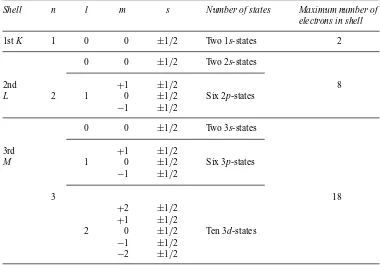
Table 1.1 Allocation of states in the first three quantum shells
Shell n l m s Number of states Maximum number of
electrons in shell
1stK 1 0 0 ±1/2 Two 1s-states 2 0 0 ±1/2 Two 2s-states
2nd +1 ±1/2 8
L 2 1 0 ±1/2 Six 2p-states
−1 ±1/2
0 0 ±1/2 Two 3s-states
3rd +1 ±1/2
M 1 0 ±1/2 Six 3p-states
−1 ±1/2
3 18
+2 ±1/2
+1 ±1/2
2 0 ±1/2 Ten 3d-states
−1 ±1/2
−2 ±1/2
When the principal quantum numbern=1,lmust be equal to zero, and an electron in this state would be designated by the symbol 1s. Such a state can only have a single value of the inner quantum numberm=0, but can have values of+12or−12for the spin quantum numbers. It follows, therefore, that there are only two electrons in any one atom which can be in a 1s-state, and that these electrons will spin in opposite directions. Thus, whenn=1, onlys-states can exist and these can be occupied by only two electrons. Once the two 1s-states have been filled, the next lowest energy state must have n=2. Herelmay take the value 0 or 1, and therefore electrons can be in either a 2s- or a 2p-state. The energy of an electron in the 2s-state is lower than in a 2p-state, and hence the 2s-states will be filled first. Once more there are only two electrons in the 2s-state, and indeed this is always true of s-states, irrespective of the value of the principal quantum number. The electrons in thep-state can have values ofm= +1, 0,−1, and electrons having each of these values formcan have two values of the spin quantum number, leading therefore to the possibility of six electrons being in any one p-state. These relationships are shown more clearly in Table 1.1.
No further electrons can be added to the state forn=2 after two 2s- and six 2p-states are filled, and the next electron must go into the state for whichn=3, which is at a higher energy. Here the possibility arises forlto have the values 0, 1 and 2 and hence, besidess- andp-states,d-states for whichl=2 can now occur. Whenl=2,mmay have the values+2,+1, 0,−1,−2 and each may be occupied by two electrons of opposite spin, leading to a total of tend-states. Finally, whenn=4, lwill have the possible values from 0 to 3, and whenl=3 the reader may verify that there are 14 4f-states.
1 2 3 4 5 6 7 8 9 10 11 12 13 14 15 16 17 18 ←New IUPAC notation IA IIA IIIA IVA VA VIA VIIA VIII IB IIB IIIB IVB VB VIB VIIB O ←Previous
IUPAC form
1H 2He
1.008 4.003
3Li 4Be 5B 6C 7N 8O 9F 10Ne
6.941 9.012 10.81 12.01 14.01 16.00 19.00 20.18
11Na 12Mg 13Al 14Si 15P 16S 17Cl 18Ar
22.99 24.31 26.98 28.09 30.97 32.45 35.45 39.95
19K 20Ca 21Sc 22Ti 23V 24Cr 25Mn 26Fe 27Co 28Ni 29Cu 30Zn 31Ga 32Ge 33As 34Se 35Br 36Kr 39.10 40.08 44.96 47.90 50.94 52.00 54.94 55.85 58.93 58.71 63.55 65.37 69.72 72.92 74.92 78.96 79.90 83.80 37Rb 38Sr 39Y 40Zr 41Nb 42Mo 43Tc 44Ru 45Rh 46Pd 47Ag 48Cd 49In 50Sn 51Sb 52Te 53I 54Xe 85.47 87.62 88.91 91.22 92.91 95.94 98.91 101.1 102.9 106.4 107.9 112.4 114.8 118.7 121.8 127.6 126.9 131.3 55Cs 56Ba 57La 72Hf 73Ta 74W 75Re 76Os 77Ir 78Pt 79Au 80Hg 81Tl 82Pb 83Bi 84Po 85At 86Rn 132.9 137.3 138.9 178.5 180.9 183.9 186.2 190.2 192.2 195.1 197.0 200.6 204.4 207.2 209.0 (210) (210) (222) 87Fr 88Ra 89Ac 104Unq 105Unp 106Unh 107Uns
(223) (226.0) (227)
←−s-block−→ ←−−−−−−−−−−−−−−−−−−−−−−−−−−d-block−−−−−−−−−−−−−−−−−−−−−−−−−−→ ←−−−−−−−−−−−−−p-block−−−−−−−−−−−−−→
Lanthanides 57La 58Ce 59Pr 60Nd 61Pm 62Sm 63Eu 64Gd 65Tb 66Dy 67Ho 68Er 69Tm 70Yb 71Lu
138.9 140.1 140.9 144.2 (147) 150.4 152.0 157.3 158.9 162.5 164.9 167.3 168.9 173.0 175.0
Actinides 89Ac 90Th 91Pa 92U 93Np 94Pu 95Am 96Cm 97Bk 98Cf 99Es 100Fm 101Md 102No 103Lr
(227) 232.0 231.0 238.0 237.0 (242) (243) (248) (247) (251) (254) (253) (256) (254) (257)
Correct (3e) (a)
Incorrect (3e) (b)
Correct (4e) (c) Figure 1.1 Application of Hund’s multiplicity rule to the electron filling of energy states.
1.3 The Periodic Table
The Periodic Table provides an invaluable classification of all chemical elements, an element being a collection of atoms of one type. A typical version is shown in Table 1.2. Of the 107 elements which appear, about 90 occur in nature; the remainder are produced in nuclear reactors or particle accelera-tors. The atomic number (Z) of each element is stated, together with its chemical symbol, and can be regarded as either the number of protons in the nucleus or the number of orbiting electrons in the atom. The elements are naturally classified into periods (horizontal rows), depending upon which electron shell is being filled, and groups (vertical columns). Elements in any one group have the electrons in their outermost shell in the same configuration and, as a direct result, have similar chemical properties. The building principle (Aufbauprinzip) for the table is based essentially upon two rules. First, the Pauli Exclusion Principle (Section 1.2.1) must be obeyed. Second, in compliance with Hund’s rule of maximum multiplicity, the ground state should always develop maximum spin. This effect is demonstrated diagrammatically in Figure 1.1. Suppose that we supply three electrons to the three ‘empty’ 2p-orbitals. They will build up a pattern of parallel spins (a) rather than paired spins (b). A fourth electron will cause pairing (c). Occasionally, irregularities occur in the ‘filling’ sequence for energy states because electrons always enter the lowest available energy state. Thus, 4s-states, being at a lower energy level, fill before the 3d-states.
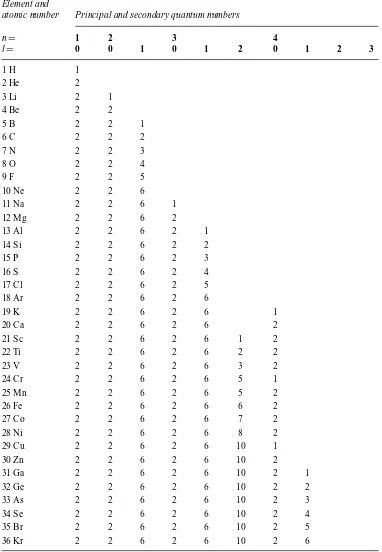
We will now examine the general process by which the Periodic Table is built up, electron by electron, in closer detail. The progressive filling of energy states can be followed in Table 1.3. The first period commences with the simple hydrogen atom, which has a single proton in the nucleus and a single orbiting electron (Z=1). The atom is therefore electrically neutral and, for the lowest energy condition, the electron will be in the 1s-state. In helium, the next element, the nucleus charge is increased by one proton and an additional electron maintains neutrality (Z=2). These two electrons fill the 1s-state and will necessarily have opposite spins. The nucleus of helium contains two neutrons as well as two protons, hence its mass is four times greater than that of hydrogen. The next atom, lithium, has a nuclear charge of three (Z=3) and, because the first shell is full, an electron must enter the 2s-state, which has a somewhat higher energy. The electron in the 2s-state, usually referred to as the valency electron, is ‘shielded’ by the inner electrons from the attracting nucleus and is therefore less strongly bonded. As a result, it is relatively easy to separate this valency electron. The ‘electron core’ which remains contains two tightly-bound electrons and, because it carries a single net positive charge, is referred to as a monovalent cation. The overall process by which electron(s) are lost or gained is known as ionization.
Table 1.3 Electron quantum numbers (Hume-Rothery, Smallman and Haworth, 1988).
Element and
atomic number Principal and secondary quantum numbers
n= 1 2 3 4
l= 0 0 1 0 1 2 0 1 2 3
1 H 1
2 He 2
3 Li 2 1
4 Be 2 2
5 B 2 2 1
6 C 2 2 2
7 N 2 2 3
8 O 2 2 4
9 F 2 2 5
10 Ne 2 2 6
11 Na 2 2 6 1
12 Mg 2 2 6 2
13 Al 2 2 6 2 1
14 Si 2 2 6 2 2
15 P 2 2 6 2 3
16 S 2 2 6 2 4
17 Cl 2 2 6 2 5
18 Ar 2 2 6 2 6
19 K 2 2 6 2 6 1
20 Ca 2 2 6 2 6 2
21 Sc 2 2 6 2 6 1 2
22 Ti 2 2 6 2 6 2 2
23 V 2 2 6 2 6 3 2
24 Cr 2 2 6 2 6 5 1
25 Mn 2 2 6 2 6 5 2
26 Fe 2 2 6 2 6 6 2
27 Co 2 2 6 2 6 7 2
28 Ni 2 2 6 2 6 8 2
29 Cu 2 2 6 2 6 10 1
30 Zn 2 2 6 2 6 10 2
31 Ga 2 2 6 2 6 10 2 1
32 Ge 2 2 6 2 6 10 2 2
33 As 2 2 6 2 6 10 2 3
34 Se 2 2 6 2 6 10 2 4
35 Br 2 2 6 2 6 10 2 5
36 Kr 2 2 6 2 6 10 2 6
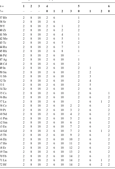
Table 1.3 (Continued)
Element and
atomic number Principal and secondary quantum numbers
n= 1 2 3 4 5 6
l= – – – 0 1 2 3 0 1 2 0
37 Rb 2 8 18 2 6 1
38 Sr 2 8 18 2 6 2
39 Y 2 8 18 2 6 1 2
40 Zr 2 8 18 2 6 2 2
41 Nb 2 8 18 2 6 4 1
42 Mo 2 8 18 2 6 5 1
43 Tc 2 8 18 2 6 5 2
44 Ru 2 8 18 2 6 7 1
45 Rh 2 8 18 2 6 8 1
46 Pd 2 8 18 2 6 10 –
47 Ag 2 8 18 2 6 10 1
48 Cd 2 8 18 2 6 10 2
49 In 2 8 18 2 6 10 2 1
50 Sn 2 8 18 2 6 10 2 2
51 Sb 2 8 18 2 6 10 2 3
52 Te 2 8 18 2 6 10 2 4
53 I 2 8 18 2 6 10 2 5
54 Xe 2 8 18 2 6 10 2 6
55 Cs 2 8 18 2 6 10 2 6 1
56 Ba 2 8 18 2 6 10 2 6 2
57 La 2 8 18 2 6 10 2 6 1 2
58 Ce 2 8 18 2 6 10 2 2 6 2
59 Pr 2 8 18 2 6 10 3 2 6 2
60 Nd 2 8 18 2 6 10 4 2 6 2
61 Pm 2 8 18 2 6 10 5 2 6 2
62 Sm 2 8 18 2 6 10 6 2 6 2
63 Eu 2 8 18 2 6 10 7 2 6 2
64 Gd 2 8 18 2 6 10 7 2 6 1 2
65 Tb 2 8 18 2 6 10 9 2 6 2
66 Dy 2 8 18 2 6 10 10 2 6 2
67 Ho 2 8 18 2 6 10 11 2 6 2
68 Er 2 8 18 2 6 10 12 2 6 2
69 Tm 2 8 18 2 6 10 13 2 6 2
70 Yb 2 8 18 2 6 10 14 2 6 2
71 Lu 2 8 18 2 6 10 14 2 6 1 2
72 Hf 2 8 18 2 6 10 14 2 6 2 2
Table 1.3 (Continued)
Element and
atomic number Principal and secondary quantum numbers
n= 1 2 3 4 5 6 7
l= – – – – 0 1 2 3 0 1 2 0
73 Ta 2 8 18 32 2 6 3 2
74 W 2 8 18 32 2 6 4 2
75 Re 2 8 18 32 2 6 5 2
76 Os 2 8 18 32 2 6 6 2
77 Ir 2 8 18 32 2 6 7 2
78 Pt 2 8 18 32 2 6 9 1
79 Au 2 8 18 32 2 6 10 1
80 Hg 2 8 18 32 2 6 10 2
81 Tl 2 8 18 32 2 6 10 2 1
82 Pb 2 8 18 32 2 6 10 2 2
83 Bi 2 8 18 32 2 6 10 2 3
84 Po 2 8 18 32 2 6 10 2 4
85 At 2 8 18 32 2 6 10 2 5
86 Rn 2 8 18 32 2 6 10 2 6
87 Fr 2 8 18 32 2 6 10 2 6 1
88 Ra 2 8 18 32 2 6 10 2 6 2
89 Ac 2 8 18 32 2 6 10 2 6 1 2
90 Th 2 18 8 32 2 6 10 2 6 2 2
91 Pa 2 18 8 32 2 6 10 2 2 6 1 2
92 U 2 18 8 32 2 6 10 3 2 6 1 2
93 Np 2 18 8 32 2 6 10 4 2 6 1 2
94 Pu 2 18 8 32 2 6 10 5 2 6 1 2
The exact electronic configurations of the later elements are not always certain but the most probable arrangements of the outer electrons are:
95 Am (5f)7(7s)2 96 Cm (5f)7(6d)1(7s)2
97 Bk (5f)8(6d)1(7s)2 98 Cf (5f)10(7s)2 99 Es (5f)11(7s)2 100 Fm (5f)12(7s)2 101 Md (5f)13(7s)2
The second short period, from sodium (Z=11) to argon (Z=18), commences with the occupation of the 3s-orbital and ends when the 3p-orbitals are full (Table 1.3). The long period which follows extends from potassium (Z=19) to krypton (Z=36) and, as mentioned previously, has the unusual feature of the 4s-state filling before the 3d-state. Thus, potassium has a similarity to sodium and lithium in that the electron of highest energy is in ans-state; as a consequence, they have very similar chemical reactivities, forming the group known as the alkali-metal elements. After calcium (Z=20), filling of the 3d-state begins.
The 4s-state is filled in calcium (Z=20) and the filling of the 3d-state becomes energetically favorable to give scandium (Z=21). This belated filling of the five 3d-orbitals from scandium to its completion in copper (Z=29) embraces the first series of transition elements. One member of this series, chromium (Z=24), obviously behaves in an unusual manner. Applying Hund’s rule, we can reason that maximization of parallel spin is achieved by locating six electrons, of like spin, so that five fill the 3d-states and one enters the 4s-state. This mode of fully occupying the 3d-states reduces the energy of the electrons in this shell considerably. Again, in copper (Z=29), the last member of this transition series, complete filling of all 3d-orbitals also produces a significant reduction in energy. It follows from these explanations that the 3d- and 4s-levels of energy are very close together. After copper, the energy states fill in a straightforward manner and the first long period finishes with krypton (Z=36). It will be noted that lanthanides (Z=57–71) and actinides (Z=89–103), because of their state-filling sequences, have been separated from the main body of Table 1.2. Having demonstrated the manner in which quantum rules are applied to the construction of the Periodic Table for the first 36 elements, we can now examine some general aspects of the classification.
When one considers the small step difference of one electron between adjacent elements in the Periodic Table, it is not really surprising to find that the distinction between metallic and non-metallic elements is imprecise. In fact, there is an intermediate range of elements, the metalloids, which share the properties of both metals and non-metals. However, we can regard the elements which can readily lose an electron, by ionization or bond formation, as strongly metallic in character (e.g. alkali metals). Conversely, elements which have a strong tendency to acquire an electron and thereby form a stable configuration of two or eight electrons in the outermost shell are non-metallic (e.g. the halogens fluorine, chlorine, bromine, iodine). Thus, electropositive metallic elements and the electronegative non-metallic elements lie on the left- and right-hand sides of the Periodic Table, respectively. As will be seen later, these and other aspects of the behavior of the outermost (valence) electrons have a profound and determining effect upon bonding, and therefore upon electrical, magnetic and optical properties. Prior to the realization that the frequently observed periodicities of chemical behavior could be expressed in terms of electronic configurations, emphasis was placed upon ‘atomic weight’. This quantity, which is now referred to as relative atomic mass, increases steadily throughout the Periodic Table as protons and neutrons are added to the nuclei. Atomic mass2determines physical properties such as density, specific heat capacity and ability to absorb electromagnetic radiation: it is therefore very relevant to engineering practice. For instance, many ceramics are based upon the light elements aluminum, silicon and oxygen, and consequently have a low density, i.e.<3000 kg m−3.
1.4 Interatomic bonding in materials
Matter can exist in three states and, as atoms change directly from either the gaseous state (desublima-tion) or the liquid state (solidifica(desublima-tion) to the usually denser solid state, the atoms form aggregates in three-dimensional space. Bonding forces develop as atoms are brought into proximity to each other. Generally, there is an attractive force between the atoms but at close range a repulsive force exists.
Crystal spacing
Attraction Repulsion
0 ⫹
⫺
Potential energy
r0
Er
0
Increasing interatomic distance r
Figure 1.2 Variation in potential energy with interatomic distance.
The equilibrium spacing is given when these two forces balance. The energy of interaction decreases as the atoms approach and has its lowest value at the equilibrium spacing, as shown in Figure 1.2. The potential energyUof a pair of atoms can be written as:
U = −A rm+
B
rn (1.1)
whereris the atom separation withm<n, and the first term is attractive, the second repulsive. At r<ro, the equilibrium value, the repulsive force dominates andU rises. The forceFis given by the
rate of change of energy with distance dU/drand is zero atr=ro.
The nature of the bonding forces has a direct effect upon the type of solid structure which develops and therefore upon the physical properties of the material. Melting point provides a useful indication of the amount of thermal energy needed to sever these interatomic (or interionic) bonds. Thus, some solids melt at relatively low temperatures (m.p. of tin=232◦C), whereas many ceramics melt at extremely high temperatures (m.p. of alumina exceeds 2000◦C). It is immediately apparent that bond strength has far-reaching implications in all fields of engineering.
Customarily we identify four principal types of bonding in materials, namely metallic bonding, ionic bonding, covalent bonding and the comparatively much weaker van der Waals bonding. However, in many solid materials it is possible for bonding to be mixed, or even intermediate, in character. We will first consider the general chemical features of each type of bonding; in later sections we will examine the resultant disposition of the assembled atoms (ions) in three-dimensional space.
⫹
⫹
⫹
⫹
⫹
⫹
⫺ ⫹ ⫺
⫹
⫹ ⫺
⫹ ⫺
⫹
⫺ ⫹
⫺ ⫹
⫺ ⫹
⫺
⫹ ⫺ (a) Sodium (Z ⫽ 11)
(c) Carbon (Z ⫽ 6) (d) Polarized atoms (b) Magnesium (Z ⫽ 12)
and oxygen (Z ⫽ 8)
Figure 1.3 Schematic representation of: (a) metallic bonding, (b) ionic bonding, (c) covalent bonding and (d) van der Waals bonding.
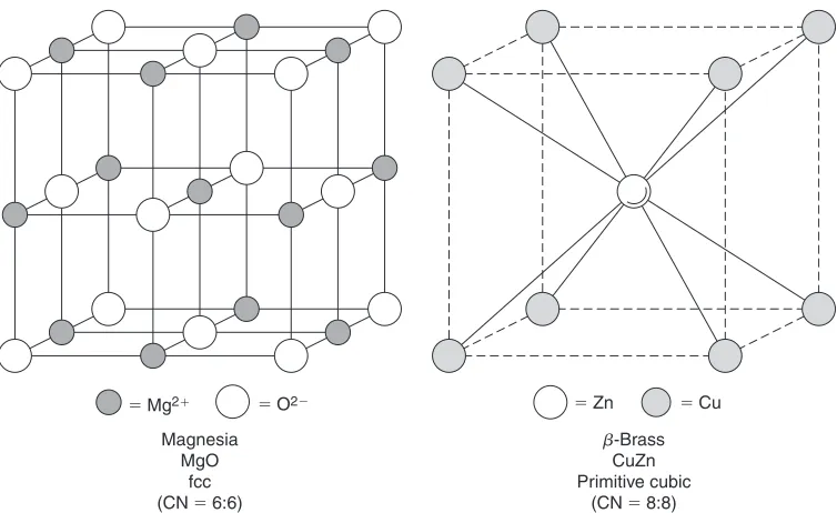
closed shell. For example, the ionic structure of magnesia (MgO), a ceramic oxide, forms when each magnesium atom (Z=12) loses two electrons from its M-shell (n=3) and these electrons are acquired by an oxygen atom (Z=8), producing a stable octet configuration in its L-shell (Table 1.3). Overall, the ionic charges balance and the structure is electrically neutral (Figure 1.3b). Anions are usually larger than cations. Ionic bonding is omnidirectional, essentially electrostatic in character and can be extremely strong; for instance, magnesia is a very useful refractory oxide (m.p.=2930◦C). At low to moderate temperatures, such structures are electrical insulators but, typically, become conductive at high temperatures when thermal agitation of the ions increases their mobility.
Sharing of valence electrons is the key feature of the third type of strong primary bonding. Cova-lent bonds form when valence electrons of opposite spin from adjacent atoms are able to pair within overlapping spatially directed orbitals, thereby enabling each atom to attain a stable electronic configuration (Figure 1.3c). Being oriented in three-dimensional space, these localized bonds are unlike metallic and ionic bonds. Furthermore, the electrons participating in the bonds are tightly bound so that covalent solids, in general, have low electrical conductivity and act as insulators, some-times as semiconductors (e.g. silicon). Carbon in the form of diamond is an interesting prototype for covalent bonding. Its high hardness, low coefficient of thermal expansion and very high melting point (3300◦C) bear witness to the inherent strength of the covalent bond. First, using the (8−N) Rule, in which N is the Group Number3in the Periodic Table, we deduce that carbon (Z=6) is tetravalent; that
is, four bond-forming electrons are available from the L-shell (n=2). In accordance with Hund’s Rule (Figure 1.1), one of the two electrons in the 2s-state is promoted to a higher 2p-state to give a maximum spin condition, producing an overall configuration of 1s22s12p3in the carbon atom. The outermost second shell accordingly has four valency electrons of like spin available for pairing. Thus, each carbon atom can establish electron-sharing orbitals with four neighbors. For a given atom, these four bonds are of equal strength and are set at equal angles (109.5◦) to each other and therefore exhibit tetrahedral symmetry. (The structural consequences of this important feature will be discussed in Section 1.9.2.) This process by whichs-orbitals andp-orbitals combine to form projecting hybridsp-orbitals is known as hybridization. It is observed in elements other than carbon. For instance, trivalent boron (Z=5) forms three co-planarsp2-orbitals. In general, a large degree of overlap ofsp-orbitals and/or a high electron density within the overlap ‘cloud’ will lead to an increase in the strength of the covalent bond. As indicated earlier, it is possible for a material to possess more than one type of bonding. For example, in calcium silicate (Ca2SiO4), calcium cations Ca2+are ionically bonded to tetrahedral
SiO44−clusters in which each silicon atom is covalently bonded to four oxygen neighbors.
The final type of bonding is attributed to the van der Waals forces which develop when adjacent atoms, or groups of atoms, act as electric dipoles. Suppose that two atoms which differ greatly in size combine to form a molecule as a result of covalent bonding. The resultant electron ‘cloud’ for the whole molecule can be pictured as pear-shaped and will have an asymmetrical distribution of electron charge. An electric dipole has formed and it follows that weak directed forces of electrostatic attraction can exist in an aggregate of such molecules (Figure 1.3d). There are no ‘free’ electrons, hence electrical conduction is not favored. Although secondary bonding by van der Waals forces is weak in comparison to the three forms of primary bonding, it has practical significance. For instance, in the technologically important mineral talc, which is hydrated magnesium silicate Mg3Si4O10(OH)2,
the parallel, covalently bonded layers of atoms are attracted to each other by van der Waals forces. These layers can easily be slid past each other, giving the mineral its characteristically slippery feel. In thermoplastic polymers, van der Waals forces of attraction exist between the extended covalently bonded hydrocarbon chains; a combination of heat and applied shear stress will overcome these forces and cause the molecular chains to glide past each other. To quote a more general case, molecules of water vapor in the atmosphere each have an electric dipole and will accordingly tend to be adsorbed if they strike solid surfaces possessing attractive van der Waals forces (e.g. silica gel).
Worked example
The potential energyUof a pair of atoms in a solid is given by equation (1.1).
(i) Outline the physical significance of the two terms and indicate the values of the two constants mandn.
(ii) Taking the value ofm=2 and n=10, calculate the values of AandBfor a stable atomic configuration wherer=3×10⁻¹⁰m andU= −4 eV. Calculate the force required to break the diatomic configuration.
Solution
(i) −A/rmis an attractive potential related to the type of bonding in the crystal.B/rnis a repulsive potential when the ions get close. The value ofm<n, typicallyn∼12 for ionic solids. (ii) The energy function now reads:
U = −A r2 +
At equilibrium atr=ro,
Thus, maximum force to break bond:
F=ddU
Energy
Higher level unoccupied in the free atom
Valency level Crystal
spacing
Decreasing interatomic spacing
Levels of core electrons
Figure 1.4 Broadening of atomic energy levels in a metal.
(a)
Emax E
N(E)
Energy
(b)
Emax
Ener
g
y
Figure 1.5 (a) Density of energy levels plotted against energy. (b) Filling of energy levels by electrons at absolute zero. At ordinary temperatures some of the electrons are thermally excited to higher levels than that corresponding toEmax, as shown by the broken curve in (a).
maximum of 2Nelectrons. Clearly, in the lowest energy state of the metal all the lower energy levels are occupied.
The energy gap between successive levels is not constant but decreases as the energy of the levels increases. This is usually expressed in terms of the density of electronic statesN(E) as a function of the energyE. The quantityN(E)dEgives the number of energy levels in a small energy interval dE, and for free electrons is a parabolic function of the energy, as shown in Figure 1.5.