Optimal Scheduling of Refinery Crude Oil Operations

(1)

Carnegie Mellon University

Research Showcase

Dissertations

Theses and Dissertations

12-1-2010

Optimal Scheduling of Refinery Crude-Oil

Operations

Sylvain Mouret

Carnegie Mellon University

Follow this and additional works at:

http://repository.cmu.edu/dissertations

This is brought to you for free and open access by the Theses and Dissertations at Research Showcase. It has been accepted for inclusion in Dissertations by an authorized administrator of Research Showcase. For more information, please contactresearch-showcase@andrew.cmu.edu.

Recommended Citation

(2)

Optimal Scheduling of Refinery

Crude-Oil Operations

A DISSERTATION

Submitted to the Graduate School in Partial Fulfillment of the Requirements

for the degree of

Doctor of Philosophy

in

Chemical Engineering

by

Sylvain Mouret

Carnegie Mellon University

(3)

Acknowledgments

First of all, I would like to express my most sincere gratitude to my advisor Professor Ignacio

E. Grossmann for his inestimable guidance and support over the course of my Ph.D. He has

managed to create a productive yet friendly environment and proved to be an abundant

source of knowledge for myself. I cannot thank him enough for his confidence in me and his

deep implication in my studies and in my life.

Besides my advisor, I would like to thank my thesis committee members – Professors

Lorenz Biegler, Nikolaos Sahinidis, John Hooker, and Willem-Jan van Hoeve for their time

and valuable comments.

I would like to thank Pierre Pestiaux, my supervisor at Total, whose strong commitment

to the project and never-ending enthusiasm has made this thesis possible.

I would also like to thank Philippe Bonnelle for bringing his experience and his insightful

suggestions into the project as well as other collaborators at SOG and CReG, for their useful

feedback on my work and friendly support. Furthermore, I am grateful to Total Refining &

Marketing for financial support of this project.

I wish to express my thankfulness for all my past and present workmates in the PSE group

for setting a productive mood in the office and a diverting atmosphere out of work. Among

them I would like to specifically mention Rosanna Franco, Gonzalo Guill´en Gos´albez,

Ri-cardo Lima, Rodrigo L´opez-Negrete de la Fuente, Mariano Martin, Roger Rocha, Sebastian

Terrazas, and Victor Zavala with whom I share many unforgettable memories.

I would also like to thank my fellow football and tennis teammates, Tarot card players,

French speaking lunchers, barbecue grillers, etc... who made my Pittsburgh experience a

very enjoyable one.

I want to express my gratitude to my family who has always been there when I needed

(4)

Last but not least, I cannot thank enough my beloved fianc´ee Charlotte for her patience

and for standing by me during the past three and a half years. Her unconditional love is

(5)

Abstract

This thesis deals with the development of mathematical models and algorithms for

optimiz-ing refinery crude-oil operations schedules. The problem can be posed as a mixed-integer

nonlinear program (MINLP), thus combining two major challenges of operations research:

combinatorial search and global optimization.

First, we propose a unified modeling approach for scheduling problems that aims at

bridging the gaps between four different time representations using the general concept of

priority-slots. For each time representation, an MILP formulation is derived and

strength-ened using the maximal cliques and bicliques of the non-overlapping graph. Additionally,

we present three solution methods to obtain global optimal or near-optimal solutions. The

scheduling approach is applied to single-stage and multi-stage batch scheduling problems

as well as a crude-oil operations scheduling problem maximizing the gross margin of the

distilled crude-oils.

In order to solve the crude-oil scheduling MINLP, we introduce a two-step MILP-NLP

procedure. The solution approach benefits from a very tight upper bound provided by the

first stage MILP while the second stage NLP is used to obtain a feasible solution.

Next, we detail the application of the single-operation sequencing time representation

to the crude-oil operations scheduling problem. As this time representation displays many

symmetric solutions, we introduce a symmetry-breaking sequencing rule expressed as a

deterministic finite automaton in order to efficiently restrict the set of feasible solutions.

Furthermore, we propose to integrate constraint programming (CP) techniques to the

branch & cut search to dynamically improve the linear relaxation of a crude-oil operations

scheduling problem minimizing the total logistics costs expressed as a bilinear objective.

CP is used to derived tight McCormick convex envelopes for each node subproblem thus

(6)

Finally, the refinery planning and crude-oil scheduling problems are simultaneously solved

using a Lagrangian decomposition procedure based on dualizing the constraint linking crude

distillation feedstocks in each subproblem. A new hybrid dual problem is proposed to update

the Lagrange multipliers, while a simple heuristic strategy is presented in order to obtain

feasible solutions to the full-space MINLP. The approach is successfully applied to a small

(7)

List of Tables

1.1 Optimization techniques used in different MINLP solvers. . . 12

2.1 Resource requirements for case study. . . 22

2.2 Time representations nomenclature. . . 27

2.3 Data for single-stage batch scheduling problems. . . 43

2.4 Unit cardinality bounds depending on parametern for SSBSP29. . . 46

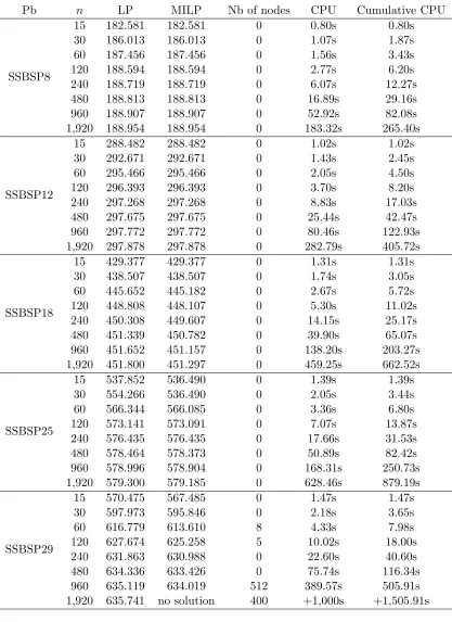
2.5 MOS computational results for single-stage batch scheduling problems. . . . 49

2.6 MOS-SST computational results for single-stage batch scheduling problems. 52 2.7 MOS-FST computational results for single-stage batch scheduling problems. 54 2.8 Data for multi-stage batch scheduling problems. . . 58

2.9 MOS computational results for multi-stage batch scheduling problems. . . . 61

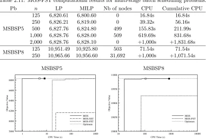
2.10 MOS-SST computational results for multi-stage batch scheduling problems. 63 2.11 MOS-FST computational results for multi-stage batch scheduling problems. 65 3.1 Data for COSP1. . . 71

3.2 MOS computational results for crude-oil scheduling problems. . . 87

3.3 MOS-SST computational results for crude-oil scheduling problems. . . 88

3.4 MOS-FST computational results for crude-oil scheduling problems. . . 89

3.5 Performance of different MINLP algorithms for crude-oil scheduling problems. 90 4.1 Maximal cliques and bicliques for COSP2 and COSP3. . . 93

4.2 Cliques and bicliques selections a,b, and c for COSP2 and COSP3. . . 94

4.3 List of sequences belonging to regular language L7. . . 98

4.4 SOS computational results for crude-oil operations scheduling problems. . . 101

4.5 Size and performance of Basic and Extended models on COSP1 (13 slots). . 106

4.6 Size of MOS, MOS-SST, MOS-FST, and SOS models for crude-oil scheduling problems. . . 108

5.1 Cost data for crude-oil operations scheduling problems. . . 113

5.2 Results obtained with BasicRelaxation and ExtendedRelaxation algorithms. 118 5.3 Results obtained with diferrent MINLP algorithms on COSP1 and COSP2. 119 6.1 Crude-oil scheduling data for case study. . . 126

6.2 Lagrangian iterations statistics (6 priority-slots, NLP=SNOPT). . . 142

6.3 Lagrangian iterations statistics (7 priority-slots, NLP=SNOPT). . . 143

6.4 Comparative performance of different MINLP algorithms. . . 146

6.5 Crude cut prices and specification for larger refinery problem. . . 150

(12)

6.7 Lagrangian iterations statistics for larger refinery problem (6 priority-slots,

NLP=CONOPT). . . 152

6.8 Optimal Lagrange multipliers for each crude and each CDU mode. . . 153

6.9 Comparative performance of several MINLP algorithms for larger refinery problem (NLP solver: CONOPT). . . 153

6.10 Blend compositions in the optimal solution of larger refinery problem. . . . 154

B.1 Data for COSP1. . . 181

(13)

List of Figures

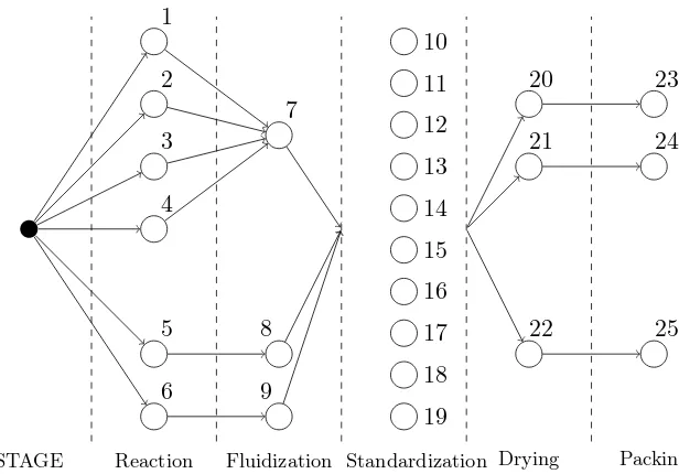
1.1 A typical multi-stage batch process from Pinto and Grossmann (1995). . . . 3

1.2 A typical oil refining process from M´endez et al. (2006b). . . 6

1.3 Schematic flow diagram of a typical oil refinery from Wikipedia (2010). . . 7

1.4 Crude-oil scheduling problem 1 from Lee et al. (1996). . . 9

2.1 Four steps optimization approach. . . 20

2.2 Non-overlapping matrix and graph for case study. . . 23

2.3 A unique schedule obtained through different time representations. . . 24

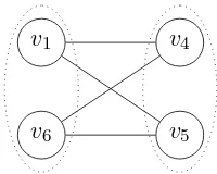
2.4 Biclique ({v1, v6};{v4, v5}). . . 34

2.5 Assignment constraint using consecutive time-points. . . 37

2.6 Non-overlapping graph with isolated cliques for SSBSP8. . . 44

2.7 Effect of the minimum priority-slot usage constraint. . . 50

2.8 Equivalent MOS and SOS assignments for SSBSP12. . . 55

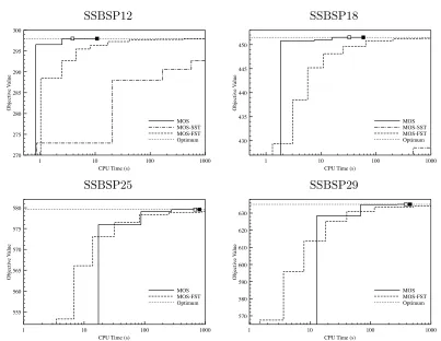
2.9 Comparison of time representations for single-stage batch scheduling problems. 56 2.10 Partial non-overlapping graph with isolated cliques for MSBSP5. . . 59

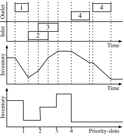
2.11 Comparison of time representations for multi-stage batch scheduling problems. 65 3.1 Example of tank schedule. . . 70

3.2 Sub-optimal schedule for COSP1 (profit: $6,925,000). . . 72

3.3 Optimal schedule for COSP1 (profit: $7,975,000). . . 73

3.4 Refinery crude-oil scheduling system for problem COSP2 and COSP3. . . . 79

3.5 Non-overlapping graph for crude-oil examples 2 and 3. . . 80

3.6 Two step decomposition strategy. . . 81

3.7 Optimal schedule for COSP2 (profit: $10,117,000). . . 83

3.8 Schedule obtained for COSP3 within 2.3% optimality gap (profit: $8,540,000). 84 3.9 Optimal schedule for COSP2 with late vessel arrivals (profit: $9,775,000). . 85

3.10 Optimal schedule for COSP2 with late vessel arrivals and fixed initial deci-sions (profit: $9,609,000). . . 86

4.1 Symmetric sequences of operations for COSP1. . . 96

4.2 Automaton DFA7 recognizing regular languageL7. . . 98

4.3 Automaton recognizing the regular languageL. . . 99

4.4 Performance of the SOS model on crude-oil scheduling problems (MILP solver: Xpress). . . 104

4.5 Performance of the Basic and Extended models on COSP1 (6 to 13 slots). . 106

4.6 Comparison of time representations for crude-oil scheduling problems. . . . 107

(14)

6.1 Basic refinery planning system. . . 122

6.2 Refinery planning case study. . . 124

6.3 Refinery crude-oil scheduling system for COSP1. . . 125

6.4 Economic interpretation of the Lagrangian decomposition. . . 130

6.5 General iterative primal-dual algorithm. . . 132

6.6 Plots of the feasible space of ( ˆP_DK+1). . . 133

6.7 Iterative primal-dual algorithm with heuristic step. . . 135

6.8 Crude-oil scheduling and multi-period refinery planning integration. . . 137

6.9 Disaggregated CDU feedstocks synchronization. . . 138

6.10 Complete algorithm implementation. . . 141

6.11 Lagrangian iteration objective values (6 priority-slots, NLP=SNOPT). . . . 144

6.12 Lagrangian iteration objective values (7 priority-slots, NLP=SNOPT). . . . 144

6.13 Lagrange multiplier updates (6 priority-slots, NLP=SNOPT). . . 145

6.14 Lagrange multiplier updates (7 priority-slots, NLP=SNOPT). . . 145

6.15 Blend compositions in solutions obtained with 6 priority-slots. . . 147

6.16 Planning model for larger refinery problem. . . 149

6.17 Refinery crude-oil scheduling system for COSP3. . . 150

6.18 Lagrangian iteration objective values for larger refinery problem (6 priority-slots, NLP=CONOPT). . . 152

B.1 Refinery crude-oil scheduling system for COSP1. . . 181

B.2 Refinery crude-oil scheduling system for COSP2 and COSP3. . . 182

B.3 Refinery crude-oil scheduling system for COSP4. . . 183

(15)

Chapter 1 Introduction

Optimization in the oil refining industry began with the use of linear programming (LP) to

perform process and economic analysis of industrial plants (see Garvin et al., 1957; Manne,

1958). Many refinery problems are now addressed with algorithms based on mathematical

models: refinery planning, crude-oil operations scheduling, final product blending, crude-oil

transportation, final product shipping, and profitability improvement plans (for instance,

see Pinto et al., 2000). In general, problem-specific techniques are used to solve each model

independently from the others. The goal of this thesis is to develop a general methodology

towards enterprise-wide optimization of oil refineries (Grossmann, 2005). Due to the

struc-tural diversity of the problems to be solved, the challenge is to effectively integrate different

optimization techniques in order to generate near-optimal enterprise-wide solutions. The

industrial applications addressed in this thesis are related to single-stage and multi-stage

batch processes, medium-term planning of refining operations and short-term scheduling of

crude-oil operations. The objectives of the thesis are as follows:

1. Develop a unified modeling approach for solving process scheduling problems

2. Apply the proposed time representations to schedule and optimize batch processes

and crude-oil operations

3. Develop and implement general solution methods to effectively solve such problems

and obtain near-optimal solutions with rigorous optimality estimates

4. Develop a method for integrating mixed-integer linear programming and constraint

programming for improving the linear relaxation of mixed-integer nonlinear programs

5. Apply advanced Lagrangian decomposition techniques to simultaneously solve refinery

(16)

1.1 Single-Stage and Multi-Stage Batch Scheduling

In this chapter, an overview of single-stage and multi-stage batch scheduling problems

is presented followed by a description of the refinery planning and crude-oil scheduling

problems. The different optimization techniques used are then reviewed and we conclude

with an overview of the chapters in the thesis.

1.1 Single-Stage and Multi-Stage Batch Scheduling

The chemical industry has been marked by an increase of product diversification, which

in turn has led to an increase in the complexity of operations of plant facilities. Chemical

companies are now facing the challenge of meeting global demands of multiple products

while increasing plant capacities to achieve economies of scale (Wassick, 2009). Operating

optimally such plants can be non-trivial as decision-makers have to account for demand

deadlines, process constraints, and limited resources. Therefore, the scheduling of chemical

processes has received much attention over the past 20 years. Two major categories of

processes have been outlined and addressed: sequential and network-based processes (see

process classification in M´endez et al., 2006a). The main difference lies in the fact that

network processes may display recycle loops which sequential processes do not.

Recently, several research groups have reviewed the different trends in process scheduling

for general purpose plants. Floudas and Lin (2004) provided an extensive comparison

of discrete-time and continuous-time formulations. In M´endez et al. (2006a), a complete

classification of scheduling approaches is presented in addition to the process classification.

In this thesis, we study single-stage and multi-stage batch scheduling problems. Figure 1.1

depicts a typical multi-stage batch process. A finite number of batches with fixed sizes have

to be processed going through a given set of successive stages. In each stage, a finite set of

parallel units is available. The processing times for each batch and each stage may be

unit-dependent. Stages with limited resources or high processing times are often calledbottleneck

stages. Different policies can be used for interstage storage: unlimited intermediate storage

(17)

STAGE Reaction Fluidization Standardization Drying Packing

Figure 1.1: A typical multi-stage batch process from Pinto and Grossmann (1995).

Two main scheduling approaches have been developed to solve batch scheduling problems:

precedence-based and slot-based models.

The idea of using disjunctive programming principles (see Balas, 1985) to solve chemical

process scheduling problems was initially introduced by Cerd´a et al. (1997) who proposed a

mathematical model for scheduling single-stage multiproduct batch plants. Among others,

Gupta and Karimi (2003); Méndez and Cerdá (2007); Marchetti and Cerdá (2009) have

successively improved and extended precedence-based formulations and applied them to

multistage batch scheduling problems. They consider complex scheduling features such as

sequence-dependent changeovers, unit release times, or discrete resource constraints. The

basic idea is to use binary variables to represent the precedence relations between each pair

of operations. The corresponding models usually involve many big-M constraints, which

may result in poor LP relaxations. However, these formulations lead to models of modest

size which often makes them tractable. In principle, these formulations can be used to

represent any type of scheduling constraints, but global features such as limited inventory

(18)

and often require additional big-M constraints.

Another scheduling approach consists of using the concept of slots in order to assign

a position for each operation in a sequence. Depending on the formulation used, these

positions are directly or indirectly linked to the timing decisions. These types of formulations

are particularly efficient to represent global scheduling features as its inherent sequencing

representation may involve as many operations as needed.

Ku and Karimi (1988) presented an MILP formulation for multi-stage batch scheduling

problem with finite interstage storage and exactly one unit per stage. Two heuristics are

presented in order to solve the problem faster and compared to the optimal MILP approach.

Pinto and Grossmann (1995) developed a continuous-time slot-based mathematical

for-mulation and considered a batch preordering heuristic to improve the computational

re-quirements. This approach was applied to several examples with unit-dependent processing

times and changeovers.

Hui et al. (2000) addressed the issue of sequence-dependent changeovers using a

simi-lar slot-based MILP model. Later, Gupta and Karimi (2003) improved the mathematical

formulation using fewer variables and constraints to reduce the computational times.

Castro and Grossmann (2005) used the resource-task network representation (RTN) to

model multi-stage batch scheduling problem. They developed and implemented several

scheduling approaches and presented extensive computational results.

Recently, Prasad and Maravelias (2008) solved the integrated batching and scheduling

problem. It consists of simultaneously making the following decisions: batch selection and

sizing, unit assignment and sequencing of batches on each unit.

Finally, it should be noted that models for structures others than multi-stage batch plants

have also been extensively studied using representations as the state-task network (Kondili

(19)

1.2 Optimization of Oil Refineries

Oil refineries are a key element in the valorization of crude-oils into energy. They consist of

highly flexible plants that can refine crude-oils produced from many locations in the world,

with very different properties, into useful petroleum products: LPG, gasoline and diesel

fuels, kerosene, heating oil, bitumen, etc.

As depicted in Figure 1.2, the refining process can be decomposed into 3 main phases:

crude-oil unloading and preparation for distillation, fractionation and reaction operations,

final product blending and shipping. Based on this spatial decomposition, the following

off-line optimization problems have been addressed in the literature:

1. Refinery planning (see section 1.2.1)

2. Crude-oil operations scheduling (see section 1.2.2)

3. Final product blending operations scheduling with recipe optimization (see M´endez

et al., 2006b)

4. Scheduling of internal refinery product-specific subsystems:

- for LPG, see Pinto and Moro (2000)

- for fuel oils and asphalts, see Joly and Pinto (2003)

- for lube oils and paraffins, see Casas-Liza and Pinto (2005)

Given the diversity and the complexity of the subsystems to be studied, this thesis is focused

on the integration of the first two refinery optimization problems.

1.2.1 Refinery Planning

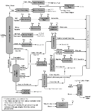
Refinery operators typically determine their annual and monthly plan by solving the refinery

planning problem. It is based on a steady-state flowsheet optimization of a plant with

multiple heterogenous units (see Fig. 1.3). The objective is to maximize the plant’s net

present value determined by sales revenues minus purchase and operating costs. In addition

to process constraints, the problem also considers crude availabilities as well as product

(20)

Figure 1.2: A typical oil refining process from M´endez et al. (2006b).

The refinery planning problem was one of the first industrial applications of linear

pro-gramming (Bodington and Baker, 1990). However, the solution methods have evolved

towards successive linear programming (SLP) in order to better account for the nonlinear

nature of the refining process. In particular, the nonlinearities in the refinery model arise

from pooling equations and advanced process models.

The pooling problem has received much attention in the literature since the 70’s. It

usu-ally consists of optimizing feedstocks purchases, product blending operations and product

sales while taking into account product availabilities, product demands, property

specifi-cations, and pool capacities. Haverly (1978); Hart (1978); Haverly (1980) developed and

experimented the distributive recursion approach, a technique proved to be equivalent to

classical SLP (see Lasdon and Joffe, 1990) in order to solve it.

Several authors have successively addressed the issue of global optimization of pure

pool-ing problems. The techniques used range from generalized Benders decomposition (Floudas

and Aggarwal, 1990), Lagrangian relaxation (Floudas and Visweswaran, 1993; Adhya et al.,

1999), or spatial Branch and Bound (Foulds et al., 1992; Quesada and Grossmann, 1995a;

Audet et al., 2000) to reformulation-linearization techniques (Audet et al., 2000; Meyer and

(21)

Figure 1.3: Schematic flow diagram of a typical oil refinery from Wikipedia (2010).

2009). Extensive reviews of pooling formulations and solution methods can be found in

Audet et al. (2004); Misener and Floudas (2009).

Some examples of nonlinear refinery planning problems including pooling constraints

and nonlinear process models can be found in Pinto and Moro (2000); Li et al. (2005);

Alhajri et al. (2008). Although commercial solvers such as GRTMPS (Haverly Systems),

PIMS (Aspen Tech), and RPMS (Honeywell Hi-Spec Solutions) implement successive linear

(22)

solvers can also be used, although they may not guarantee global optimality of the solution.

A major issue with refinery planning is that most models are single-period models in

which the refinery is assumed to operate in the same state over the whole planning period

(typically 1 month). Therefore, the planning solution is used as a tactical goal for refinery

operators rather than as an operational tool. In particular, crude distillation unit (CDU)

feedstock decisions returned by the refinery planning problem are usually not applicable in

the field due to crude logistics constraints. These are described in the crude-oil operations

scheduling problem.

1.2.2 Crude-Oil Operations Scheduling

The optimal scheduling of crude-oil operations have been studied since the 90’s and has

been shown to lead to multimillion dollar benefits by Kelly and Mann (2003) as it is the

first stage of the oil refining process. It involves crude-oil unloading from crude marine

vessels (at berths or jetties), or from a pipeline to storage tanks, transfers from storage

tanks to charging tanks and atmospheric distillations of crude-oil mixtures from charging

tanks (see Fig. 1.4). The crude is then processed in order to produce basic products which

are then blended into finished products (see section 1.2.1). In this thesis, we assume that

the schedule of the crude supply is given. The production demands are determined by

the long-term refinery planning, either sequentially (chapters 3, 4 and 5) or simultaneously

(chapter 6). The following objectives are considered:

1. Maximization of crude gross margins (chapters 3 and 4)

2. Minimization of total logistics costs (chapter 5)

3. Maximization of total refinery profit as expressed in the planning problem (chapter 6)

Shah (1996) proposed to use mathematical programming techniques to find crude-oil

schedules exploiting opportunities to increase economic benefits. Lee et al. (1996)

con-sidered a crude-oil scheduling problem involving crude unloading at berths, and

(23)

1.3 Mixed-Integer Optimization Tools

Crude Vessels

Storage Tanks Charging Tanks

CDU

1

2

3

4

5

6

7

8

Figure 1.4: Crude-oil scheduling problem 1 from Lee et al. (1996).

Wenkay et al. (2002) improved the model and proposed an iterative approach to solve the

MINLP model, taking into account the nonlinear blending constraints.

Pinto et al. (2000), Moro and Pinto (2004), and Reddy et al. (2004) used a global event

formulation to model refinery systems involving crude-oil unloading from pipeline or jetties.

The scheduling horizon is divided into fixed length sub-intervals, which are then divided in

several variable length time-slots.

In parallel, Jia et al. (2003) developed an operation specific event model and applied it

to the problems introduced by Lee et al. (1996) using a linear approximation of storage

costs. A comparison of computational performance between both continuous-time and

discrete-time models was given showing significant decreases in CPU time for the former

model. Also, solutions that are not guaranteed to be globally optimal were obtained using

standard MINLP algorithms.

Recently, Furman et al. (2007) presented a more accurate version of the event-point

formulation, and Karuppiah et al. (2008) later addressed the global optimization of this

model using an outer-approximation algorithm where the MILP master problem is solved

by adding cuts from a Lagrangian decomposition. While rigorous, this method can be

computationally expensive.

1.3 Mixed-Integer Optimization Tools

Scheduling problems are among the most challenging optimization problems, both in terms

(24)

see Kallrath, 2002), constraint programming (CP, see Baptiste et al., 2001) and genetic

algorithm (GA, see Mitchell, 1998) techniques have been used to tackle these problems.

CP has proved to be very efficient for solving scheduling problems but it is rarely used to

solve problems arising in the chemical engineering field. One of the reason is that CP is

very efficient at sequencing tasks or jobs that are defined a priori (e.g. job-shop problems

in discrete manufacturing). However, the scheduling of chemical processes usually involves

both defining and sequencing the tasks that should be performed. Defining tasks means

choosing a batch size or a unit operating mode for example. As a consequence, LP based

techniques have been preferred with formulations essentially based on time grids as it easily

allows modeling tank or unit capacity at the end of each time interval (see Floudas and Lin,

2004; M´endez et al., 2006b).

In this thesis, we aim at solving optimization problems involving both continuous and

discrete decisions. Many computational techniques have emerged from the area of

mixed-integer optimization in order to solve problems with different characteristics (linear,

non-linear, convex, non-convex, purely integer, ...), including :

1. mixed-integer linear programming (MILP)

2. mixed-integer nonlinear programming (MINLP)

3. constraint programming (CP)

4. Lagrangian relaxation

In this section, we present brief reviews of these four optimization techniques as well as

symmetry-breaking approaches.

1.3.1 Mixed-Integer Linear Programming

Mixed-integer linear programming is used to model many decision problems from industry

(for example, process scheduling, production planning, resource allocation and supply chain

management). However, solving such combinatorial models is NP-hard (see Nemhauser and

(25)

to solve these problems in reasonable times. Two main techniques have emerged:

branch-and-bound (Land and Doig, 1960) and cutting planes (Gomory, 1958). Both are based on

theLP relaxation of the MILP. This relaxation is obtained by considering integer variables

as continuous variables with identical bounds: it can also be called continuous relaxation

orpolytope relaxation.

The branch-and-bound technique consists of searching through a tree defined by

succes-sive assignments of integer values to integer variables. At each node of this tree, an LP is

solved in order to obtain a local node optimality bound (e.g. upper bound for

maximiza-tion problems); the global optimality bound is the best bound among all open nodes (i.e.

unprocessed nodes). If the solution of this LP is integral, it provides a global feasibility

bound (e.g. lower bound for maximization problems). The search continues until all nodes

have been processed (0% optimality gap) or until the optimality gap is below a specified

tolerance.

The cutting plane algorithm consists of iteratively solving the LP relaxation and

gen-erating additional constraints (called cutting planes or cuts) that cut off the current LP

solution. The procedure is stopped when the LP solution is integral. Although this can be

achieved in a finite number of steps, in practice a large number of iterations are required.

The branch-and-cut procedure is a combination of the two aforementioned techniques.

The cutting plane algorithm is used to tighten the LP relaxation at each node, thus

im-proving the optimality bound (local and potentially global too). Branching occurs whenever

the optimality bound cannot be significantly improved.

Recent reviews of MILP techniques can be found in Bixby et al. (1999); Johnson et al.

(2000). The best known MILP solvers (CPLEX, Xpress, and Gurobi) all implement the

branch-and-cut procedure and are widely used to solve industrial large-scale mixed-integer

(26)

Table 1.1: Optimization techniques used in different MINLP solvers.

MINLP solvers DICOPT SBB and AlphaECP Bonmin KNITRO

MINLP BB

branch-and-bound x x x

outer-approximation x x

LP/NLP based branch and bound

x x

extended cutting plane x

1.3.2 Mixed-Integer Nonlinear Programming

A number of industrial applications of mixed-integer optimization include nonlinearities

in the objective function or in the constraints. Except for specific cases (mixed-integer

quadratic programming, integer quadratically constrained programming or

mixed-integer second-order cone programming), standard MILP techniques cannot be used directly

to solve such problems. Therefore, many optimization techniques have been developed to

solve general MINLPs (for review, see Grossmann, 2002), including:

1. NLP-based branch-and-bound (Leyffer, 2001)

2. outer-approximation (Duran and Grossmann, 1986)

3. LP/NLP based branch and bound (Quesada and Grossmann, 1992)

4. extended cutting plane (Westerlund and Pettersson, 1995)

Table 1.1 summarizes the different techniques used in standard MINLP solvers available in

GAMS.

A challenging MINLP topic is global optimization of non-convex problems, that is MINLPs

with non-convex NLP subproblems. Similarly to MILP optimization, all approaches use a

convex relaxation of the MINLP and rely on a spatial branch-and-bound search. These

global optimization techniques include:

1. branch-and-reduce (Tawarmalani and Sahinidis, 2004)

(27)

3. spatial branch-and-bound for bilinear and linear fractional terms (Quesada and

Gross-mann, 1995a)

4. outer-approximation (Kesavan et al., 2004)

The main global MINLP solvers are BARON (Sahinidis, 1996), which implements an

ad-vanced branch-and-reduce algorithm, and LINDOGlobal (Lin and Schrage, 2009), which

also implements a spatial branch-and-bound procedure. The global optimization of

large-scale industrial non-convex MINLP problems is still unachievable in most cases. However,

in some cases, recent developments in this area can be used to generate good heuristic

solutions to such problems and provide tight global optimality estimates for these solutions.

1.3.3 Constraint Programming

Constraint programming is an alternative optimization approach to classical Operations

Research (OR) techniques that is widely used to solve combinatorial problems such as

scheduling (Baptiste et al., 2001), timetabling (Goltz and Matzke, 1998) or vehicle routing

problems (Shaw, 1998). It is based on variable domain filtering algorithms, constraint

propagation techniques and tree search heuristics. A central tool in constraint programming

is the domain store (also called constraint store), which is used to record the domain of

each variable in the model. At each node, the constraint propagation procedure iteratively

calls each constraint domain filtering algorithm and updates the local domain store. If all

variable domains are eventually reduced to singletons, a new solution if found, otherwise

branching is used and a new node is selected. General reviews of constraint programming

techniques can be found in van Hentenryck (1989); Rossi et al. (2006).

Many solvers implements these algorithms including Ilog CP, Choco, Gecode, and Comet

(Michel and van Hentenryck, 2003). Recent developments in the CP community aim at

improving filtering algorithms for global constraints (R´egin, 2003; van Hoeve et al., 2009),

integrating OR techniques with CP (Milano and Wallace, 2006; Hooker, 2007; Yunes et al.,

(28)

to increase the amount of propagation between constraints (Andersen et al., 2007; Hoda

et al., 2010).

The use of CP to solve optimization problems with continuous decisions, although

theoret-ically achievable, has not yet received much attention and often relies on the discretization

of the domain of the continuous variables. As a consequence, it is not widely used to solve

industrial problems in the chemical industry. However, classical OR techniques can benefit

from CP filtering algorithms and constraint propagation, which can be less computationally

expensive than solving large strengthened LP models.

1.3.4 Lagrangian Relaxation

Lagrangian relaxation is a relaxation technique which aims at solving mathematical models

including complicating or hard constraints. It consists of two major elements: a primal

relaxation and a dual algorithm. The primal relaxation is obtained by transferring the

complicating constraints into the objective function, scaled by a penalty factor, specifically

the Lagrange multiplier. Given a Lagrange multipliers λ∈ Rm2

+ (m2 being the number of

complicating constraints), this transformation can be described as follows:

(1)

Problem (2) is a relaxation of (1) as its optimal objective value is always greater than the

optimal objective value of (1).

Given this primal relaxation, the dual algorithm aims at solving the following problem:

(3) min

In order to solve this dual problem, the following techniques can be used:

1. subgradient method (Held and Karp, 1971; Fisher, 1981)

(29)

3. boxstep method (Marsten et al., 1975)

4. bundle method (Lemar´echal, 1974)

5. volume algorithm (Barahona and Anbil, 2000)

6. analytic center cutting plane method (Goffin et al., 1992).

As explained in Frangioni (2005), problem (3) is equivalent to the following convexified

version of the original problem:

(4)

    

   

max cT_x

s.t. conv(A1x≤b1)

A2x≤b2

Also, the optimal Lagrange multipliers determined by solving problem (3) correspond to the

marginal values of the constraint A2x≤b2 in an optimal solution of problem (4). Clearly,

if all variables are continuous (x ∈ Rn), problem (3) is therefore equivalent to problem

(1). However, if some variables are integer, problem (3) yields a relaxation of problem (1).

The difference between their respective optimal values is called a dual gap. In general, the

Lagrangian relaxation is tighter than the LP relaxation, but it is more difficult to obtain.

Although the Lagrangian relaxation technique have been developed for LPs or MILPs, it

can also be used to solve difficult MINLPs (for example, see Neiro and Pinto, 2006).

A key issue in Lagrangian relaxation techniques is the choice of the complicating

con-straints. There is a classic tradeoff between making the relaxed problem (2) easy to solve

and reducing the dual gap. In some cases, the complicating constraints are selected in

order to make the relaxed problem (2) decomposable and therefore much easier to solve.

This technique is called Lagrangian decomposition. The reader may refer to Fisher (1985)

and Guignard (2003) for extensive reviews on Lagrangian relaxation and decomposition

(30)

1.4 Overview of Thesis

1.3.5 Symmetry-Breaking Approaches

The effectiveness of the optimization techniques previously mentioned often suffers from the

presence of multiple symmetric solutions. In simple words, we define symmetric solutions

as feasible solutions that provide identical practical decisions from the modeler’s

perspec-tive. In particular, symmetric solutions have identical objective values. The presence of

symmetries usually leads to an exhaustive enumeration of many feasible solutions which are

not detected as symmetric by the solver. An extensive review of symmetry detection and

symmetry-breaking approaches can be found in Margot (2008). In the context of this thesis,

we focus on problem-specific symmetry detection and static symmetry-breaking constraints.

1.4 Overview of Thesis

1.4.1 Chapter 2

In chapter 2, a unified modeling approach for solving process scheduling problems is

pro-posed. Four different time representations that are based on priority-slots are presented and

compared by deriving the relations between them. For each time representation, a

mathe-matical model is presented and strengthened using the maximum cliques and bicliques of the

non-overlapping graph. We introduce three solution methods that can be used to achieve

global optimality or obtain near-optimal solutions depending on the stopping criterion used.

The proposed approaches are applied to single-stage and multi-stage batch scheduling

prob-lems. Computational results show that the multi-operation sequencing (MOS) time

rep-resentation is superior to the others as it allows efficient symmetry-breaking and requires

fewer priority-slots, thus leading to smaller model sizes.

1.4.2 Chapter 3

In chapter 3, the crude-oil operations scheduling problem is stated and the four time

(31)

solving this problem. In particular, it is shown how the non-overlapping graph can be used

to generate non-trivial strengthened constraints for a specific example. Computational

re-sults are obtained for all time representations except for single-operation sequencing (SOS).

A two-step MILP-NLP procedure is used to solve the non-convex MINLP models leading

to an optimality gap lower than 4% in all cases.

1.4.3 Chapter 4

In chapter 4, we apply the single-operation sequencing (SOS) time representation introduced

in chapter 2 to the crude-oil scheduling problems presented in chapter 3. The corresponding

MINLP model is based on the representation of a crude-oil schedule by a single sequence of

transfer operations. Therefore, it is possible to reduce the symmetries involved in the

prob-lem using a deterministic finite automaton to represent a symmetry-breaking sequencing

rule. Computational results show the effectiveness of the symmetry-breaking approach. A

final comparison of all time representations applied to the crude-oil scheduling operations

problem is presented showing the superiority of the MOS model.

1.4.4 Chapter 5

Chapter 5 aims at tightening the linear relaxation of a refinery crude-oil operation scheduling

MINLP based on the single-operations sequencing (SOS) time representation. The model

is mostly linear but contains bilinear products of continuous variables in the objective

function (minimization of total logistics costs). It is possible to define a linear relaxation

of the model leading to a weak bound on the objective value of the optimal solution. A

typical method to address this issue is to discretize the continuous space and to use linear

relaxation constraints based on lower and upper bounds of the variables (e.g. McCormick

convex envelopes, see McCormick, 1976) on each subdivision of the continuous space. This

work explores another approach involving constraint programming (CP). The idea is to use

an additional CP model which is used to tighten the bounds of the continuous variables

(32)

These cuts are then added to the mixed-integer linear program (MILP) during the search

leading to a tighter linear relaxation of the MINLP. Results show large reductions of the

optimality gap in the two-step MILP-NLP solution method introduced in chapter 3 due to

the tighter linear relaxation obtained.

1.4.5 Chapter 6

In chapter 6, we introduce a new methodology to solve a large-scale mixed-integer nonlinear

program (MINLP) integrating the two major optimization problems appearing in the oil

refining industry: refinery planning and crude-oil operations scheduling. The proposed

approach consists of using Lagrangian decomposition to effectively integrate both problems.

The main advantage of this technique is that each problem can be solved independently.

A new hybrid dual problem is introduced to iteratively update the Lagrange multipliers.

It uses the classical concepts of cutting planes, subgradient, and boxstep. The proposed

approach is compared to a basic sequential approach and to standard MINLP solvers. The

results obtained on a case study and a larger refinery problem show that the Lagrangian

decomposition algorithm is more robust than the other approaches and produces better

solutions in reasonable times.

1.4.6 Chapter 7

Chapter 7 summarizes the major contributions of the thesis. The conclusions are discussed

with suggestions for future work.

(33)

Chapter 2 Time Representations and Mathematical

Models for Process Scheduling Problems

2.1 Introduction

Rigorous optimization of real-world problems are often based on advanced optimization

tools such as mixed-integer linear programming (MILP) or constraint programming (CP,

see Rossi et al., 2006). These tools rely on a mathematical or symbolic representation of

the problem that is applied by an end-user. In some cases, the relationship between the

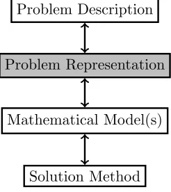
problem description and its mathematical model is not clear. Therefore an intermediate step

is included in the optimization approach (see Figure 2.1). In this step, the representation

used is detailed and approximations are made. For instance, in the context of scheduling

problems, using a discrete-time formulation is in general a constraining approximation of

the actual problem, and thus, it may lead to a suboptimal solution as discussed in Floudas

and Lin (2004).

Additionally, it is important to note that several mathematical models may be used

to obtain the global optimal solution of the problem, which is the best possible solution

according to a given optimization criterion. For example, many time representations rely

on a specific parameter representing the number of time points (Kondili et al., 1993), time

intervals (Lee et al., 1996), or event points (Ierapetritou and Floudas, 1998). Therefore, the

scheduling problem is represented by an infinite set of mathematical models, one for each

possible value of this parameter (all positive integers). The global optimal schedule is the

(34)

2.1 Introduction

Problem Description

Problem Representation

Mathematical Model(s)

Solution Method

Figure 2.1: Four steps optimization approach.

to know a priori the parameter value that will lead to the global optimal solution, although

it is sometimes possible to derive upper and lower bounds for it. The common trade-off is

that global optimality may be guaranteed with a large value of this parameter, which often

results in prohibitive solution times.

Many different time representations have been introduced to solve scheduling problems

(for review see Floudas and Lin, 2004). Experience has shown that, depending on the

characteristics of the problem, some time representations are more suitable than others. In

this thesis, we focus on scheduling problems that rely on:

a) a set of possibleoperations, or actions, that can be performed once, several times, or

not at all;

b) scheduling decisions that involve both selecting, parametrizing and sequencing the

operations that should be executed;

c) scheduling constraints such as release dates, due dates, bounds on processing times,

non-overlapping constraints, sequence-dependent changeovers, cardinality constraints,

and precedence constraints;

d) additional side constraints that are used to model more complex features such as

limited inventory management or process constraints.

It should be noted that, for instance, the selection of operations may correspond to the

(35)

2.2 Case Study

1993) or in a resource-task-network (Pantelides, 1994). In general, operations are defined

by fully disaggregating all possible discrete selections of actions in the scheduling system.

In contrast, parameterization of operations corresponds to continuous decisions such as

batch sizes, transfer volumes, or process operating conditions. The above assumptions do

not cover all kinds of scheduling problems but are an important part of the classification

presented by M´endez et al. (2006a). A unique aspect of this work is that the unifying

framework of the models presented in this chapter allows it to be applied to single-stage

and multi-stage batch scheduling problems as well as to crude-oil operations scheduling

(see chapters 3 and 4).

The main objective of this chapter is to develop a unified modeling approach for scheduling

problems in order to facilitate the evaluation of several time representations, both in terms of

computational time and solution quality. First, a simple scheduling problem is introduced

as an example. Next, we study four different types of time representations, which have

been used in the literature and clarify the relationships between them. Then, basic MILP

models for pure scheduling constraints are presented for each of these time representation.

Using concepts from graph theory (cliques and bicliques), we show how these models can be

generically strengthened based on the structure of the scheduling problem. Three solution

methods are then developed to solve these mathematical formulations. Finally, single-stage

and multi-stage batch scheduling problems are presented and solved using the different

approaches in order to show the effectiveness of the strengthened formulations, and to

provide elements of comparison between the different time representations.

2.2 Case Study

We introduce a small scheduling system that involves 6 different operationsv1, . . . , v6 and

3 unary resourcesr1, r2, r3. A unary resource cannot be shared by two or more processing

operations at a given time. Table 2.1 displays resource requirement for each operation.

(36)

2.3 Time Representations

Table 2.1: Resource requirements for case study.

Operation v1 v2 v3 v4 v5 v6

Resources r1 r2 r3 r1∧r2 r1∧r3 r2∧r3

in the examples studied in this thesis, unary resource requirements are handled as

non-overlapping constraints between operations. For instance, operations v1 and v4 cannot

overlap as they both use resource r1. Also, operations v5 and v6 cannot overlap as they

both use resource r3. Besides, as a given operation v can be executed several times, any

two separate executions ofv may not overlap. Thus, any operation v cannot overlap with

itself. Different linear objectives can be considered: maximization of profit, minimization

of makespan, minimization of assignment costs, minimization of tardiness or earliness.

In order to extract useful information from the structure of the problem, we use a global

representation of all the non-overlapping constraints. The non-overlapping matrix,

de-noted by N O, is such that N Ovv′ = 1 if operation v and v′ must not overlap, 0

oth-erwise. The non-overlapping graph, denoted by GN O = (W, E), is an undirected graph

where the set of vertices W is the set of operations and the set of edges is defined by

E ={{v, v′_} _s.t. _{N O}

vv′ = 1}. Therefore, the non-overlapping matrix is the adjacency

ma-trix of graphGN O. The concept of non-overlapping graph can be viewed as an extension of

the disjunctive graph (Balas, 1969; Adams et al., 1988), which is used to represent

disjunc-tive constraints between operations that have to be executed exactly once. In this thesis,

we consider operations that can be executed once, several times, or not at all. Figure 2.2

shows the non-overlapping matrix and graph for the case study. For clarity, edges that

connect a vertex to itself, called self-loops, are not represented.

2.3 Time Representations

In this section, we study four different time representations and show how they can be

defined using identical concepts. Each representation makes use of a totally ordered set

(37)

op-2.3 Time Representations

Figure 2.2: Non-overlapping matrix and graph for case study.

erations. The number of priority-slots, denoted by n, has to be postulated a priori. Any

operation may be executed several times by assigning it to multiple priority-slots. We

de-note by A = {(i, v), i∈ T, v ∈ W} the set of all possible assignments and define a partial

scheduling order onA by:

∀(i1, v1),(i2, v2)∈A, (i1, v1)≺(i2, v2)⇔i1< i2∧N Ov1v2 = 1

In each time representation, a solution is defined as a subset A′ of A and is represented

by a sequence of operations. Each selected assignment (i, v) correspond to an execution of

operationvwith scheduling priorityiduring time interval [Siv, Eiv]. In each time

represen-tation, the partial scheduling order ≺implies precedence relations between elements of A′

as follows:

∀(i1, v1),(i2, v2)∈A′, (i1, v1)≺(i2, v2)⇒Ei1v1 ≤Si2v2

It is should be noted that it is not straightforward to select the number of priority-slots.

Indeed, postulating a large number priority-slots increases the chance of obtaining the global

optimal solution, but it also increases the size of the model and the CPU time. The four

time representations are listed below.

a. Multi Operation Sequencing (MOS)

b. Multi Operation Sequencing with Synchronized Start Times (MOS-SST)

c. Multi Operation Sequencing with Fixed Start Times (MOS-FST)

(38)

a. MOS (continuous-time) b. MOS-SST (continuous-time)

1

c. MOS-FST (discrete-time) d. SOS (continuous-time)

1

Figure 2.3: A unique schedule obtained through different time representations.

Figure 2.3 shows how the same schedule for the case study can be obtained within each

time representations. Each execution of an operation is represented by an horizontal bar

in the upper Gantt chart, while resource usage is represented by horizontal lines in the

lower Gantt chart. The priority-slots are represented by number labels on each operation

execution. In each case, the smallest possible number of priority-slots needed to obtained

the solution has been used. From this figure, it is clear that some time representations

require more priority-slots than others.

In the MOS representation, several operations can be assigned to each priority-slots as

(39)

are allowed to overlap and are both assigned to the first priority-slot. However, operations

v1 and v5 cannot overlap and are consequently assigned to different priority-slots: slots 1

and 4 for operation v1, slot 2 for operation v5. If two non-overlapping operations v and v′

are assigned to priority-slots iand j, respectively, such that i < j, then operationv′ must

be executed after operation v (i.e. operation v must start after the end of operation v).

For instance, operationv1 assigned to priority-slot 4 is executed after operationv2 assigned

to priority-slot 2. The solution depicted in Figure 2.3(a) is represented by the sequence

of operations ({1,6},{2,5},{3,4},{1}). We denote MOS(n) a scheduling model using

the MOS time representation with n postulated priority-slots. This time representation

was introduced by Ierapetritou and Floudas (1998) as the event point formulation. Their

mathematical model, although significantly different than the model developed in this thesis,

was used to solve several STN problems. As mentioned by Maravelias and Grossmann

(2003), inventory tracking using event points is quite different than inventory tracking using

time points, which might lead to inconsistent enforcement of storage capacity constraints.

This issue was addressed by Janak et al. (2004) by adding additional storage tasks in the

STN problem, which can lead to a significant increase of model size.

TheMOS-SSTrepresentation is based on the same features as the MOS representation.

Additionally, all operations assigned to the same priority-slot must have the same start

time. For instance, in Figure 2.3(b), operationsv1 and v6 are both assigned to priority-slot

1, and therefore both start at the same time t= 0. Thus, each priority-slot iis associated

to variable time-pointti which is represented by a vertical dotted line in Figure 2.3(b). The

time interval between any two successive time-points is variable. The solution depicted in

Figure 2.3(a) is represented by the sequence of operations ({1,6},{2},{5},{3},{4},{1}).

We denote MOS-SST(n) a scheduling model using the MOS-SST time representation

withn postulated priority-slots. This type of representation has been used to solve a wide

variety of problems where time-points are used to track both the start and end events of

each operation (see Zhang and Sargent, 1996; Schilling and Pantelides, 1996; Maravelias

(40)

The MOS-FST representation is based on the same features as the MOS-SST

repre-sentation. Additionally, the time-point associated to each priority-slot is fixed a priori.

Thus, the interval between any two successive time-points is fixed. For instance, the

so-lution depicted in Figure 2.3(c) is obtained using time-points that are uniformly spaced

along the time horizon: t1 = 0, t2 = 1, . . . , t10 = 9. Therefore, operation v5 assigned to

priority-slot 4 starts at t = t4 = 3 while operation v4 assigned to priority-slot 7 starts at

t = t7 = 6. The solution depicted in Figure 2.3(c) is represented by the sequence of

op-erations ({1,6},∅,∅,{5},{2},{3},{4},∅,{1},∅). We denote MOS-FST(n) a scheduling

model using the MOS-FST time representation withn postulated priority-slots.

Discrete-time formulation for process scheduling problems were initially developed to solve STN and

RTN models where processing times are assumed to be constant (see Kondili et al., 1993;

Pantelides, 1994).

In the SOS representation, at most one operation can be assigned to each

priority-slot. Similarly to the MOS model, if two non-overlapping operations v and v′ are assigned

to priority-slots i and j (i < j), then v′ _{must be executed after} _v_{. It should be noted}

that this constraint does not apply to pairs of operations that are allowed to overlap. As

operations v2 and v5 are allowed to overlap, their relative position in time is not affected

by their respective scheduling priority. Therefore, the proposed solution is equivalent to

assigning operationsv2 and v5 to priority-slots 4 and 3, respectively. The solution depicted

in Figure 2.3(d) is represented by the sequence of operations (1,6,2,5,3,4,1). We denote

SOS(n) a scheduling model using the SOS time representation withn postulated

priority-slots. This time representation was introduced by Mouret et al. (2009a) to solve the refinery

crude-oil operations scheduling problem.

Table 2.2 summarizes the correspondence between our nomenclature and equivalent

nam-ing conventions used in the literature. From these definitions, it can be inferred that for

a given number of priority-slots n the integer feasible space of MOS(n) is larger than

the integer feasible space of modelsMOS-SST(n),MOS-FST(n), andSOS(n). Indeed,

(41)

Table 2.2: Time representations nomenclature.

Nomenclature Equivalent names

MOS unit-specific time grid or multiple time grid

MOS-SST global events or common time grid or nonuniform discretization

MOS-FST fixed events or fixed time grid or uniform discretization

SOS first introduced in Mouret et al. (2009a)

which reduce the set of feasible solutions. Furthermore, the integer feasible space of

MOS-SST(n) is larger than the one of MOS-FST(n) and SOS(n). In particular, any solution

for theSOS model is a solution for theMOS-SST model. Indeed, at most one operation

can be assigned to each priority-slot so the synchronization of start times is automatically

satisfied.

These properties can also be interpreted by considering a scheduling solution z. We

denote z ∈ MOS(n) the membership of schedule z to the integer feasible space of model

MOS(n). In other words, z∈MOS(n) means that solution z satisfies all the constraints

of model MOS(n). We introduce the minimum number of priority-slots needed to ”find”

solution z using each time representation.

nMOS(z) = min

n {n|z∈MOS(n)}

nMOS-SST(z) = min

n {n|z∈MOS-SST(n)}

nMOS-FST(z) = min

n {n|z∈MOS-FST(n)}

nSOS(z) = min

n {n|z∈SOS(n)}

Then, the following inequalities hold:

 



nMOS(z)≤nMOS-SST(z)≤nMOS-FST(z)

nMOS(z)≤nMOS-SST(z)≤nSOS(z)

The relation between MOS-SST and MOS-FST time representations was previously

de-rived by Maravelias and Grossmann (2006) in the context of state-task network formulations.

Remark. An important limitation of these time representations is that operations are

(42)

2.4 Mathematical Models

assigned to operations and not to the start and end events of these operations, which may

be necessary to solve some scheduling problems. For instance, operations that require a

cumulative resource with capacity greater than 1 (e.g. manpower limited to 2 workers) are

allowed to overlap, but only a limited number of these operations may overlap at any given

point in time. The models developed in this thesis do not accommodate these features.

Another case is inventory tracking when simultaneous charging and discharging of tanks

is allowed. It is sufficient to enforce capacity limitations only at the start and end events

of each charging/discharging operations, but in order to do so, a precise sequence of such

events needs to be obtained by the model. Possible extensions of the model to handle these

specific features, such as presented in Janak et al. (2004), will not be discussed in this thesis.

2.4 Mathematical Models

In this section, we present mathematical models for each time representation. They all rely

on the same sets, parameters and variables. Objective functions are not presented here (e.g.

minimize makespan, minimize tardiness, or maximize profit) although they can significantly

impact the solution of the corresponding formulation.

2.4.1 Sets and Parameters

The following sets and parameters are used.

• T ={1, . . . , n} is a totally ordered set of priority-slots (indicesi, j, i1, i2).

• W is the set of all operations (indicesv, v′, v1, v2).

• H is the scheduling horizon.

• [Sv, Sv]⊂[0, H] are bounds on the start time of any execution of operationv.

• [Dv, Dv]⊂[0, H] are bounds on the duration of any execution of operationv.

• [Ev, Ev]⊂[0, H] are bounds on the end time of any execution of operation v.

• [Nv, Nv] are bounds on the total number of executions of operation v.

(43)

• N Ov1v2 is 1 if operationsv1 and v2 must not overlap, 0 if they are allowed to overlap.

• T Rv1v2 is a sequence-dependent transition time between non-overlapping operations

v1 and v2.

• T RW′ is a unique set transition time between any pair of non-overlapping operations

inW′_⊂_W_.

• Pv1v2 = 1 denotes a precedence constraint between operationsv1 and v2.

• PW1W2 = 1 denotes a precedence constraint between sets of operations W1 and W2.

Remark 1: It should be noted that for operations with fixed processing time, Dv =

Dv=Dv.

Remark 2: A set transition timeT RW′ is defined when∀v₁, v₂ ∈W′, T R_v₁_,v₂ =T R_W′.

It can be used to represent unit changeover times.

Remark 3: A precedence constraint between operations v1 and v2 states that v1 must

be executed beforev2. We assume that precedence constraints are enforced on operations

which are executed exactly once (Nv1 = Nv2 = Nv1 = Nv2 = 1). Similarly, we consider

that a precedence constraint between sets of operationsW1 and W2 states that exactly one

operation in each set must be executed (NW1 =NW2 =NW1 =NW2 = 1) and the operation

selected from W1 must be executed before the operation selected fromW2.

2.4.2 Variables

The variables used in all models are composed of binary assignment variables, and

contin-uous time variables.

• Assignment variablesZiv ∈ {0,1} i∈T, v ∈W

Ziv= 1 if operationv is assigned to priority-slot i,Ziv= 0 otherwise.

• Time variablesSiv≥0, Div≥0, Eiv≥0 i∈T, v∈W

Sivis the start time of operationvif it is assigned to priority-sloti,Siv= 0 otherwise.

Div is the duration of operationvif it is assigned to priority-sloti,Div= 0 otherwise.

(44)

2.4.3 MOS Model

Variable Bound Constraints Bounds on time variables can be expressed using the

following constraints.

Sv·Ziv ≤Siv≤Sv·Ziv i∈T, v∈W (2.1a)

Dv·Ziv≤Div≤Dv·Ziv i∈T, v∈W (2.1b)

Ev·Ziv ≤Eiv≤Ev·Ziv i∈T, v∈W (2.1c)

Time Constraint Time variables are linked through the following additional constraint.

Eiv=Siv+Div i∈T, v∈W (2.2)

Cardinality constraint The total number of execution of operations in a set W′ _⊂_W

is restricted by the following constraint. A cardinality constraint on a single operation v

can be enforced by setting W′₌_{_v_}.

NW′ ≤

X

i∈T v∈W′

Ziv≤NW′ W′ ⊂W (2.3)

Assignment Constraint Two non-overlapping operationsv1andv2such thatN Ov1v2 =

1 cannot be assigned simultaneously to the same priority-slot.

Ziv1 +Ziv2 ≤1 i∈T, v1, v2 ∈W, N Ov1v2 = 1 (2.4)

Non-overlapping Constraint A non-overlapping constraint between two operations

v1, v2 ∈ W states that they must not be executed simultaneously. This property is

en-forced using the following big-M constraints where the big-M constant is defined as a valid

upper bound of the left hand side of the inequality.

Ei1v1 ≤Si2v2+H·(1−Zi2v2) i1, i2 ∈T, i1 < i2, v1, v2 ∈W, N Ov1v2 = 1 (2.5a)

Optimal Scheduling of Refinery Crude Oil Operations

Carnegie Mellon University

Research Showcase

Dissertations

Theses and Dissertations

12-1-2010

Optimal Scheduling of Refinery Crude-Oil

Operations

Sylvain Mouret

Follow this and additional works at:

http://repository.cmu.edu/dissertations

Recommended Citation

Optimal Scheduling of Refinery

Crude-Oil Operations

Acknowledgments

Abstract

Contents

List of Tables

List of Figures

Chapter 1

Introduction

1.1

Single-Stage and Multi-Stage Batch Scheduling

1.2

Optimization of Oil Refineries

Crude Vessels

Storage Tanks Charging Tanks

CDU

1

2

3

4

5

6

7

8

1.3

Mixed-Integer Optimization Tools

1.4

Overview of Thesis

Chapter 2

Time Representations and Mathematical

Models for Process Scheduling Problems

2.1

Introduction

2.2

Case Study

2.3

Time Representations

2.4

Mathematical Models