N E W J E R S E Y • L O N D O N • S I N G A P O R E • B E I J I N G • S H A N G H A I • H O N G K O N G • T A I P E I • C H E N N A I
World Scientific
Fordham University, USA
British Library Cataloguing-in-Publication Data
A catalogue record for this book is available from the British Library.
For photocopying of material in this volume, please pay a copying fee through the Copyright Clearance Center, Inc., 222 Rosewood Drive, Danvers, MA 01923, USA. In this case permission to photocopy is not required from the publisher.
ISBN-13 978-981-4313-68-1 ISBN-10 981-4313-68-8
ISBN-13 978-981-4313-69-8 (pbk) ISBN-10 981-4313-69-6 (pbk)
All rights reserved. This book, or parts thereof, may not be reproduced in any form or by any means, electronic or mechanical, including photocopying, recording or any information storage and retrieval system now known or to be invented, without written permission from the Publisher.
Copyright © 2011 by World Scientific Publishing Co. Pte. Ltd. World Scientific Publishing Co. Pte. Ltd.
5 Toh Tuck Link, Singapore 596224
USA office: 27 Warren Street, Suite 401-402, Hackensack, NJ 07601
UK office: 57 Shelton Street, Covent Garden, London WC2H 9HE
Printed in Singapore.
In high school, I used to like geometry better than algebra or arithmetic. I became excited about matrix algebra after my teacher at Harvard, Pro-fessor Wassily Leontief, Nobel laureate in Economics showed me how his input-output analysis depends on matrix inversion. Of course, inverting a 25×25 matrix was a huge deal at that time. It got me interested in com-puter software for matrix algebra tasks. This book brings together my two fascinations, matrix algebra and computer software to make the algebraic results fun to use, without the drudgery of patient arithmetic manipula-tions.
I was able to find a flaw in Nobel Laureate Paul Samuelson’s published work by pointing out that one of his claims for matrices does not hold for scalars. Further excitement came when I realized that Italian economist Sraffa’s work, extolled in Professor Samuelson’s lectures can be understood better in terms of eigenvectors. My interest about matrix algebra further increased when I started working at Bell Labs and talking to many engineers and scientists. My enthusiasm for matrix algebra increased when I worked with my friend Sharad Sathe on our joint paper Sathe and Vinod (1974). My early publication in Econometrica on joint production, Vinod (1968), heavily used matrix theory. My generalization of the Durbin-Watson test in Vinod (1973) exploited the Kronecker product of matrices. In other words, a study of matrix algebra has strongly helped my research agenda over the years.
Research oriented readers will find that matrix theory is full of useful results, ripe for applications in various fields. The hands-on approach here using the R software and graphics hopes to facilitate the understanding of results, making such applications easy to accomplish. An aim of this book is to facilitate and encourage such applications.
The primary motivation for writing this book has been to make learning of matrix algebra fun by using modern computing tools in R. I am assuming that the reader has very little knowledge of R and am providing some help with learning R. However, teaching R is not the main purpose, since on-line free manuals are available. I am providing some tips and hints which may be missed by some users of R. For something to be fun, there needs to be a reward at the end of an effort. There are many matrix algebra books for those purists who think learning matrix algebra is a reward in itself. We take a broader view of a researcher who wants to learn matrix algebra as a tool for various applications in sciences and engineering. Matrices are important in statistical data analysis. An important reference for Statistics using matrix algebra is Rao (1973).
This book should appeal to the new generation of students, “wired dif-ferently” with digitally nimble hands, willing to try difficult concepts, but less skilled with arithmetic manipulations. I believe this generation may not have a great deal of patience with long tedious manipulations. This book shows how they can readily create matrices of any size and satisfy-ing any properties in R with random entries and then check if any alleged matrix theory result is plausible. A fun example of Fibonacci numbers is used in Sec. 17.1.3 to illustrate inaccuracies in floating point arithmetic of computers. It should be appealing to the new generation, since many nat-ural (biological) phenomena follow the pattern of these numbers, as they can readily check on Google.
This book caters to students and researchers who do not wish to empha-size proofs of algebraic theorems. Applied people often want to ‘see’ what a theorem does and what it might mean in the context of several exam-ples, with a view to applying the theorem as a practical tool for simplifying or deeply understanding some data, or for solving some optimization or estimation problem.
For example, consider the familiar regression model
y=Xβ+ǫ, (0.1)
in matrix notation, where y is a T ×1 vector, X is T ×p matrix, β is a p×1 vector and ε is T ×1 vector. In statistics it is well known that
b= (X′X)−1X′y is the ordinary least squares (OLS) estimator minimizing
error sum of squaresε′ε.
theorems show that when a ‘singular value’ is close to zero, the matrix of regressors is ‘ill-conditioned’ and regression computations and statisti-cal inference based on computed estimates are often unreliable. See Vinod (2008a, Sec. 1.9) for econometric examples and details.
The book does not shy away from mentioning applications making purely matrix algebraic concepts like the SVD alive. I hope to provide a motivation for learning them as in Chapter 16. Section 16.8 in the same Chapter uses matrix algebra and R software to expose flaws in the popu-lar Hodrick-Prescott filter, commonly used for smoothing macroeconomic time series to focus on underlying business cycles. Since the flaw cannot be ‘seen’ without the matrix algebra used by Phillips (2010) and implemented in R, it should provide further motivation for learning both matrix algebra and R. Even pure mathematicians are thrilled when their results come alive in R implementations and find interesting applications in different applied scientific fields.
Now I include some comments on the link between matrix algebra and computer software. We want to use matrix algebra as a tool for a study of some information and data. The available information can be seen in any number of forms. These days a familiar form in which the information might appear is as a part of an ‘EXCEL’ workbook popular with practitioners who generally need to deal with mixtures of numerical and character values including names, dates, classification categories, alphanumeric codes, etc. Unfortunately EXCEL is good as a starting point, but lacks the power of R.
Matrix algebra is a branch of mathematics and cannot allow fuzzy think-ing involvthink-ing mixed content. Its theorems cannot apply to mixed objects without important qualifications. Traditional matrices usually deal with purely numerical content. In R traditional algebraic matrices are objects called ‘matrix,’ which are clearly distinguished from similar mixed objects needed by data analysts called ‘data frames.’ Certain algebraic operations on rows and columns can also make sense for data frames, while not others. For example, the ‘summary’ function summarizes the nature of information in a column of data and is a very fundamental tool in R.
can initially learn what a particular column has, by using the ‘summary’ on the data frame.
This book will also review results related to matrix algebra which are rel-evant for numerical analysts. For example, inverting ill-conditioned sparse matrices and error propagation. We cover several advanced topics believed to be relevant for practical applications. I have attempted to be as com-prehensive as possible, with a focus on potentially useful results. I thank following colleagues and students for reading and suggesting improvements to some chapters of an earlier version: Shapoor Vali, James Santangelo, Ahmad Abu-Hammour, Rossen Trendafilov and Michael Gallagher. Any remaining errors are my sole responsibility.
Preface vii
1. R Preliminaries 1
1.1 Matrix Defined, Deeper Understanding Using Software . . 1
1.2 Introduction, Why R? . . . 2
1.3 Obtaining R . . . 4
1.4 Reference Manuals in R . . . 5
1.5 Basic R Language Tips . . . 6
1.6 Packages within R . . . 12
1.7 R Object Types and Their Attributes . . . 17
1.7.1 Dataframe Matrix and Its Summary . . . 18
2. Elementary Geometry and Algebra Using R 21 2.1 Mathematical Functions . . . 21
2.2 Introductory Geometry and R Graphics . . . 22
2.2.1 Graphs for Simple Mathematical Functions and Equations . . . 25
2.3 Solving Linear Equation by Finding Roots . . . 27
2.4 Polyroot Function in R . . . 29
2.5 Bivariate Second Degree Equations and Their Plots . . . 32
3. Vector Spaces 41 3.1 Vectors . . . 41
3.1.1 Inner or Dot Product and Euclidean Length or Norm 42 3.1.2 Angle Between Two Vectors, Orthogonal Vectors 43 3.2 Vector Spaces and Linear Operations . . . 46
3.2.1 Linear Independence, Spanning and Basis . . . 47
3.2.2 Vector Space Defined . . . 49
3.3 Sum of Vectors in Vector Spaces . . . 50
3.3.1 Laws of Vector Algebra . . . 52
3.3.2 Column Space, Range Space and Null Space . . . 52
3.4 Transformations of Euclidean Plane Using Matrices . . . . 52
3.4.1 Shrinkage and Expansion Maps . . . 52
3.4.2 Rotation Map . . . 53
3.4.3 Reflexion Maps . . . 53
3.4.4 Shifting the Origin or Translation Map . . . 54
3.4.5 Matrix to Compute Deviations from the Mean . . 54
3.4.6 Projection in Euclidean Space . . . 55
4. Matrix Basics and R Software 57 4.1 Matrix Notation . . . 57
4.1.1 Square Matrix . . . 60
4.2 Matrices Involving Complex Numbers . . . 60
4.3 Sum or Difference of Matrices . . . 61
4.4 Matrix Multiplication . . . 63
4.5 Transpose of a Matrix and Symmetric Matrices . . . 66
4.5.1 Reflexive Transpose . . . 66
4.5.2 Transpose of a Sum or Difference of Two Matrices 67 4.5.3 Transpose of a Product of Two or More Matrices 67 4.5.4 Symmetric Matrix . . . 68
4.5.5 Skew-symmetric Matrix . . . 69
4.5.6 Inner and Outer Products of Matrices . . . 71
4.6 Multiplication of a Matrix by a Scalar . . . 72
4.7 Multiplication of a Matrix by a Vector . . . 73
4.8 Further Rules for Sum and Product of Matrices . . . 74
4.9 Elementary Matrix Transformations . . . 76
4.9.1 Row Echelon Form . . . 80
4.10 LU Decomposition . . . 80
5. Decision Applications: Payoff Matrix 83 5.1 Payoff Matrix and Tools for Practical Decisions . . . 83
5.2 Maximax Solution . . . 85
5.3 Maximin Solution . . . 86
5.5 Digression: Mathematical Expectation from Vector
Multi-plication . . . 89
5.6 Maximum Expected Value Principle . . . 90
5.7 General R Function ‘payoff.all’ for Decisions . . . 92
5.8 Payoff Matrix in Job Search . . . 95
6. Determinant and Singularity of a Square Matrix 99 6.1 Cofactor of a Matrix . . . 101
6.2 Properties of Determinants . . . 103
6.3 Cramer’s Rule and Ratios of Determinants . . . 108
6.4 Zero Determinant and Singularity . . . 110
6.4.1 Nonsingularity . . . 113
7. The Norm, Rank and Trace of a Matrix 115 7.1 Norm of a Vector . . . 115
7.1.1 Cauchy-Schwartz Inequality . . . 116
7.2 Rank of a Matrix . . . 116
7.3 Properties of the Rank of a Matrix . . . 118
7.4 Trace of a Matrix . . . 121
7.5 Norm of a Matrix . . . 123
8. Matrix Inverse and Solution of Linear Equations 127 8.1 Adjoint of a Matrix . . . 127
8.2 Matrix Inverse and Properties . . . 128
8.3 Matrix Inverse by Recursion . . . 132
8.4 Matrix Inversion When Two Terms Are Involved . . . 132
8.5 Solution of a Set of Linear EquationsAx=b . . . 133
8.6 Matrices in Solution of Difference Equations . . . 135
8.7 Matrix Inverse in Input-output Analysis . . . 136
8.7.1 Non-negativity in Matrix Algebra and Economics 140 8.7.2 Diagonal Dominance . . . 141
8.8 Partitioned Matrices . . . 142
8.8.1 Sum and Product of Partitioned Matrices . . . 143
8.8.2 Block Triangular Matrix and Partitioned Matrix Determinant and Inverse . . . 143
8.9 Applications in Statistics and Econometrics . . . 147
8.9.3 Simultaneous Equation Models . . . 151
8.9.4 Haavelmo Model in Matrices . . . 153
8.9.5 Population Growth Model from Demography . . . 154
9. Eigenvalues and Eigenvectors 155 9.1 Characteristic Equation . . . 155
9.1.1 Eigenvectors . . . 157
9.1.2 nEigenvalues . . . 158
9.1.3 nEigenvectors . . . 158
9.2 Eigenvalues and Eigenvectors of Correlation Matrix . . . . 159
9.3 Eigenvalue Properties . . . 161
9.4 Definite Matrices . . . 163
9.5 Eigenvalue-eigenvector Decomposition . . . 164
9.5.1 Orthogonal Matrix . . . 166
9.6 Idempotent Matrices . . . 168
9.7 Nilpotent and Tripotent matrices . . . 172
10. Similar Matrices, Quadratic and Jordan Canonical Forms 173 10.1 Quadratic Forms Implying Maxima and Minima . . . 173
10.1.1 Positive, Negative and Other Definite Quadratic Forms . . . 176
10.2 Constrained Optimization and Bordered Matrices . . . 178
10.3 Bilinear Form . . . 179
10.4 Similar Matrices . . . 179
10.4.1 Diagonalizable Matrix . . . 180
10.5 Identity Matrix and Canonical Basis . . . 180
10.6 Generalized Eigenvectors and Chains . . . 181
10.7 Jordan Canonical Form . . . 182
11. Hermitian, Normal and Positive Definite Matrices 189 11.1 Inner Product Admitting Complex Numbers . . . 189
11.2 Normal and Hermitian Matrices . . . 191
11.3 Real Symmetric and Positive Definite Matrices . . . 197
11.3.1 Square Root of a Matrix . . . 200
11.3.2 Positive Definite Hermitian Matrices . . . 200
11.3.3 Statistical Analysis of Variance and Quadratic Forms . . . 201
11.4 Cholesky Decomposition . . . 205
11.5 Inequalities for Positive Definite Matrices . . . 207
11.6 Hadamard Product . . . 207
11.6.1 Frobenius Product of Matrices . . . 208
11.7 Stochastic Matrices . . . 209
11.8 Ratios of Quadratic Forms, Rayleigh Quotient . . . 209
12. Kronecker Products and Singular Value Decomposition 213 12.1 Kronecker Product of Matrices . . . 213
12.1.1 Eigenvalues of Kronecker Products . . . 220
12.1.2 Eigenvectors of Kronecker Products . . . 221
12.1.3 Direct Sum of Matrices . . . 222
12.2 Singular Value Decomposition (SVD) . . . 222
12.2.1 SVD for Complex Number Matrices . . . 226
12.3 Condition Number of a Matrix . . . 228
12.3.1 Rule of Thumb for a Large Condition Number . . 228
12.3.2 Pascal Matrix is Ill-conditioned . . . 229
12.4 Hilbert Matrix is Ill-conditioned . . . 230
13. Simultaneous Reduction and Vec Stacking 233 13.1 Simultaneous Reduction of Two Matrices to a Diagonal Form . . . 233
13.2 Commuting Matrices . . . 234
13.3 Converting Matrices Into (Long) Vectors . . . 239
13.3.1 Vec ofABC . . . 241
13.3.2 Vec of (A+B) . . . 243
13.3.3 Trace ofABIn Terms of Vec . . . 244
13.3.4 Trace ofABC In Terms of Vec . . . 245
13.4 Vech for Symmetric Matrices . . . 247
14. Vector and Matrix Differentiation 249 14.1 Basics of Vector and Matrix Differentiation . . . 249
14.2 Chain Rule in Matrix Differentiation . . . 254
14.2.1 Chain Rule for Second Order Partials wrtθ . . . 254
14.2.2 Hessian Matrices in R . . . 255
14.2.3 Bordered Hessian for Utility Maximization . . . . 255
14.3 Derivatives of Bilinear and Quadratic Forms . . . 256
14.4.1 Derivatives of a Quadratic Form wrtθ . . . 257
14.4.2 Derivatives of a Symmetric Quadratic Form wrtθ 258 14.4.3 Derivative of a Bilinear form wrt the Middle Matrix . . . 258
14.4.4 Derivative of a Quadratic Form wrt the Middle Matrix . . . 258
14.5 Differentiation of the Trace of a Matrix . . . 258
14.6 Derivatives oftr(AB),tr(ABC) . . . 259
14.6.1 Derivativetr(An) wrt AisnA−1 . . . 261
14.7 Differentiation of Determinants . . . 261
14.7.1 Derivative oflog(det A) wrtAis (A−1)′ . . . 261
14.8 Further Derivative Formulas for Vec andA−1 . . . 262
14.8.1 Derivative of Matrix Inverse wrt Its Elements . . 262
14.9 Optimization in Portfolio Choice Problem . . . 262
15. Matrix Results for Statistics 267 15.1 Multivariate Normal Variables . . . 267
15.1.1 Bivariate Normal, Conditional Density and Regression . . . 272
15.1.2 Score Vector and Fisher Information Matrix . . . 273
15.2 Moments of Quadratic Forms in Normals . . . 274
15.2.1 Independence of Quadratic Forms . . . 276
15.3 Regression Applications of Quadratic Forms . . . 276
15.4 Vector Autoregression or VAR Models . . . 276
15.4.1 Canonical Correlations . . . 277
15.5 Taylor Series in Matrix Notation . . . 278
16. Generalized Inverse and Patterned Matrices 281 16.1 Defining Generalized Inverse . . . 281
16.2 Properties of Moore-Penrose g-inverse . . . 283
16.2.1 Computation of g-inverse . . . 284
16.3 System of Linear Equations and Conditional Inverse . . . 287
16.3.1 Approximate Solutions to Inconsistent Systems . 288 16.3.2 Restricted Least Squares . . . 289
16.4 Vandermonde and Fourier Patterned Matrices . . . 290
16.4.1 Fourier Matrix . . . 292
16.4.2 Permutation Matrix . . . 293
16.4.4 Nonnegative Indecomposable Matrices . . . 293
16.4.5 Perron-Frobenius Theorem . . . 294
16.5 Diagonal Band and Toeplitz Matrices . . . 294
16.5.1 Toeplitz Matrices . . . 295
16.5.2 Circulant Matrices . . . 296
16.5.3 Hankel Matrices . . . 297
16.5.4 Hadamard Matrices . . . 298
16.6 Mathematical Programming and Matrix Algebra . . . 299
16.7 Control Theory Applications of Matrix Algebra . . . 300
16.7.1 Brief Introduction to State Space Models . . . 300
16.7.2 Linear Quadratic Gaussian Problems . . . 301
16.8 Smoothing Applications of Matrix Algebra . . . 303
17. Numerical Accuracy and QR Decomposition 307 17.1 Rounding Numbers . . . 307
17.1.1 Binary Arithmetic and Computer Bits . . . 308
17.1.2 Floating Point Arithmetic . . . 308
17.1.3 Fibonacci Numbers Using Matrices and Digital Computers . . . 309
17.2 Numerically More Reliable Algorithms . . . 312
17.3 Gram-Schmidt Orthogonalization . . . 313
17.4 The QR Modification of Gram-Schmidt . . . 313
17.4.1 QR Decomposition . . . 314
17.4.2 QR Algorithm . . . 314
17.5 Schur Decomposition . . . 318
Bibliography 321
R Preliminaries
1.1 Matrix Defined, Deeper Understanding Using Software
Scientists and accountants often use a set of numbers arranged in rectangu-lar arrays. Scientists and mathematicians call rectangurectangu-lar arrays matrices. For example, a 2×3 matrix of six numbers is defined as:
A={aij}=
a11a12a13
a21a22a23
=
3 5 11 6 9 12
, (1.1)
where the first subscript i = 1,2 of aij refers to the row number and the
second subscriptj= 1,2,3 refers to the column number.
Such matrices and their generalizations will be studied in this book in considerable detail. Rectangular arrays of numbers are called spreadsheets or workbooks in accounting parlance and ‘Excel’ software has standardized them in recent decades. The view of rectangular arrays of numbers by different professions can be unified. The aim of this book is to provide tools for developing a deeper understanding of the reality behind rectangular arrays of numbers by applying many powerful results of matrix algebra along with certain software and graphics tools.
Exercise 1.1.1: Construct a 2×2 matrix with elements aij = i+j.
[Hint: the first row will have numbers 2,3 and second row will have 3,4].
Exercise1.1.2: Given integers 1 to 9 construct a 3×3 matrix with first row having numbers 1 to 3, second row with numbers 4 to 6 and last row with numbers 7 to 9.
The R software allows a unified treatment of all rectangular arrays as ‘data frame’ objects. Although matrix algebra theorems do not directly apply to data frames, they are a useful preliminary, allowing matrix algebra to be a very practical and useful tool in everyday life, not some esoteric subject for scientists and mathematicians. For one thing, the data frame
objects in R software allow us to name the rows and columns of matrices in a meaningful way. We can, of course, strip away the row-column names when treating them as matrices. Matrix algebra is abstract in the sense that its theorems hold true irrespective of row-column names. However, the deeper understanding of the reality behind those rectangular arrays of numbers requires us to have easy access to those names when we want to interpret the meaning of matrix algebra based conclusions.
1.2 Introduction, Why R?
The New York Times, 6 January 2009 had an article by Daryl Pregibon, a research scientist at Google entitled “Data Analysts Captivated by R’s Power.” It said that the software and graphics system called R is fast becoming the lingua franca of a growing number of data analysts inside corporations and academia. Countless statisticians, engineers and scientists without computer programming skills find R “easy to use.” It is hard to believe that R is free. The article also stated that “R is really important to the point that it’s hard to overvalue it.”
R is numerically one of the most accurate languages, perhaps because it is free with transparent code which can be checked for accuracy by almost anyone, anywhere. R is supported by volunteer experts from around the world and available anywhere one has access to (high speed) Internet. R works equally well on Windows, Linux, and Mac OS X computers. R is based on an earlier public domain language called S developed in Bell Labs in 1970’s. I had personally used S when I was employed at Bell Laboratories. At that time it was available only on UNIX operating system computers based on principles of object oriented languages. S-PLUS is the commercial version of S, whereas R is the free version. It is a very flexible object oriented language (OOL) in the sense that inputs, data and outputs are all objects (e.g., files) inside the computer.
shows how to get the birth day-of-the-week from a birthday of a friend. It can also give you the date and day-of-the-week 100 days before today and fun things like that. There are many data sets already loaded in R. The dataset ‘women’ contains Average Heights and Weights for American Women. The simple R command ‘summary(women)’ gives basic descriptive statistics for the data (minimum, maximum, quartiles, median and mean). No calculator can do this so conveniently. The dataset named ‘co2’ has Mauna Loa Atmospheric CO2 Concentration to check global warming. The reader will soon discover that it is more fun to use R rather than any calculator.
Actually, easy and powerful graphics capabilities of R make it fun for many of my students. The command ‘example(points)’ gives code examples showing all kinds of lines along points and creation of sophisticated symbols and shapes in R graphs. A great Internet site for all kinds of R graphics will convince anyone how much fun one can have with R:http://AddictedToR. free.fr/graphiques/index.php
The reason why R a very powerful and useful calculator is that thou-sands of ‘functions’ and program packages are already written in R. The packages are well documented in standard format and have illustrative ex-amples and user-friendly vignettes. The user simply has to know what the functions do and go ahead and use them at will, for free. Even if R is a “language” it is an “interpreted” language similar to a calculator, and the language C, not “compiled” language similar to FORTRAN, GAUSS, or similar older languages.
Similar to a calculator, all R commands are implemented as they are received by R (typed). Instead of having subroutines similar to FORTRAN, R has ‘functions.’ Calculations requiring hundreds of steps can be defined as ‘functions’ and subsequently implemented by providing values for the suitable number of arguments to these functions. A typical R package has several functions and data sets. R is functional and interpreted computer language which can readily import and employ the code for functions writ-ten in other languages including C, C++, FORTRAN, among others.
John M. Chambers, one of my colleagues at Bell Labs, is credited with creating S and helping in the creation of R. He has published an article entitled “The Future of R” in the first issue (May 2009) of the ‘R Journal’ available on the Internet at:
http://journal.r-project.org/\break2009-1/RJournal\ _2009-1\_Chambers.pdf
(i) an interface to computational procedures of many kinds; (ii) interactive, hands-on in real time;
(iii) functional in its model of programming; (iv) object-oriented, “everything is an object”;
(v) modular, built from standardized pieces; and, (vi) collaborative, a world-wide, open-source effort.
This list beautifully explains the enormous growth and power of R in recent years. Chambers goes on to explain how R functions are themselves objects with their own functionality.
I ask my students to first type a series of commands into a text editor and then copy and paste them into R. I recommend the text editor called Tinn-R, freely available at: (http://www.sciviews.org/Tinn-R/). The reader should go to the bottom of the web page and download it to his or her computer. Next, click on “Setup for Tinn-R” Be sure to use the old stable version (1.17.2.4) (.exe, 5.2 Mb) compatible with Rgui in SDI or MDI mode. Tinn-R color codes the R commands and provides helpful hints regarding R syntax in the left column entitled ‘R-card.’ Microsoft Word is also a good text editor to use, but care is needed to avoid smart or slanted quotation marks (unknown to R).
1.3 Obtaining R
One can Google the word r-project and get the correct Internet address. The entire software is ‘mirrored’ or repeated at several sites on the Internet around the world. One can go to
(http://www.r-project.org) and choose a geographically nearby mir-ror. For example, US users can choose
http://cran.us.r-project.org
Once arriving at the appropriate Internet site, one looks on the left hand side under “Download.” Next, click on CRAN Link. Sometimes the site asks you to pick a mirror closest to your location again. Click on ‘Windows’ (if you have a Windows computer) and then Click on ‘base.’
will first ask you language, choose English. Then click ‘Next’ and follow other on-screen instructions.
If you have a Windows Vista computer, among frequently asked ques-tion, they have answer to the question: How do I install R when using Windows Vista? One of the hints is ‘Run R with Administrator privileges in sessions where you want to install packages.’
Choose simple options. Do not customize it. The setup does every-thing, including creating an Icon for R-Gui (graphical user interface). It immediately lets you know what version is being used.
1.4 Reference Manuals in R
Starting at the R website (http://cran.r-project.org) left column click on ‘manuals’ and access the first bullet point called “An Introduction to R,” which is the basic R manual with about 100 pages. It can be browsed in html format at:
http://cran.r-project.org/doc/manuals/R-intro.html
It can also be downloaded in the pdf format by clicking at a link within that bullet as:
http://cran.r-project.org/doc/manuals/R-intro.pdf
The reader is encouraged to read all chapters, especially Chapter 5 of ‘R-intro’ dealing with arrays and Chapter 12 dealing with graphics.
There are dozens of free books available on the Internet about R at: http://cran.r-project.org/doc/contrib
The books are classified into 12 books having greater than 100 pages starting with “Using R for Data Analysis and Graphics - Introduction, Examples and Commentary” by John Maindonald. Section 7.8 of the above pdf file deals specifically with matrices and arrays in R.
http://cran.r-project.org/doc/contrib/usingR.pdf
There are additional links to some 18 (as of July 2009) short books (having less than 100 pages). The list starts with “R for Beginners” by Emmanuel Paradis.
use R.
1.5 Basic R Language Tips
Of course, the direct method of learning any language is to start using it. I recommend learning the assignment symbols ‘=’ or ‘<-’ and the combine symbol ‘c’ and start using R as a calculator. A beginning user of R should consult one or more of the freely available R manuals mentioned in Sec. 1.4. Nevertheless, this section lists some practical points useful to beginning users, as well as, some experienced users of R.
(i) Unlike paper and pencil mathematics, (*) means multiply; either the hat symbol ( ∧) or (∗∗) are used for raising to a power; (|) means the logical ‘or’ and (!) means logical negation.
(ii) If a command is inside simple parentheses (not brackets) it is printed to the screen.
(iii) Colon (:) means generate a sequence. For example, x=3:7 creates an R (list or vector) object named ‘x’ containing the numbers (3,4,5,6,7). (iv) Generally speaking, R ignores all spaces inside command lines. For
example, ‘x=1:3’ is the same as ‘x = 1 : 3’.
(v) Comments within R code are put anywhere, starting with a hash-mark (‘#’), such that everything from that point to the end of the line is a comment by the author of the code (usually to oneself) and completely ignored by the R processor.
(vi) ‘c’ is a very important and very basic function in R which combines its arguments. One cannot really use R without learning to use the ‘c’ function. For example, ‘x=c(1:5, 17, 99)’ will create a ‘vector’ or a ‘list’ object called ‘x’ with elements: (1, 2, 3, 4, 5, 17, 99). The ‘c’ stands for ‘concatenate’, ‘combine’ or ‘catalog.’
(vii) Generally, each command should be on a separate line of code. If one wants to type or have two or more commands on one line, a semi-colon (;) must be used to separate them.
(viii) R is case sensitive similar to UNIX. For example, the lower case named object b is different from upper case named object B.
(ix) The object names usually start with a letter, never with numbers. Spe-cial characters including underscores are not allowed in object names but periods (.) are allowed.
*, / and the hat symbol (∧) for raising to a power are available. R also has log, exp, sin, cos, tan, sqrt, min, max with self-explanatory meanings.
(xi) Expressions and assignments are distinct in R. For example, if you type the expression:
2+3+4^2
R will proceed to evaluate it. If you assign the expression a name ‘x’ by typing:
x=2+3+4^2; x
The resulting object called ‘x’ will contain the evaluation of the expres-sion and will be available under the name ‘x,’ but not automatically printed to the screen. Assuming that one wants to see R print it, one needs to type ‘x’ or ‘print(x)’ as a separate command. We have in-cluded ‘x’ after the semi-colon (;) to suggest a new command asking R to print the result to the screen.
(xii) The R language and its packages together have tens of thousands of functions for doing certain tasks on their arguments. For example, ‘sqrt’ is a function in R which computes the square root of its argu-ment. It is important to use simple parentheses as in ‘print(x)’ or ‘sqrt(x)’ when specifying the arguments of R functions. Using curly braces or brackets instead of parentheses will give syntax error (or worse confusion) in R.
(xiii) Brackets are used to extract elements of an array. For example, ‘x[2]’ extracts second element of a list ‘x’. Similarly, ‘x[2,1]’ extracts the number along the second row and first column of a matrix x. Again, using curly braces or parentheses will not work for this purpose. (xiv) Curly braces (‘{’ and ‘}’) are used to combine several expressions into
one procedure.
(xv) Re-executing previous commands is done by using vertical arrow keys on the keyboard. Modifications to such commands can be made by using horizontal arrows on the keyboard.
(xvi) Typing ‘history()’ provides a list of all recent commands typed by the user. These commands can then be copied into MS-Word or any text editor, suitably changed, copied and pasted back into R.
#R.snippet x=c(1:5, 17, 99) summary(x)
Then R will evaluate them and report to the screen the following out-put.
Min. 1st Qu. Median Mean 3rd Qu. Max.
1.00 2.50 4.00 18.71 11.00 99.00
Note that the function ‘summary’ computes the minimum, first quar-tile (25% of data are below this and 75% are above this), median, third quartile (75% of data are below this and 25% are above this), and the maximum.
(xviii) Attributes (function ‘attr’) can be used to create a matrix. The fol-lowing section discusses the notion of ‘attributes’ in greater detail. It is particularly useful for matrix algebra.
#R.snippet
x=c(1:4, 17, 99) # this x has 6 elements
attr(x,"dim")=c(3,2) #this makes x a 3 by 2 matrix x
Then R will place the elements in the object x column-wise into a 3 by 2 matrix and report:
[,1] [,2]
[1,] 1 4
[2,] 2 17
[3,] 3 99
(xix) R has extensive graphics capabilities. The plot command is very pow-erful and will be illustrated at several places in this book.
(xx) R can by tailor-made for specific analyses.
(xxi) R is an Interactive Programming language, but a set of R programs can be submitted in a batch mode also.
(xxii) R distinguishes between the following ‘classes’ of objects: “nu-meric”, “logical”, “character.” “list”, “matrix”, “array”, “factor” and “data.frame.” The ‘summary’ function is clever enough to do the right
summarizing upon taking into account the class.
FALSE. by using the function ‘as.logical’. All numbers (positive or negative) are made TRUE and the number zero is made FALSE. Conversely, given a logical vector, we can convert it into numerical vector by using the function ‘as.numeric.’ The reader should see that this converts TRUE to the number 1 and FALSE to the number 0. The R function ‘as.complex’ converts the numbers into complex num-bers with the appropriate coefficient (=0) for the imaginary part of the complex number identified by the symbol i = √(−1). The ‘as.character’ function places quotes around the elements of a vector.
# R program snippet1.5.1(as.something) is next. x=c(0:3, 17, 99) # this x has 6 elements
y=as.logical(x);y#makes 0=FALSE all numbers=TRUE as.numeric(y)#evaluate as 1 or 0
as.complex(x)#will insert i
as.character(x) #will insert quotes
The following illustrates how R converts between classes using the ‘as.something’ command. The opeartion of ‘as.matrix’ and ‘as.array’ will be illustrated in the following Sec. 1.7.
> y=as.logical(x);y#
[1] FALSE TRUE TRUE TRUE TRUE TRUE > x=c(0:3, 17, 99) # this x has 6 elements
> y=as.logical(x);y#makes 0=FALSE all numbers=TRUE [1] FALSE TRUE TRUE TRUE TRUE TRUE
> as.numeric(y)#evaluate as 1 or 0 [1] 0 1 1 1 1 1
> as.complex(x)#will insert i
[1] 0+0i 1+0i 2+0i 3+0i 17+0i 99+0i > as.character(x) #will insert quotes [1] "0" "1" "2" "3" "17" "99"
cre-ate subsets to x containing only the non-missing values and only the missing values, respectively.
# R program snippet1.5.2is next.
x=c(1:4, 17, 99) # this x has 6 elements
attr(x,"dim")=c(3,2) #this makes x a 3 by 2 matrix x[3,2]=NA
y=x[!is.na(x)] #picks only non-missing subset of x z=x[is.na(x)] #picks only the missing subset of x summary(x);summary(y);summary(z)
Then R will recognize that ‘x’ is a 3 by 2 matrix and the ‘summary’ function in the snippet 1.5.2 will compute the summary statistics for the two columns separately. Note that ‘y’ converts ‘x’ matrix into an array of ‘non-missing’ set of values and computes their summary statistics. The vector ‘z’ contains only the one missing value in the location at row 3 and column 2. Its summary (under column for second variable ‘V2’ below correctly recognizes that one item is missing.
> summary(x);
V1 V2
Min. :1.0 Min. : 4.00
1st Qu.:1.5 1st Qu.: 7.25 Median :2.0 Median :10.50
Mean :2.0 Mean :10.50
3rd Qu.:2.5 3rd Qu.:13.75
Max. :3.0 Max. :17.00
NA's : 1.00
> summary(y)
Min. 1st Qu. Median Mean 3rd Qu. Max.
1.0 2.0 3.0 5.4 4.0 17.0
> summary(z)
Min. 1st Qu. Median Mean 3rd Qu. Max. NA's
1
#R.snippet
x=c("In", "God", "We", "Trust", ".") x; print(x, quote=FALSE)
We need the print command to have the options ‘quote=FALSE’ to prevent printing of all individual quotation marks as in the output below.
[1] "In" "God" "We" "Trust" "."
[1] In God We Trust .
Character vectors are distinguished by quotation marks in R. One can combine character vectors with numbers without gaps by using the ‘paste’ function of R and the argument separation with a blank as in the following snippet.
#R.snippet
paste(x,1:4, sep="") paste(x,1:4, sep=".")
Note that ‘x’ contains five elements including the period (.). If we attach the sequence of only 4 numbers, R is smart and recycles the numbers 1:4 again and again till needed. The argument ‘(sep=“”)’ is designed to remove any space between them. If sep=“.”, R wil place the (.) in between. Almost anything can be placed between the characters by using the ‘sep’ option.
[1] "In1" "God2" "We3" "Trust4" ".1" > paste(x,1:4, sep=".")
[1] "In.1" "God.2" "We.3" "Trust.4" "..1"
(xxvi) Date objects. Current date including time is obtained by the command ‘date(),’ where the empty parentheses are needed.
date()
[1] "Sat Jul 11 14:24:38 2009" Sys.Date()
weekdays(Sys.Date()-100) #plural weekday weekdays(as.Date("1971-09-03"))
#find day-of-week from birthdate
The output of the above commands is given below. Note that only the system date (without the time) is obtained by the command ‘Sys.Date()’. It is given in the international format as YYYY-mm-dd for year, month and day.
If you want to have the date after 30 days use the command ‘Sys.Date()+30’.
Find the day of week 100 days before the current date:
If you want to know the day of week 100 days before today, use the R command ‘weekdays(Sys.Date()-100).’ If you want to know the day of the week from a birth-date, which is on September 3, 1971, then use the command ‘weekdays(as.Date(”1971-09-03”))’ with quotes as shown, and R will respond with the correct day of the week: Friday.
> date()
[1] "Sat Jul 11 20:04:41 2009" > Sys.Date()
[1] "2009-07-11"
> weekdays(Sys.Date()-100) #plural weekday [1] "Thursday"
> weekdays(as.Date("1971-09-03")) #find day-of-week from birth-date [1] "Friday"
These are some of the fun uses of R. An R package called ‘chron’, James and Hornik (2010), allows further manipulation of all kinds of date objects.
(xxvii) Complex numberi=√(−1) is denoted by ‘1i’. For example, if x=1+2i and y=1-2i, the product xy = 12+ 22 = 5 as seen in the following
snippet
# R program snippet1.5.3(dot product) is next.
x=1+2*1i #number 1 followed by letter i is imaginary i in R
y=1-2*1i
x*y #dot product of two imaginary numbers
> x*y #dot product of two imaginary numbers [1] 5+0i
1.6 Packages within R
of data, writing of citations, data manipulations and plotting.
Typical R functions have some ‘input’ information or objects, which are then converted into some ‘output’ information or objects. The rules of syntax for creation of functions in R are specifically designed to facilitate collaboration and extension. Since R is ‘open source,’ the underlying code (however complicated) for all R functions is readily available for extension and /or modification. For example, typing ‘matrix’ prints the internal R code for the R function matrix to the screen, ready for modification. Of course, more useful idea is to type ‘?matrix’ (no spaces, lower case m) to get the relevant user’s manual page for using the function ‘matrix’.
The true power of R can be exploited if one knows some basic rules of syntax for R functions, even if one may never write a new function. After all, hundreds of functions are already available for most numerical tasks in basic R and thousands more are available in various R packages. It is useful to know (i) how to create an object containing the output of a funtion function already in the memory of R, and (ii) the syntax for accessing the outputs of the function by the dollar symbol suffix. Hence, I illustrate these basic rules using a rather trivial R function for illustration purposes.
# R snippet1.6.1explains inputs /outputs of R functions. myfunction=function(inp1,inp2, verbos=FALSE) { #function code begins with a curly brace if(verbos) {print(inp1); print(inp2)}
out1=(inp1)^2 #first output squares the first input out2=sin(inp2)#second output computes sin of second input if(verbos) {print(out1); print(out2)}
list(out1=out1, out2=out2)#syntax for listing outputs } #function code ENDS with a curly brace
The reader should copy and paste all the lines of snippet 1.6.1 into R and wait for the R prompt. Only if the function is logically consistent, R will return the prompt. If some errors are present, R will try to report to the screen those errors.
Since a function typically has several lines of code we must ask R to treat all of them together as a set. This is accomplished by placing them inside two curly braces. This is why the second line has left curly brace ({). The third line of the snippet 1.6.1 has the command: ‘if(verbos) print(inp1); print(inp2)’. This will optionally print the input objects to the screen if ‘verbos’ is ‘TRUE’ during a call to the function as ‘myfunc-tion(inp1,inp2, verbos=TRUE)’.
Now we enter the actual tasks of the function. Our (trivial) function squares the first input ‘inp1’ object and returns the squared values as the first output as an output object named ‘out1’. The writer of the function has full freedom to name the objects (within reason so as not to conflict with other R names) The code “out1=inp12’ creates the ‘out1’ for our function. The function also needs to find the sine of second ‘inp2’ object and return the result as the second output named ‘out2’ here. This calculation is done here (still within the curly braces) by the code on the fifth line of the snippet 1.6.1. line ‘out2=sin(inp2)’.
Once the outputs are created, the author of the R function must decide what names they will have as output objects. The author has the option to choose an output name different from the name internal to the function. The last but one line of a function usually has a ‘list’ of output objects. In our example it is ‘list(out1=out1, out2=out2)’. Note that it has strange repetition of names. This is actually not strange, but allows the author com-plete freedom to name objects inside his function. The ‘out1=out1’ simply means that the author does not want to use an external name distinct from the internal name. For example, if the author had internally called the two outputs as o1 and o2, the list command would look like ‘list(out1=o1, out2=o2)’. The last line of a function is usually a curly brace (}).
Any user of this function then ‘calls’ the R function ‘myfunction’ with the R command “myout=myfunction(in1,in2)”. This command will not work unless the function object ‘myfunction’ and input objects inp1 and inp2 are already in the current memory of R. That is, the snippet 1.6.1 must be loaded and R must give hack the prompt before we can use the function.
By choosing the name ‘myout’ we send the output of the function to an object bearing that name inside R. Self-explanatory names are advisable. More important, the snippet shows how to access the objects created by any existing R function for further manipulation by anyone by using the dollar symbol as a suffix followed by the name of the output object to the name of the object created by the function.
# R snippet1.6.1billustrates calling of R functions. #Assume myfunction is already in memory of R inp1=1:4 #define first input as 1,2,3,4 inp2=pi/2 #define second input as pi by 2
myout=myfunction(inp1,inp2)#creates object myout from myfunction myout # reports the list output of myfunction
myout$out1^2 #^2 means raise to power 2 the output called out1
13*myout$out2#compute 13 times the second output out2
The snippet 1.6.1b illustrates how to create an object called ‘myout’ by using the R function called ‘myfunction.’ The dollar symbol attached to ‘myout’ then allows complete access to the outputs out1 and out2 created by ‘myfunction.’
The snippet illustrates how to compute and print to the screen the square of the first output called ‘out1’. It is accessed as an object under the name ‘myout$out1,’ for possible further manipulation, where the dollar symbol is a suffix. The last line of the snippet 1.6.1b shows how to compute and print to the screen 13 times second output object called ‘out2’ created by ‘myfunction’ of the snippet 1.6.1. The R output follows:
> myout # reports the list output of myfunction $out1
[1] 1 4 9 16
$out2 [1] 1
> myout$out1^2 #^2 means raise to power 2 the output called out1
[1] 1 16 81 256
> 13*myout$out2#compute 13 times the second output out2 [1] 13
In any case, tens of thousands of (open source) functions have already been written to do almost any task spread over two thousand R packages. The reader can freely modify any of them (giving proper credit to original authors).
Accessing outputs of R functions with dollar symbol conven-tion. The point to remember from the above illustration is that one need not write down the output of an R function on a piece of paper and type it in as an input to some other R function. R offers a simple and standardized way (by using the dollar symbol and output name as a suffix after the sym-bol) to cleanly access the outputs from any R function and then use them as inputs to another R function or manipulate collect, and report them as needed.
The exponential growth and popularity of R can be attributed to various convenient facilities to build on the work of others. The standardized access to function outputs by using the dollar symbol is one example of such facility in R. A second example is how R has standardized the non-trivial task of package writing. Every author of a new R package must follow certain detailed and strict rules describing all important details of data, inputs and outputs of all included functions with suitably standardized look and feel of all software manuals. Of course, important additional reasons facilitating world-wide collaboration include the fact that R is OOL, free and open source.
R packages consist of collections of such functions designed to achieve some specific tasks relevant in some scientific discipline. We have already encountered ‘base’ and ‘contrib’ packages in the process of installation of R. The ‘base’ package has the collection of hundreds of basic R functions belonging to the package. The “contrib” packages have other packages and add-ons. They are all available free and on demand as follows. Use the R-Gui menu called ‘Packages’ and from the menu choose ‘install packages.’ R asks you to choose a local comprehensive R archive network (CRAN) mirror or “CRAN mirror”. Then R lets you “Install Packages” chosen by name from the long alphabetical list of some two thousand names. The great flexibility and power of R arises from the availability of these packages.
The users of packages are requested to give credit to the creators of packages by citing the authors in all publications. After all the developers of free R packages do not get any financial reward for their efforts. The ‘citation’ function of the ‘base’ package of R reports to the screen detailed citation information about citing any package.
it is not possible to summarize what they do. Some R packages of interest to me are described at my web page at:
http://www.fordham.edu/economics/vinod/r-lang.doc
My students find this file containing my personal notes about R (MS Word file some 88 pages long) as a time-saving devise. They use the search facility of MS Word on it.
One can use the standard Google search to get answers to R queries, but this can be inefficient since it catches the letter R from anywhere in the document. Instead, I find that it is much more efficient to search answers to any and all R-related questions at:
http://www.rseek.org/
1.7 R Object Types and Their Attributes
R is OOL with various types of objects. We note some types of objects in this section. (i) vector objects created by combining numbers separated by commas are already encountered above.
(ii) ‘matrices’ are objects in R which generalize vectors to have two dimensions. The ‘array’ objects in R can be 3-dimensional matrices.
(iii) ‘factors’ are categorical data objects.
Unlike some languages, R allows object to be mixed type with some vectors numerical and other vectors with characters. For example in stock market data, the Ticker symbol is a character vector and stock price is a numerical vector.
(iv) ‘Complex number objects.’ In mathematics numerical vectors can be complex numbers withi=√(−1) attached to the imaginary part.
(v) R objects called ‘lists’ permit mixtures of all these types of objects. (vi) Logical vectors contain only two values: TRUE and FALSE. R does understand the abbreviation T and F for them.
1.7.1 Dataframe Matrix and Its Summary
We think of matrix algebra in this book as a study of some relevant infor-mation. A part of the information can be studied in the form of a matrix. The ‘summary’ function is a very fundamental tool in R.
For example, most people have to contend with stock market or financial data at some point in their lives. Such data are best reported as ‘data frame’ objects in R, having matrix-like structure to deal with any kind of ‘data matrices.’ In medical data the sex of the patient is a categorical vector variable, patient name is a ‘character’ vector whereas patient pulse is a numerical variable. All such variables can be handled satisfactorily in R. The matrix object in R is reserved for numerical data. However, many operations analogous to those on numerical matrices (e.g., summarize the data) can be suitably redefined for non-numerical objects. We can conveniently implement all such operations in R by using the concept of data frame objects invented in the S language which preceded R.
We illustrate the construction of a data frame object in R by using the function ‘data.frame’ and then using the ‘summary’ function on the data frame object called ‘mydata’. Note that R does a sensible job of summarizing the mixed data frame object containing character, numerical, categorical and logical variables. It also uses the ‘modulo’ function which finds the remainder of division of one number by another.
# R program snippet1.7.1.1is next. x=c("In", "God", "We", "Trust", ".") x; print(x, quote=FALSE)
y=1:5 #first 5 numbers
z=y%%2 #modulo division of numbers by 2
# this yields 1,0,1,0,1 as five numbers a=as.logical(z)
zf=factor(z)#create a categorical variable data.frame(x,y,z,a, zf)
#rename data.frame as object mydata mydata=data.frame(x,y,z,a, zf) summary(mydata)
length(mydata) #how many rows?
> data.frame(x,y,z,a, zf)
x y z a zf
2 God 2 0 FALSE 0
3 We 3 1 TRUE 1
4 Trust 4 0 FALSE 0
5 . 5 1 TRUE 1
> mydata=data.frame(x,y,z,a, zf) > summary(mydata)
x y z a zf
. :1 Min. :1 Min. :0.0 Mode :logical 0:2
God :1 1st Qu.:2 1st Qu.:0.0 FALSE:2 1:3
In :1 Median :3 Median :1.0 TRUE :3
Trust:1 Mean :3 Mean :0.6 NA's :0
We :1 3rd Qu.:4 3rd Qu.:1.0
Max. :5 Max. :1.0
> length(mydata) [1] 5
The ‘summary’ function of R was encountered in the previous section (Sec. 1.5). It is particularly useful when applied to a data frame object. The ‘summary’ sensibly reports the number of times each word or symbol is repeated for character data, the number of True and False values for logical variables, and the number of observations in each category for categorical or factor variables.
Note that the length of the data frame object is reported as the number of rows in it. Each object comprising the data frame also has the exact same length 5. Without this property we could not have constructed our data frame object by the function ‘data.frame.’ If all objects are numerical R has the ‘cbind’ function to bind the columns together into one matrix object. If objects are mixed type with some ‘character’ type columns then the ‘cbind’ function will convert them all into ‘character’ type before binding the columns together into one character matrix object.
We now illustrate the use of ‘as.matrix’ and ‘as.array’ functions using the data frame object called ‘mydata’ inside the earlier snippet. The following snippet will not work unless the earlier snippet is in the memory of R.
# R program snippet1.7.1.2(as.matrix, as.list) is next. #R.snippet Place previous snippet into R memory #mydata=data.frame(x,y,z,a, zf)
Note from the following output that ‘as.matrix’ simply places quotes around the elements of the data frame object. The ‘as.list’ converts the character vector ‘x’ into a ‘factor’ arranges them alphabetically as ‘levels’.
> as.matrix(mydata)
x y z a zf
[1,] "In" "1" "1" " TRUE" "1" [2,] "God" "2" "0" "FALSE" "0" [3,] "We" "3" "1" " TRUE" "1" [4,] "Trust" "4" "0" "FALSE" "0" [5,] "." "5" "1" " TRUE" "1"
> as.list(mydata) $x
[1] In God We Trust .
Levels: . God In Trust We
$y
[1] 1 2 3 4 5
$z
[1] 1 0 1 0 1
$a
[1] TRUE FALSE TRUE FALSE TRUE
$zf
[1] 1 0 1 0 1 Levels: 0 1
Elementary Geometry and Algebra
Using R
2.1 Mathematical Functions
In Chap. 1 we discussed the notion of software program code (snippets) as R functions. The far more restrictive mathematical notion of a function, also called ‘mapping,’ is relevant in matrix algebra. We begin by a discussion of this concept.
Typical objects in mathematics are numbers. For example, the real number line ℜ1 ∈ (−∞,∞) is an infinite set of all negative and positive
numbers, however large or small. A function defined onℜ1 is a rule which
assigns a number inℜ1 to each number inℜ1. For example,f :ℜ1→ ℜ1,
wheref(x) =x−12 is well defined, and where the mapping notation→is used.
A function: Let X and Y be two sets of objects, where the objects need not be numbers, but more general mathematical objects including complex numbers, polynomials, functions, series, Euclidean spaces, etc. A function is defined as a rule which assigns one and only one object inY to each object inX and we writef :X→Y. The setX is called the ‘domain’ space where the function is defined. The setY is called the ‘range’ or target space of the function.
The subset notationf(X)⊂Y is used to say that ‘Xmaps intoY.’ The equality notationf(X) =Y is used to say that ‘X maps ontoY.’ An image of an element of X need not be unique. For example, the image of the square root function can be positive or negative. The mapping is said to be one-to-one if each element of X has a distinct image in Y. If furthermore all elements ofY are images of some point inX, then the mapping is called one-to-one correspondence.
Composite Mapping or Function of a Function: We can also write
a composite of two mappings:
f :X →Y andg:Y →Z, as g◦f :X →Z.
This mapping is essentially a functiongof functionf stated in terms of the elemets of the sets as:
z=g[f(x)], x∈X, y∈Y,and z∈Z. (2.1)
2.2 Introductory Geometry and R Graphics
Chapter 1 discussed how to get started using R. The graphics system of R is particularly powerful in the sense that one can control small details of the plot appearance. This chapter hopes to make learning of geometry both a challenge and a ‘hands on’ experience, and therefore fun.
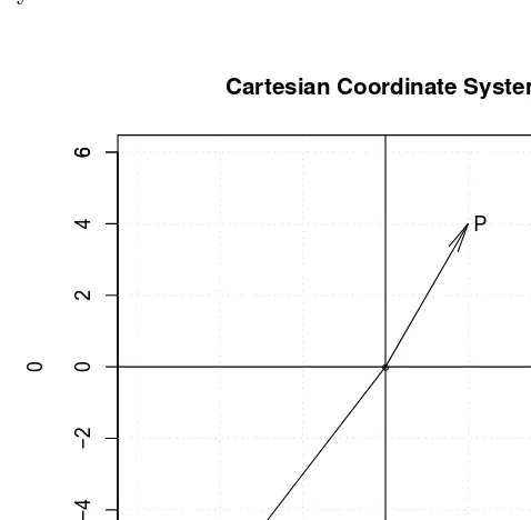
We begin with a simple plot of the Cartesian coordinate system using R. Recall from Sec. 1.6 that along each line of code, R ignores all text appearing after the # symbol. Section 1.5 item v described this. The snippet 2.2.1 uses the hash symbols to provide comments and remind ourselves and the reader what the nearby commands are doing. The reader should read the snippet comments and use the snippet as a template for using R graphics.
# R program snippet2.2.1plots coordinate system. #first plot the origin and set up limits of axes plot(0,0, xlim=c(-6,6), ylim=c(-6,6),
#now provide heading for the plot main="Cartesian Coordinate System") #plot command ended, Now Axes tick marks Axis(c(-6,6),at=c(-6,6),side=1)
Axis(c(-6,6),at=c(-6,6),side=2)
grid() #explicity display the grid
abline(h=0) #draw horizontal axis line at the origin
abline(v=0) #draw vertical line at the origin
# point P with x=2, y=4 as coordinates text(2.3,4,"P") #place text P on the graph
text(-4.3,-6,"Q")# at specified coordinates. Note that for #better visibility, horizontal coordinate is 0.3 units away. arrows(0,0,2,4, angle=10)#command to draw vector as arrows. arrows(0,0,-4,-6, angle=10)# with angle of the arrow tip
two-dimensional plane is obtained.
In a Euclidean space the ‘Real line’ is represented by all real numbers in the infinite range represented by the open interval: (−∞,∞).Parts of the real line falling within the limits of the graph are seen at the horizontal line (axis) passing through the values whenx= 0 andy= 0 (i.e., the origin at (0, 0) coordinate values). The figure represents an illustration of a two-dimensional Euclidian space split into four quadrants along four directions. Figure 2.1 also shows a grid representing the Cartesian coordinate system. We display two points P and Q in the North-East and South-West quadrants of the system.
●
−6 −4 −2 0 2 4 6
−6
−4
−2
0
2
4
6
Cartesian Coordinate System
0
0
−6 6
−6
6
P
Q
Fig. 2.1 The Cartesian coordinate system illustrated with point P(2,4) atx= 2, y= 4 as coordinates in the North-East quadrant and point Q(−4,−6) in the South-West quadrant.
Figure 2.1 also shows arrows representing vectors P = (2,4) and
axis andy units on the vertical axis.
More generally, thexaxis can be the real line in the infinite open interval mentioned above. Similarly, the y axis can also be the real line ℜ placed at 90o. Any point in this coordinate system formed by the two axes is
represented by an ‘ordered pair’ of numbers (x, y), where it is customary to state thexcoordinate value first. A two-dimensional space is represented by the Cartesian product denoted by the symbol (⊗) representing a set of ordered pairs of a set of xcoordinate values with a set ofy coordinate values:
ℜ ⊗ ℜ={(x, y) :x∈ ℜ, y∈ ℜ}=ℜ2. (2.2) Although the geometry might be difficult to represent on a piece of paper beyond two or three dimensions, nothing can stop us from imagining longer ordered values containing 3, 4 or any number nof coordinate axes. For example, (1,1,1,1) as an ordered set of 4 numbers can represent the unit point in a 4 dimensional space.
Thus we can think of n dimensional Euclidean space. Now define the Euclidean distance between point P with coordinates (p1, p2, . . . pn) and
pointQwith coordinates (q1, q2, . . . , qn) as:
d(P, Q) =√Σn
i=1(pi−qi)2. (2.3)
Writing our own functions is a very useful facility in R to reduce tedious repetitious tasks in a compact, efficient and accurate way. We have encoun-tered ‘myfunction’ in 1.6.1 for squaring one input and finding the sine of the second input. Here we illustrate a less trivial function. Section 5.7 has an R function with dozens of lines of code to compute answers to all types of payoff decision problems.
snippet 2.2.2 our function returns the Euclidean distance between the two input vectors as its output. The function is fully created in the first three lines of code of the snippet. The last three lines compute the distance for 1 to 3 dimensional vectors as inputs.
# R program snippet2.2.2is next.
Eudist = function(p,q) { #function begins here
ou1=(p-q)^2 #compute squared differences
return(sqrt(sum(ou1)))} #function ends here Eudist(1,6) #one-dimensional distance
Eudist(c(2,4),c(-4,-6)) #2 dimensional distance Eudist(c(2,3,4),c(2,8,16)) #3 dimensional distance
Recall the Figure 2.1 with arrows representing vectors P = (2,4) and
Q = (−4,−6). The snippet 2.2.2 finds the Euclidean distance between these two points to be 11.66190. The output of the above code snippet is given next.
> Eudist(1,6) #one-dimensional distance [1] 5
> Eudist(c(2,4),c(-4,-6)) #2 dimensional distance [1] 11.66190
> Eudist(c(2,3,4),c(2,8,16)) #3 dimensional distance [1] 13
Given two points P and Q defined above, their convex combination for the n-dimensional case is the set of points x∈ ℜn obtained for some
λ ∈ [0,1] so that x =λP + (1−λ)Q or more explicitly x =λp1+ (1−
λ)q1+. . . λpn+ (1−λ)qn.
2.2.1 Graphs for Simple Mathematical Functions and Equations
We have seen the plots of points similar to P and Q in Fig. 2.1 by using the ‘plot’ function of R. Now, we turn to plots for mathematical functions sometimes denoted as y = f(x), where the equality sign represents an explicit equation defining y from any set of values of x. The function of two variables may be stated implicitly as f(x, y) = 0. Some trigonometric functions (such astan(θ)) are used in this subsection for handling angles.
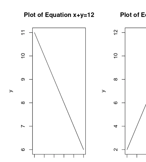
numbers. The correspondingy = 11,10,9,8,7,6.are implied by the equa-tion x+y = 12. The following R commands will produce the left panel of Fig. 2.2. The right panel of Fig. 2.2 represents the function y = 2x
produced by the code in the lower part of the following snippet.
# R program snippet2.2.1.1plots two lines.
par(mfrow=c(1,2))#plot format to have 1 row and 2 columns
x=1:6 #enter a sequence of numbers 1 to 6 as x
y=(12-1:6) #enter the y sequence from eq x+y=12 #plot command: main=main heading,
#typ="l" asks R to draw a line type plot
plot(x,y, main="Plot of Equation x+y=12", typ="l") x2=2*x
plot(x,x2, main="Plot of Equation y=2x", typ="l", ylab="y") #label y axis as y not x2
par(mfrow=c(1,1))# reset plot format to 1 row 1 column
The entire snippet(s) can be copied and pasted into R for implementation. Note from Fig. 2.2 that R automatically chooses the appropriate scaling for the vertical axis.
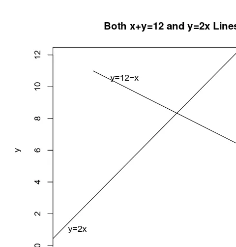
Angle between two straight lines:
If y = a1x+b1 and y = a2x+b2 are equations of two lines then
tanθ = (a2−a1)/(1 +a1a2) gives the angle through which the first line
must be rotated to make it parallel to the second line.
For the example of two lines plotted in Fig. 2.2 we havey= 12−x, b1=
12, a1=−1 andy = 2x, b2= 0, a2 = 2, respectively. Now tanθ= 3/(−1).
tan−1θ=−1.249046 radians or−71.56505 degrees computed by using the
R function ‘atan’ for inverse tangent or arc tangent with the command ‘atan(-3)*57.29578’. We can visualize the two curves together so that the angle between them can be visually seen. Hence, we use the following snippet.
# R program snippet2.2.1.2is next.
#R.snippet, assuming previous snippet is in memory plot(x,y, main="Both x+y=12 and y=2x Lines", ylim=c(0,12),xlim=c(0,7), typ="l")
1 2 3 4 5 6
6
7
8
9
10
11
Plot of Equation x+y=12
x
y
1 2 3 4 5 6
2
4
6
8
10
12
Plot of Equation y=2x
x
y
Fig. 2.2 Simple equation plots in R
text(2,10.5,"y=12-x")
The above snippet 2.2.1.2 shows that it takes a little work to get two lines on the same plot in R. We have to set up the plotting region carefully. Note that the second line is drawn by the function ‘abline’ rather than ‘plot.’ Another way to do the same (not seen in the snippet) is to use the function ‘curve(2*x,add=TRUE),’ where the argument ‘add=TRUE’ tells R to add a function to the existing plot using existing values on the horizontal axis. The snippet also shows how to insert text in the plot by specifying the coordinate points. A little trial and error is needed to get it to look right.
2.3 Solving Linear Equation by Finding Roots
0 1 2 3 4 5 6 7
0
2
4
6
8
10
12
Both x+y=12 and y=2x Lines
x
y
y=2x
y=12−x
Fig. 2.3 Two mathematical equations plotted together to visualize the angle between them.
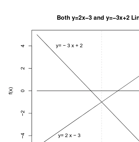
Solving it means that we want to find the correct number of values of x for which the equation holds true. Geometrically, y = 0 is a line and the number of solutions equals the number of timesf(x) touches or crosses the line.
Note that the angle between the two lines is only 45 degrees according to the formal computation. The tan(θ) = 1 is calculated in the snippet. The angle looks visually larger, since the range of the vertical axis [-4,4] is twice as wide as that of the horizontal axis [-1,3].
# R program snippet2.3.1is next. x=seq(-1,3,by=0.1)
y1=2*x-3
y2=-3*x+2; y3=rep(0,length(x))
text(0,-4, "y= 2 x - 3")
#above sets up scaling to include both lines lines(x,y2) #draws the second line
text(0, 4, "y= - 3 x + 2") lines(x, y3) #draws axis
grid(nx=2,ny=0, lwd=2) #wide vertical line at x=1 a1=2; a2=-3
tanTheta=(a2-a1)/(1+a1*a2)
theta=atan(tanTheta)*57.29578; theta
Now note that the solution of the equationf(x) = 2x−3 = 0 is atx= 3/2,
a positive value larger than 1 compared to the solution of the equation
f(x) =−3x+ 2 = 0 atx= 2/3, a value smaller than 1. Geometrically they are seen in Fig. 2.4 at two points where the liney= 0 meets the respective lines.
The equations need not be simply mathematical exercises, but can mean profound summaries of the macro economy. For example,y can represent the ‘real’ or inflation-adjusted interest rates andxcan represent the gross domestic product (GDP). Such an intersecting pair of equations is known as the ‘linear IS-LM model’ in macroeconomics. The line top left to bottom right is known a the ‘IS’ curve representing investments and savings behav-ior in response to interest rates. The line from bottom left to top right is called the ‘LM’ curve equating aggregate money demand with money supply. The point of intersection is known as the equilibrium solution of interest rate and GDP. Note that the intersection (equilibrium) occurs at a negative value of the interest rates (vertical axis). Of course, no bank can charge negative interest rate as a practical matter. Hence monetary policy cannot get the economy represented by Fig. 2.4 out of disequilibrium (re-cession). Only fiscal policy with deficit spending which will inject inflation can achieve an equilibrium. The point is that innocent looking equations can mean a great deal.
2.4 Polyroot Function in R
−1 0 1 2 3
−4
−2
0
2
4
Both y=2x−3 and y=−3x+2 Lines
x
f(x)
y= 2 x − 3 y= − 3 x + 2
Fig. 2.4 Solving two linear equationsf(x) = 2x−3 = 0 andf(x) =−3x+ 2 = 0.
The general formula for the quadratic equation is
f(x) =a x2+b x+c= 0, (2.4)
wherea, b, c are known constants. The roots of Eq. (2.4) are real numbers only if ρ = b2 −4a c ≥ 0, otherwise the roots are imaginary numbers.
Consider a simple example wherea = 1, b= −5, c= 6 having real roots. The general formula for two roots is:
x= −b±
√(b2−4a c)
2a . (2.5)
Substitutinga= 1, b=−5, c= 6 in Eq. (2.5) we find thatρ= 25−24 = 1, and the two roots arex1= [(5 + 1)/2] = 3, x2= [(5−1)/2] = 2. That is
the quadratic Eq. (2.4) can be factored as (x−3)(x−2).